Quantum noise memory effect of multiple scattered light

Abstract

We investigate frequency correlations in multiple scattered light that are present in the quantum fluctuations. The memory effect for quantum and classical noise is compared, and found to have markedly different frequency scaling, which was confirmed in a recent experiment. Furthermore, novel mesoscopic correlations are predicted that depend on the photon statistics of the incoming light.

Light propagating through a disordered distribution of strongly scattering particles induces an apparently random intensity pattern known as a volume speckle pattern. Despite the apparent randomness, such intensity speckle patterns can posses strong temporal and spatial correlations, giving rise to the so-called memory effect Feng88 . The memory effect manifests itself as strong correlation between different spatial directions or frequency components of the speckle pattern. After its demonstration in early experiments Freund88 ; Garcia91 , the memory effect has been employed as a sensitive technique of measuring the diffusion constant of light propagation Vellekoop05 . For extremely strong scattering, close to the transition to Anderson localization, classical intensity correlations can be strongly enhanced, which are referred to as mesoscopic correlations Scheffold98 ; Chabanov00 . Recently, it was shown that speckle correlations also exist when recording the fluctuations of light instead of merely the intensity Lodahl05-PRL . Furthermore, strong spatial quantum correlations were predicted depending on the quantum state of light incident on the medium Lodahl05-corr . In the present Letter we derive the noise correlation function, which was measured in Lodahl05-PRL , for an arbitrary quantum state of light. Our work demonstrates that the quantum fluctuations of a volume speckle pattern give rise to a strong memory effect that behaves different than classical fluctuations and also different than the classical memory effect for intensities.

We study the propagation of photons through a multiple scattering random medium. Using the quantum model for multiple scattering Beenakker98 , we discretize the system into $N$ different input modes and output modes. Let $\hat{n}_{\omega}^{ab}$ denote the photon number operator for light at the frequency $\omega$ propagating from input channel $a$ to output channel $b$. The fluctuations are quantified by the photon number variance $(\Delta n_{\omega}^{ab})^{2}=\left<({\hat{n}_{\omega}^{ab}})^{2}\right>-\left<{\hat{n}_{\omega}^{ab}}\right>^{2},$ where the quantum mechanical expectation value will be evaluated for different quantum states of light. Further details about this model are given in Lodahl05-corr . The quantum noise frequency correlation function for light propagating from input channel $a$ to output channel $b$ is defined by

$$C_{ab}^{N}(\Delta\omega)=\frac{\overline{(\Delta n_{\omega}^{ab})^{2}\times(\Delta n_{\omega+\Delta\omega}^{ab})^{2}}}{\overline{(\Delta n_{\omega}^{ab})^{2}}^{2}}-1.$$ (1)

This function measures the correlation between the fluctuations in a specific output direction for a frequency offset of $\Delta\omega$, and is the generalization of intensity correlation functions to the case of photon number fluctuations. The bars above the variances denote averaging over ensembles of disorder. We consider an arbitrary quantum state of light coupled through channel $a$ characterized by an averaged number of photons $\left<\hat{n}_{\omega}^{a}\right>$ and a Fano factor $F_{a}=(\Delta n_{\omega}^{a})^{2}/\left<\hat{n}_{\omega}^{a}\right>$. The photon number fluctuations of light transmitted to channel $b$ is given by Lodahl05-corr

$$\left[{(\Delta n_{\omega}^{ab})^{2}}\right]_{QN}=\left<\hat{n}_{\omega}^{a}\right>{T_{\omega}^{ab}}+\left<\hat{n}_{\omega}^{a}\right>(F_{a}-1){(T_{\omega}^{ab})^{2}},$$ (2)

where $T_{\omega}^{ab}$ is the intensity transmission coefficient from channel $a$ to channel $b$. Here the subscript QN refers to quantum noise of the relevant quantum state. In the situation where classical noise (CN) is dominating, which, e.g., is the case when modulating a laser beam, the variance of the fluctuations is proportional to the squared average number of photons Lodahl05-PRL

$$\left[{(\Delta n_{\omega}^{ab})^{2}}\right]_{CN}\propto\left<\hat{n}_{\omega}^{a}\right>^{2}{(T_{\omega}^{ab})^{2}}.$$ (3)

Consequently, the correlation functions for quantum and classical noise are given by

$$C_{ab}^{QN}(\Delta\omega) = \frac{\overline{T_{\omega}T_{\omega+\Delta\omega}}+(F_{a}-1)\left[\overline{T_{\omega}^{2}T_{\omega+\Delta\omega}}+\overline{T_{\omega}T_{\omega+\Delta\omega}^{2}}\right]+(F_{a}-1)^{2}\overline{T_{\omega}^{2}T_{\omega+\Delta\omega}^{2}}}{\overline{T_{\omega}}^{2}+2(F_{a}-1)\overline{T_{\omega}}\times\overline{T_{\omega}^{2}}+(F_{a}-1)^{2}\overline{T_{\omega}^{2}}^{2}}-1,$$ (4a)

$$C_{ab}^{CN}(\Delta\omega) = \frac{\overline{T_{\omega}^{2}T_{\omega+\Delta\omega}^{2}}}{\overline{T_{\omega}^{2}}^{2}}-1,$$ (4b)

where we have assumed $\left<\hat{n}_{\omega}\right>=\left<\hat{n}_{\omega+\Delta\omega}\right>$ corresponding to the situation where the input number of photons is kept constant when varying the optical frequency, which was the case in the experiment in Lodahl05-PRL . Note that we have skipped the indices $ab$ on the transmission coefficients in order to simplify notation.

In the lowest order approximation, the electric field transmission coefficient $t_{\omega}$ can be described by a circular Gaussian process, where $T_{\omega}=\left|t_{\omega}\right|^{2}$. For such Gaussian random variables, we have Goodman

$$\overline{t_{1}^{*}\ldots t_{k}^{*}t_{k+1}\ldots t_{2k}}=\sum_{\pi}\overline{t_{1}^{*}t_{p}}\times\overline{t_{2}^{*}t_{q}}\times\ldots\times\overline{t_{k}^{*}t_{r}},$$ (5)

where the summation is over all $k!$ permutations of the indices. Based on this theorem, we can evaluate the moments of $T_{\omega}$ that are relevant for Eqs. (4a) and (4b) :

$$\overline{T_{\omega}T_{\omega+\Delta\omega}} = \overline{T_{\omega}}^{2}+\left|\overline{t_{\omega}^{*}t_{\omega+\Delta\omega}}\right|^{2},$$ (6a)

$$\overline{T_{\omega}^{2}T_{\omega+\Delta\omega}} = \overline{T_{\omega}T_{\omega+\Delta\omega}^{2}}=2\overline{T_{\omega}}^{3}+4\overline{T_{\omega}}\left|\overline{t_{\omega}^{*}t_{\omega+\Delta\omega}}\right|^{2},$$ (6b)

$$\overline{T_{\omega}^{2}T_{\omega+\Delta\omega}^{2}} = 4\overline{T_{\omega}}^{4}+16\overline{T_{\omega}}^{2}\left|\overline{t_{\omega}^{*}t_{\omega+\Delta\omega}}\right|^{2}+4\left|\overline{t_{\omega}^{*}t_{\omega+\Delta\omega}}\right|^{4},$$

$$\overline{T_{\omega}^{n}} = n!\overline{T_{\omega}}^{n}$$ (6d)

First, for the quantum noise, let us restrict to the special case of shot noise (SN), which corresponds to $F_{a}=1$. Hence, the correlation functions in Eqs. (4a) and (4b) are given by

$$C_{ab}^{SN}(\Delta\omega) = \frac{\left|\overline{t_{\omega}^{*}t_{\omega+\Delta\omega}}\right|^{2}}{{\overline{T_{\omega}}}^{2}}\equiv f(\Delta\omega),$$ (7a)

$$C_{ab}^{CN}(\Delta\omega) = \frac{\left|\overline{t_{\omega}^{*}t_{\omega+\Delta\omega}}\right|^{4}+4\overline{T_{\omega}}^{2}\left|\overline{t_{\omega}^{*}t_{\omega+\Delta\omega}}\right|^{2}}{\overline{T_{\omega}}^{4}}$$ (7b)

$$\equiv f^{2}(\Delta\omega)+4f(\Delta\omega),$$

where

$$f(\Delta\omega)=\frac{\Delta\omega/\omega_{D}}{\cosh(\sqrt{\Delta\omega/\omega_{D}})-\cos(\sqrt{\Delta\omega/\omega_{D}})},$$ (8)

is the function that describes the frequency decay of the intensity correlations Berkovits94 with $\omega_{D}=D/2L^{2}$.

The correlation functions for shot noise and technical noise are plotted in Fig. 1 as a function of frequency offset $\Delta\omega$. We observe that the noise correlations are much stronger in the case of classical noise relative to shot noise, thus the correlation at $\Delta\omega=0$ is a factor $5$ higher. This pronounced difference was verified experimentally in Lodahl05-PRL . We note that the correlation function for shot noise is identical to what one would get if recording the intensity, the latter being independent of the actual quantum state. Notably, the quantum fluctuations provide an independent measure of frequency speckle correlations, and as will be seen in the following, the noise correlations depend strongly on the quantum state of light used in the experiment.

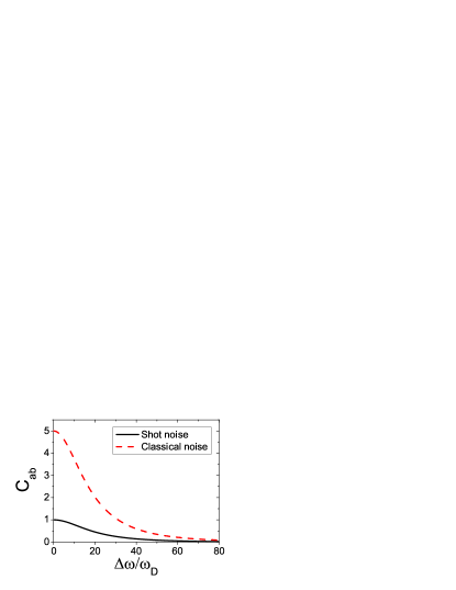
Figure 1: Noise correlation function for shot noise (full curve) and classical noise (dashed curve) as a function of frequency offset.

In the general case of an arbitrary quantum state characterized by the Fano factor $F_{a}$, the correlation function is given by Eq. (4a). This expression contains terms of various orders in $\overline{T_{\omega}}$, where in general $\overline{T_{\omega}}\ll 1,$ i.e. Eq. (4a) can be expanded in orders of the intensity transmission coefficient. In this expansion of the products of transmission coefficients also higher-order contributions must be included that originate from deviations from Gaussian statistics of the transmission coefficients. The lowest order contribution of such mesoscopic correlations provides a correction term in the product of two transmission coefficients deBoer02 ; deBoer_thesis

$$\overline{T_{\omega}T_{\omega+\Delta\omega}}=\overline{T_{\omega}}^{2}+\left|\overline{t_{\omega}^{*}t_{\omega+\Delta\omega}}\right|^{2}+\frac{3L^{2}}{2\ell^{2}}g(\Delta\omega)\overline{T_{\omega}}^{3},$$ (9)

where $L$ is the thickness of the random medium, $\ell$ is the transport mean free path, and we have defined the function

$$g(\Delta\omega)=\frac{\omega_{D}}{\Delta\omega}\times\frac{\sinh(\sqrt{\Delta\omega/\omega_{D}})-\sin(\sqrt{\Delta\omega/\omega_{D}})}{\cosh(\sqrt{\Delta\omega/\omega_{D}})-\cos(\sqrt{\Delta\omega/\omega_{D}})}.$$ (10)

Expanding Eq. (4a) to first order leads to

$$C_{ab}^{QN}(\Delta\omega)\approx C_{ab}^{I}(\Delta\omega)+C_{ab}^{II}(\Delta\omega),$$ (11)

where

$$C_{ab}^{I}(\Delta\omega) = f(\Delta\omega),$$ (12a)

$$C_{ab}^{II}(\Delta\omega) = \frac{3L^{2}}{2\ell^{2}}g(\Delta\omega)\overline{T_{\omega}}+4(F_{a}-1)f(\Delta\omega)\overline{T_{\omega}}.$$

The dominating term in the expansion $(C_{ab}^{I})$ is simply equal to the contribution obtained with shot noise. Deviations from shot noise behavior is observed when using quantum states of light different from the coherent state, i.e. $F_{a}\neq 1,$ which gives rise to the second term in Eq. (LABEL:Cab-2order). The quantum correction competes with classical mesoscopic correlations (first term in Eq. (LABEL:Cab-2order)), which is in contrast to the dominating quantum corrections found in the fluctuations of the total transmission and reflection Lodahl05-corr .

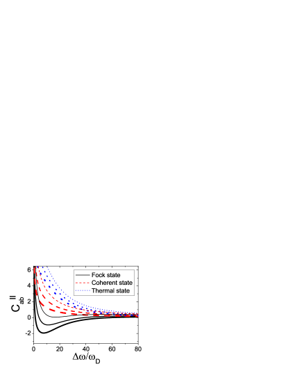
Figure 2: Second-order correlation function $C_{ab}^{II}$ normalized to $\overline{T_{\omega}}$ as a function of frequency offset for three different quantum states of light: Fock state $F_{a}=0$ (solid line), coherent state $F_{a}=1$ (dashed line) and thermal state $F_{a}=2$ (dotted line). The ratios of mean free path to the sample thickness are $\ell/L=1/3$ (bold lines), $\ell/L=1/4$ (medium lines), and $\ell/L=1/5$ (thin lines).

In Fig. 2, we plot the second-order noise correlation function $C_{ab}^{II}(\Delta\omega)$ for three different quantum states of light, corresponding to $F_{a}=0$, $F_{a}=1$, and $F_{a}=2.$ These Fano factors can be achieved with single-mode Fock states, coherent states and thermal states, respectively Lodahl05-corr . Figure 2 also indicates the correlation function for different ratios $\ell/L$, where $\ell/L\ll 1$ for optical media where multiple scattering dominates. The classical mesoscopic correlations, which also can be extracted from intensity measurements, are obtained for $F_{a}=1.$ In the limit $\Delta\omega/\omega_{D}\rightarrow 0,$ the classical correlation function diverges, which is a consequence of the plane-wave approximation and is suppressed when including finite-width beams deBoer02 . This sensitivity to the width of the beam only plays an important role for the correlations at $\Delta\omega/\omega_{D}\sim 1.$ We observe from Fig. 2 that either positive or negative quantum noise correlations are obtained using either super-Poissonian ($F_{a}>1$) or sub-Poissonian photons ($F_{a}<1$), respectively. Consequently, the fluctuations are found to possess novel correlations depending on the quantum state of light, which is markedly different from intensity correlations that are independent of the quantum state.

A novel noise correlation function for multiple scattered light was introduced and evaluated for both classical noise and for arbitrary single-mode quantum states. Pronounced different correlations were found when comparing classical noise to quantum noise. Including higher-order correction terms in an expansion in the transmission coefficient, quantum corrections to the noise correlation function were predicted that have no analogy in classical intensity measurements.

I would like to thank Ad Lagendijk for fruitful discussions and encouragement. The work is supported by the Danish Research Agency.

References

• (1) S. Feng, C. Kane, P.A. Lee, and A.D. Stone, Phys. Rev. Lett. 61, 834 (1988).
• (2) I. Freund, M. Rosenbluh, and S. Feng, Phys. Rev. Lett. 61, 2328 (1988).
• (3) N. Garzia and A.Z. Genack, Opt. Lett. 16, 1132 (1991).
• (4) I. Vellekoop, P. Lodahl, and A. Lagendijk, Phys. Rev. E 71, 056604 (2005).
• (5) F. Scheffold and G. Maret, Phys. Rev. Lett. 81, 5800 (1998).
• (6) A.A. Chabanov, M. Stoytchev, and A.Z. Genack, Nature 404, 850 (2000).
• (7) P. Lodahl and A. Lagendijk, Phys. Rev. Lett. 94, 153905 (2005).
• (8) P. Lodahl, A.P. Mosk, and A. Lagendijk, http://arxiv.org/abs/quant-ph/0502033 (2005).
• (9) C.W.J. Beenakker, Phys. Rev. Lett. 81, 1829 (1998).
• (10) J.W. Goodman, Statistical Optics (John Wiley & Sons, New York, 1985).
• (11) R. Berkovits and S. Feng, Phys. Rep. 238, 135 (1994).
• (12) J.F. de Boer, M.P. van Albada, and A. Lagendijk, Phys. Rev. B 45, 658 (1992).
• (13) J.F. de Boer, Optical fluctuations on the transmission and reflection of mesoscopic systems, (Ph.D. Thesis, University of Amsterdam, 1995), available on: www.tn.utwente.nl/cops/pdf/theses/deboer.pdf.