Entanglement, Purity, and Information Entropies
in Continuous Variable Systems

Abstract

Quantum entanglement of pure states of a bipartite system is defined as the amount of local or marginal (i.e. referring to the subsystems) entropy. For mixed states this identification vanishes, since the global loss of information about the state makes it impossible to distinguish between quantum and classical correlations. Here we show how the joint knowledge of the global and marginal degrees of information of a quantum state, quantified by the purities or in general by information entropies, provides an accurate characterization of its entanglement. In particular, for Gaussian states of continuous variable systems, we classify the entanglement of two–mode states according to their degree of total and partial mixedness, comparing the different roles played by the purity and the generalized $p-$entropies in quantifying the mixedness and bounding the entanglement. We prove the existence of strict upper and lower bounds on the entanglement and the existence of extremally (maximally and minimally) entangled states at fixed global and marginal degrees of information. This results allow for a powerful, operative method to measure mixed-state entanglement without the full tomographic reconstruction of the state. Finally, we briefly discuss the ongoing extension of our analysis to the quantification of multipartite entanglement in highly symmetric Gaussian states of arbitrary $1\times N$-mode partitions.

1. Introduction

According to Erwin Schrödinger, quantum entanglement is not “one but rather the characteristic trait of quantum mechanics, the one that enforces its entire departure from classical lines of thought” [1]. Entanglement has been widely recognized as a fundamental aspect of quantum theory, stemming directly from the superposition principle and quantum non factorizability. Remarkably, it is now also acknowledged as a fundamental physical resource, much on the same status as energy and entropy, and as a key factor in the realization of information processes otherwise impossible to implement on classical systems. Thus the degree of entanglement and information are the crucial features of a quantum state from the point of view of Quantum Information Theory [2]. Indeed, the search for proper mathematical frameworks to quantify such features in generic (mixed) quantum states cannot be yet considered accomplished. In view of such considerations, it is clear that the full understanding of the relationships between the quantum correlations contained in a multipartite state and the global and local (i.e. referring to the reduced states of the subsystems) degrees of information of the state, is of critical importance. In particular, it would represent a relevant step towards the clarification of the nature of quantum correlations and, possibly, of the distinction between quantum and classical correlations of mixed states [3]. The main question we want to address in this work is:

What can we say about the quantum correlations existing between the subsystems of a quantum multipartite system in a mixed state, if we know the degrees of information carried by the global and the reduced states?

We can anticipate that the answer will be “almost everything” in the context of Gaussian states of continuous variable systems. To this aim, we will start by briefly reviewing in Sec. 2. the properties of Gaussian states in infinite–dimensional Hilbert spaces, and the concepts of information and entanglement. In Sec. 3. we will show, step by step, how the entanglement of two–mode Gaussian states can be accurately characterized by the knowledge of global and marginal degrees of information, quantified by the purities, or by the generalized entropies of the global state and of the reduced states of the subsystems. In Sec. 4. we will give a brief sketch of the generalization of our methods to the quantification of multipartite entanglement in multimode Gaussian states under symmetry. Finally, in Sec. 5. we will summarize our results and discuss future perspectives.

2. Gaussian states: general properties

We consider a continuous variable (CV) system consisting of $N$ canonical bosonic modes, associated to an infinite-dimensional Hilbert space and described by the vector $\hat{X}=\{\hat{x}_{1},\hat{p}_{1},\ldots,\hat{x}_{N},\hat{p}_{N}\}$ of the field quadrature (“position” and “momentum”) operators. The quadrature phase operators are connected to the annihilation $\hat{a}_{i}$ and creation $\hat{a}^{{\dagger}}_{i}$ operators of each mode, by the relations $\hat{x}_{i}=(\hat{a}_{i}+\hat{a}^{{\dagger}}_{i})$ and $\hat{p}_{i}=(\hat{a}_{i}-\hat{a}^{{\dagger}}_{i})/i$. The canonical commutation relations for the $\hat{X}_{i}$’s can be expressed in matrix form: $[\hat{X}_{i},\hat{X}_{j}]=2i\Omega_{ij}$, with the symplectic form $\Omega=\oplus_{i=1}^{n}\omega$ and $\omega=\delta_{ij-1}-\delta_{ij+1},\,i,j=1,2$.

Quantum states of paramount importance in CV systems are the so-called Gaussian states, i.e. states with Gaussian characteristic functions and quasi–probability distributions [4]. The interest in this special class of states (important examples are vacua, coherent, squeezed and thermal states of the electromagnetic field) stems from the feasibility to produce and control them with linear optics, and from the increasing number of efficient proposals and successful experimental implementations of CV quantum information and communication processes involving multimode Gaussian states (see [5] for a recent review). By definition, a Gaussian state is completely characterized by first and second moments of the canonical operators. When addressing physical properties invariant under local unitary transformations, such as the mixedness and the entanglement, one can neglect first moments and completely characterize Gaussian states by the $2N\times 2N$ real covariance matrix (CM) $\boldsymbol{\sigma}$, whose entries are $\sigma_{ij}=1/2\langle\{\hat{X}_{i},\hat{X}_{j}\}\rangle-\langle\hat{X}_{i}\rangle\langle\hat{X}_{j}\rangle$. Throughout the paper, $\boldsymbol{\sigma}$ will be used indifferently to indicate the CM of a Gaussian state or the state itself. A real, symmetric matrix $\boldsymbol{\sigma}$ must fulfill the Robertson-Schrödinger uncertainty relation [6]

$$\boldsymbol{\sigma}+i\Omega\geq 0\,,$$ (1)

to be a bona fide CM of a physical state. Symplectic operations (i.e. belonging to the group $Sp_{(2N,\mathbbm{R})}=\{S\in SL(2N,\mathbbm{R})\,:\,S^{T}\Omega S=\Omega\}$) acting by congruence on CMs in phase space, amount to unitary operations on density matrices in Hilbert space. In phase space, any $N$-mode Gaussian state can be transformed by symplectic operations in its Williamson diagonal form $\boldsymbol{\nu}$ [7], such that $\boldsymbol{\sigma}=S^{T}\boldsymbol{\nu}S$, with $\boldsymbol{\nu}=\,{\rm diag}\,\{\nu_{1},\nu_{1},\ldots\nu_{N},\nu_{N}\}$. The set $\Sigma=\{\nu_{i}\}$ constitutes the symplectic spectrum of $\boldsymbol{\sigma}$ and its elements must fulfill the conditions $\nu_{i}\geq 1$, following from Eq. (1) and ensuring positivity of the density matrix associated to $\boldsymbol{\sigma}$. We remark that the full saturation of the uncertainty principle can only be achieved by pure $N$-mode Gaussian states, for which $\nu_{i}=1\,\,\forall i=1,\ldots,N$. Instead, mixed states such that $\nu_{i\leq k}=1$ and $\nu_{i>k}>1$, with $1\leq k\leq N$, only partially saturate the uncertainty principle, with partial saturation becoming weaker with decreasing $k$. The symplectic eigenvalues $\nu_{i}$ can be computed as the orthogonal eigenvalues of the matrix $|i\Omega\boldsymbol{\sigma}|$, so they are determined by $N$ symplectic invariants associated to the characteristic polynomial of such a matrix. Two global invariants which will be useful are the determinant $\,{\rm Det}\,\boldsymbol{\sigma}=\prod_{i}\nu_{i}^{2}$ and the seralian [8] $\Delta=\sum_{i}\nu_{i}^{2}$, which is the sum of the determinants of all the $2\times 2$ submatrices of $\boldsymbol{\sigma}$ related to each mode.

The degree of information about the preparation of a quantum state $\varrho$ can be characterized by its purity $\mu\equiv\,{\rm Tr}\,\varrho^{2}$. For a Gaussian state with CM $\boldsymbol{\sigma}$ one has simply $\mu=1/\sqrt{\,{\rm Det}\,\boldsymbol{\sigma}}$ [9]. In general, the mixedness, or lack of information about the preparation of the state, can be quantified by generalized entropic measures, such as the Bastiaans–Tsallis entropies [10, 11] $S_{p}\equiv(1-\,{\rm Tr}\,\varrho^{p})/(p-1)$, which reduce to the linear entropy $S_{L}=1-\mu$ for $p=2$, and the Rényi entropies [12] $S_{p}^{R}\equiv(\log\,{\rm Tr}\,\varrho^{p})/(1-p)$. Both entropic families are parametrized by $p>1$ and it can be easily shown that $\lim_{p\rightarrow 1+}S_{p}=\lim_{p\rightarrow 1+}S_{p}^{R}=-\,{\rm Tr}\,(\varrho\log\varrho)\equiv S_{V}$, so that also the Shannon-von Neumann entropy $S_{V}$ can be defined in terms of generalized entropies. The quantity $S_{V}$ is additive on tensor product states and provides a further convenient measure of mixedness of the quantum state $\varrho$.

As for the entanglement, we recall that positivity of the CM’s partial transpose (PPT) [13] is a necessary and sufficient condition of separability for $(N+1)$-mode Gaussian states with respect to $1\times N$-mode partitions [14]. In phase space, partial transposition amounts to a mirror reflection of one quadrature associated to the single-mode partition. If $\{\tilde{\nu}_{i}\}$ is the symplectic spectrum of the partially transposed CM $\tilde{\boldsymbol{\sigma}}$, then a $(N+1)$-mode Gaussian state with CM $\boldsymbol{\sigma}$ is separable if and only if $\tilde{\nu}_{i}\geq 1$ $\forall\,i$. A convenient measure of CV entanglement is the logarithmic negativity [15] $E_{{\cal N}}\equiv\log\|\tilde{\varrho}\|_{1}$, $\|\cdot\|_{1}$ denoting the trace norm, which constitutes an upper bound to the distillable entanglement of the quantum state $\varrho$. It can be readily computed in terms of the symplectic spectrum $\tilde{\nu}_{i}$ of $\tilde{\boldsymbol{\sigma}}$, yielding [16]

$$E_{{\cal N}}=\left\{\begin{array}[]{cc}0,&\tilde{\nu}_{i}\geq 1\;\forall\,i\,;\\ -\sum_{i:\tilde{\nu}_{i}<1}\log\tilde{\nu}_{i}\,,&\hbox{else .}\\ \end{array}\right.$$ (2)

The logarithmic negativity quantifies the extent to which the PPT condition $\tilde{\nu}_{i}\geq 1$ is violated.

3. Characterizing two–mode entanglement by information measures

3.1. Parametrization of Gaussian states with symplectic invariants

Two–mode Gaussian states represent the prototypical quantum states of CV systems. Their CM can be written is the following block form

$$\boldsymbol{\sigma}\equiv\left(\begin{array}[]{cc}\boldsymbol{\alpha}&\boldsymbol{\gamma}\\ \boldsymbol{\gamma}^{T}&\boldsymbol{\beta}\end{array}\right)\,,$$ (3)

where the three $2\times 2$ matrices $\boldsymbol{\alpha}$, $\boldsymbol{\beta}$, $\boldsymbol{\gamma}$ are, respectively, the CMs of the two reduced modes and the correlation matrix between them. It is well known that for any two–mode CM $\boldsymbol{\sigma}$ there exists a local symplectic operation $S_{l}=S_{1}\oplus S_{2}$ which takes $\boldsymbol{\sigma}$ to the so called standard form $\boldsymbol{\sigma}_{sf}$ [17]

$$S_{l}^{T}\boldsymbol{\sigma}S_{l}=\boldsymbol{\sigma}_{sf}\equiv\left(\begin{array}[]{cccc}a&0&c_{+}&0\\ 0&a&0&c_{-}\\ c_{+}&0&b&0\\ 0&c_{-}&0&b\end{array}\right)\;.$$ (4)

States whose standard form fulfills $a=b$ are said to be symmetric. Let us recall that any pure state is symmetric and fulfills $c_{+}=-c_{-}=\sqrt{a^{2}-1}$. The uncertainty principle Ineq. (1) can be recast as a constraint on the $Sp_{(4,{\mathbb{R}})}$ invariants ${\rm Det}\boldsymbol{\sigma}$ and $\Delta(\boldsymbol{\sigma})={\rm Det}\boldsymbol{\alpha}+\,{\rm Det}\boldsymbol{\beta}+2\,{\rm Det}\boldsymbol{\gamma}$, yielding $\Delta(\boldsymbol{\sigma})\leq 1+\,{\rm Det}\boldsymbol{\sigma}$. The symplectic eigenvalues of a two–mode Gaussian state will be named $\nu_{-}$ and $\nu_{+}$, with $\nu_{-}\leq\nu_{+}$ in general. A simple expression for the $\nu_{\mp}$ can be found in terms of the two $Sp_{(4,\mathbb{R})}$ invariants [8]

$$2{\nu}_{\mp}^{2}=\Delta(\boldsymbol{\sigma})\mp\sqrt{\Delta(\boldsymbol{\sigma})^{2}-4\,{\rm Det}\,\boldsymbol{\sigma}}\,.$$ (5)

The standard form covariances $a$, $b$, $c_{+}$, and $c_{-}$ can be determined in terms of the two local symplectic invariants

$$\mu_{1}=({\rm Det}\,\boldsymbol{\alpha})^{-1/2}=1/a\,,\quad\mu_{2}=({\rm Det}\,\boldsymbol{\beta})^{-1/2}=1/b\,,$$ (6)

which are the marginal purities of the reduced single–mode states, and of the two global symplectic invariants

$$\mu=({\rm Det}\,\boldsymbol{\sigma})^{-1/2}=[(ab-c_{+}^{2})(ab-c_{-}^{2})]^{-1/2}\,,\quad\Delta=a^{2}+b^{2}+2c_{+}c_{-}\,,$$ (7)

which are the global purity and the seralian, respectively. Eqs. (6-7) can be inverted to provide the following physical parametrization of two–mode states in terms of the four independent parameters $\mu_{1},\,\mu_{2},\,\mu$, and $\Delta$ [18]:

$$a\,\,=\,\,\frac{1}{\mu_{1}}\,,\quad b = \frac{1}{\mu_{2}}\,,\quad c_{\pm}\,\,=\,\,\frac{\sqrt{\mu_{1}\mu_{2}}}{4}\,\big{(}\epsilon_{-}\pm\epsilon_{+}\big{)}\,,$$ (8)

$${\rm with}\quad\epsilon_{\mp} \equiv \sqrt{\left[\Delta-\frac{(\mu_{1}\mp\mu_{2})^{2}}{\mu_{1}^{2}\mu_{2}^{2}}\right]^{2}-\frac{4}{\mu^{2}}}\,.$$

The uncertainty principle and the existence of the radicals appearing in Eq. (8) impose the following constraints on the four invariants in order to describe a physical state

$$0 \leq \mu_{1,2}\,\,\leq\,\,1\,,$$ (9)

$$\mu_{1}\mu_{2} \leq \mu\,\,\leq\,\,\frac{\mu_{1}\mu_{2}}{\mu_{1}\mu_{2}+\left|\mu_{1}-\mu_{2}\right|}\,,$$ (10)

$$\frac{2}{\mu}+\frac{(\mu_{1}-\mu_{2})^{2}}{\mu_{1}^{2}\mu_{2}^{2}} \leq \Delta\,\,\leq\,\,1+\frac{1}{\mu^{2}}\,.$$ (11)

The physical meaning of these constraints, and the role of the extremal states (i.e. states whose invariants saturate the upper or lower bounds of Eqs. (10-11)) in relation to the entanglement, will be carefully investigated in the next subsections.

In terms of symplectic invariants, partial transposition corresponds to flipping the sign of ${\rm Det}\,\boldsymbol{\gamma}$, so that $\Delta$ turns into $\tilde{\Delta}=\Delta-4\,{\rm Det}\,\boldsymbol{\gamma}=-\Delta+2/\mu_{1}^{2}+2/\mu_{2}^{2}$. The symplectic eigenvalues of the CM $\boldsymbol{\sigma}$ and of its partial transpose $\tilde{\boldsymbol{\sigma}}$ are promptly determined in terms of symplectic invariants

$$2\nu_{\mp}^{2}=\Delta\mp\sqrt{\Delta^{2}-{\frac{4}{\mu^{2}}}}\,,\quad 2\tilde{\nu}_{\mp}^{2}=\tilde{\Delta}\mp\sqrt{\tilde{\Delta}^{2}-{\frac{4}{\mu^{2}}}}\,.$$ (12)

The PPT criterion yields a state $\boldsymbol{\sigma}$ separable if and only if $\tilde{\nu}_{-}\geq 1$. A bona fide measure of entanglement for two–mode Gaussian states should thus be a monotonically decreasing function of $\tilde{\nu}_{-}$ [19], quantifying the violation of the previous inequality. A computable entanglement monotone for generic two-mode Gaussian states is provided by the logarithmic negativity Eq. (2)

$$E_{{\cal N}}=\max\{0,-\log\,\tilde{\nu}_{-}\}\,.$$ (13)

In the special instance of symmetric Gaussian states, the entanglement of formation [20] is also computable [21] but, being again a decreasing function of $\tilde{\nu}_{-}$, it provides the same characterization of entanglement and is thus fully equivalent to the logarithmic negativity in this subcase.

3.2. Entanglement vs Information (I) – Maximal entanglement at fixed global purity

The first step towards giving an answer to our original question is to investigate the properties of extremally entangled states at a given degree of global information. Let us mention that, for two–qubit systems, the existence of maximally entangled states at fixed mixedness (MEMS) was first found numerically by Ishizaka and Hiroshima [22]. The discovery of such states spurred several theoretical works [23], aimed at exploring the relations between different measures of entanglement and mixedness [24] (strictly related to the questions of the ordering of these different measures [25], and to the volume of the set of mixed entangled states [26]).

Unfortunately, it is easy to show that a similar analysis in the CV scenario is meaningless. Indeed, for any fixed, finite global purity $\mu$ there exist infinitely many Gaussian states which are infinitely entangled. As an example, we can consider the class of (nonsymmetric) two–mode squeezed thermal states. Let $S_{r}=\exp(\frac{1}{2}ra_{1}a_{2}-\frac{1}{2}ra_{1}^{{\dagger}}a_{2}^{{\dagger}})$ be the two mode squeezing operator with real squeezing parameter $r\geq 0$, and let $\varrho^{{}_{\otimes}}_{\nu_{i}}$ be a tensor product of thermal states with CM ${\boldsymbol{\nu}}_{\nu_{\mp}}={\mathbbm{1}}_{2}\nu_{-}\oplus{\mathbbm{1}}_{2}\nu_{+}$, where $\nu_{\mp}$ is, as usual, the symplectic spectrum of the state. Then, a nonsymmetric two-mode squeezed thermal state $\xi_{\nu_{i},r}$ is defined as ${\xi}_{\nu_{i},r}=S_{r}\varrho^{{}_{\otimes}}_{\nu_{i}}S_{r}^{{\dagger}}$, corresponding to a standard form with

$$a = {\nu_{-}}\cosh^{2}r+{\nu_{+}}\sinh^{2}r\;,\quad b\,\,=\,\,{\nu_{-}}\sinh^{2}r+{\nu_{+}}\cosh^{2}r\;,$$ (14)

$$c_{\pm} = \pm\frac{\nu_{-}+\nu_{+}}{2}\sinh 2r\;.$$

For simplicity we can consider the symmetric instance ($\nu_{-}=\nu_{+}=1/\sqrt{\mu}$) and compute the logarithmic negativity Eq. (13), which takes the expression $E_{\cal N}(r,\mu)=-(1/2)\log[{\rm e}^{-4r}/\mu]$. Notice how the completely mixed state ($\mu\rightarrow 0$) is always separable while, for any $\mu>0$, we can freely increase the squeezing $r$ to obtain Gaussian states with arbitrarily large entanglement. For fixed squeezing, as naturally expected, the entanglement decreases with decreasing degree of purity of the state, analogously to what happens in discrete–variable MEMS [24].

3.3. Entanglement vs Information (II) – Maximal entanglement at fixed local purities

The next step in the analysis is the unveiling of the relation between the entanglement of a Gaussian state of CV systems and the degrees of information related to the subsystems. Maximally entangled states for given marginal mixednesses (MEMMS) have been recently introduced and analyzed in detail in the context of qubit systems by Adesso et al. [27]. The MEMMS provide a suitable generalization of pure states, in which the entanglement is completely quantified by the marginal degrees of mixedness.

For two–mode Gaussian states, it follows from the expression Eq. (12) of $\tilde{\nu}_{-}$ that, for fixed marginal purities $\mu_{1,2}$ and seralian $\Delta$, the logarithmic negativity is strictly increasing with increasing $\mu$. By imposing the saturation of the upper bound of Eq. (10), $\mu=\mu^{\max}(\mu_{1,2})\equiv(\mu_{1}\mu_{2})/(\mu_{1}\mu_{2}+\left|\mu_{1}-\mu_{2}\right|)$, we determine the most pure states for fixed marginals; moreover, choosing $\mu=\mu^{\max}(\mu_{1,2})$ immediately implies that the upper and the lower bounds on $\Delta$ of Eq. (11) coincide and $\Delta$ is uniquely determined in terms of $\mu_{1,2}$. This means that the two–mode states with maximal purity for fixed marginals are indeed the Gaussian maximally entangled states for fixed marginal mixednesses (GMEMMS). They can be seen as the CV analogues of the MEMMS.

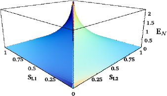
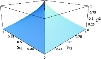
Fig. 1: Plot of the maximal entanglement achievable by quantum systems with given marginal linear entropies: (a) logarithmic negativity of continuous variable GMEMMS, which saturate the upper bound of inequality (10); (b) tangle of two–qubit MEMMS, introduced in Ref. [27].

In Fig. 1 the logarithmic negativity of GMEMMS is plotted (a) as a function of the marginal linear entropies $S_{L{1,2}}\equiv 1-\mu_{1,2}$, in comparison (b) with the behaviour of the tangle (an entanglement monotone equivalent to the entanglement of formation for two qubits [28]) as a function of $S_{L{1,2}}$ for discrete variable MEMMS. Notice, as a common feature, how the maximal entanglement achievable by quantum mixed states rapidly increases with increasing marginal mixednesses (like in the pure–state instance) and decreases with increasing difference of the marginals. This is natural, because the presence of quantum correlations between the subsystems implies that they should possess similar amounts of quantum information. Let us finally mention that the “minimally” entangled states for fixed marginals, which saturate the lower bound of Eq. (10) ($\mu=\mu_{1}\mu_{2}$), are just the tensor product states, i.e. states without any (quantum or classical) correlations between the subsystems.

3.4. Entanglement vs Information (III) – Extremal entanglement at fixed global and local purities

What we have shown so far, by simple analytical bounds, is a general trend of increasing entanglement with increasing global purity, and with decreasing marginal purities and difference between them. We now wish to exploit the joint information about global and marginal degrees of purity to achieve a significative characterization of entanglement, both qualitatively and quantitatively. Let us first investigate the role played by the seralian $\Delta$ in the characterization of the properties of Gaussian states. To this aim, we analyse the dependence of the eigenvalue $\tilde{\nu}_{-}$ on $\Delta$, for fixed $\mu_{1,2}$ and $\mu$:

$$\left.\frac{\partial\ \tilde{\nu}^{2}_{-}}{\partial\ \Delta}\right|_{\mu_{1},\,\mu_{2},\,\mu}\,=\;\frac{1}{2}\left(\frac{\tilde{\Delta}}{\sqrt{\tilde{\Delta}^{2}-{\frac{1}{4\mu^{2}}}}}-1\right)\,>0\,.$$ (15)

The smallest symplectic eigenvalue of the partially transposed state is strictly monotone in $\Delta$. Therefore the entanglement of a generic Gaussian state $\boldsymbol{\sigma}$ with given global purity $\mu$ and marginal purities $\mu_{1,2}$, strictly increases with decreasing $\Delta$. The seralian $\Delta$ is thus endowed with a direct physical interpretation: at given global and marginal purities, it determines the amount of entanglement of the state. Moreover, due to inequality (11), $\Delta$ is constrained both by lower and upper bounds; therefore, not only maximally but also minimally entangled Gaussian states exist. This fact admirably elucidates the relation between quantum correlations and information in two–mode Gaussian states: the entanglement of such states is tightly bound by the amount of global and marginal purities, with only one remaining degree of freedom related to the invariant $\Delta$ [29].

We now aim to characterize extremally (maximally and minimally) entangled Gaussian states for fixed global and marginal purities. Let us first consider the states saturating the lower bound in Eq. (11), which entails maximal entanglement and defines the class of Gaussian most entangled states for fixed global and local purities (GMEMS). It is easily seen that such states belong to the class of asymmetric two–mode squeezed thermal states Eq. (14), with squeezing parameter and symplectic spectrum

$$\tanh 2r = 2(\mu_{1}\mu_{2}-\mu_{1}^{2}\mu_{2}^{2}/\mu)^{1/2}/(\mu_{1}+\mu_{2})\,,$$ (16)

$$\nu_{\mp}^{2} = \frac{1}{\mu}+\frac{(\mu_{1}-\mu_{2})^{2}}{2\mu_{1}^{2}\mu_{2}^{2}}\mp\frac{|\mu_{1}-\mu_{2}|}{2\mu_{1}\mu_{2}}\sqrt{\frac{(\mu_{1}-\mu_{2})^{2}}{\mu_{1}^{2}\mu_{2}^{2}}+\frac{4}{\mu}}\,.$$ (17)

Nonsymmetric two–mode thermal squeezed states turn out to be separable in the range

$$\mu\leq\frac{\mu_{1}\mu_{2}}{\mu_{1}+\mu_{2}-\mu_{1}\mu_{2}}\,.$$ (18)

As a consequence, all Gaussian states whose purities fall in the separable region defined by inequality (18) are not entangled.

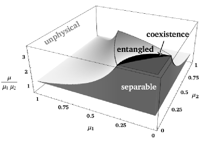
Degrees of Purity	Regions
$\mu<\mu_{1}\mu_{2}$	unphysical
$\mu_{1}\mu_{2}\;\leq\;\mu\;\leq\;\frac{\mu_{1}\mu_{2}}{\mu_{1}+\mu_{2}-\mu_{1}\mu_{2}}$	separable
$\frac{\mu_{1}\mu_{2}}{\mu_{1}+\mu_{2}-\mu_{1}\mu_{2}}<\mu\leq\frac{\mu_{1}\mu_{2}}{\sqrt{\mu_{1}^{2}+\mu_{2}^{2}-\mu_{1}^{2}\mu_{2}^{2}}}$	coexistence
$\frac{\mu_{1}\mu_{2}}{\sqrt{\mu_{1}^{2}+\mu_{2}^{2}-\mu_{1}^{2}\mu_{2}^{2}}}<\mu\leq\frac{\mu_{1}\mu_{2}}{\mu_{1}\mu_{2}+\left|\mu_{1}-\mu_{2}\right|}$	entangled
$\mu>\frac{\mu_{1}\mu_{2}}{\mu_{1}\mu_{2}+\left|\mu_{1}-\mu_{2}\right|}$	unphysical

Table I

Fig. 2: Summary of entanglement properties of two–mode Gaussian states in the space of marginal purities $\mu_{1,2}$ ($x$- and $y$-axes) and global purity $\mu$ (on the $z$-axis we plot the ratio $\mu/\mu_{1}\mu_{2}$ to gain a better graphical distinction between the various regions). In this space, all physical states lay between the horizontal plane $z=1$ representing product states, and the upper limiting surface representing GMEMMS (see Fig. 1a). Separable and entangled states are well distinguished except for a narrow coexistence region (depicted in black). The first ones fill the region depicted in dark grey, while in the area containing only entangled states the average logarithmic negativity Eq. (23) grows from white to medium grey. The mathematical relations defining the boundaries between all these regions are collected in Table I. The 3D envelope is cut at $z=3.5$.

We next consider the states that saturate the upper bound in Eq. (11). They determine the class of Gaussian least entangled states for given global and local purities (GLEMS) and, outside the separable region (where every Gaussian state can be considered a GLEMS having zero entanglement), they fulfill $\Delta=1+1/{\mu}^{2}$. This relation implies that the symplectic spectrum of these states takes the form $\nu_{-}=1$, $\nu_{+}=1/\mu$. We thus find that GLEMS are mixed Gaussian states of partial minimum uncertainty, so in some sense they are the most classical ones and this is consistent with their property of having minimal entanglement. According to the PPT criterion, GLEMS are separable only if $\mu\leq\mu_{1}\mu_{2}/\sqrt{\mu_{1}^{2}+\mu_{2}^{2}-\mu_{1}^{2}\mu_{2}^{2}}$. Therefore, in the range

$$\frac{\mu_{1}\mu_{2}}{\mu_{1}+\mu_{2}-\mu_{1}\mu_{2}}<\mu\leq\frac{\mu_{1}\mu_{2}}{\sqrt{\mu_{1}^{2}+\mu_{2}^{2}-\mu_{1}^{2}\mu_{2}^{2}}}$$ (19)

both separable and entangled states can be found. Instead, the region

$$\mu>\frac{\mu_{1}\mu_{2}}{\sqrt{\mu_{1}^{2}+\mu_{2}^{2}-\mu_{1}^{2}\mu_{2}^{2}}}$$ (20)

can only accomodate entangled states. The very narrow region defined by inequality (19) is thus the only region of coexistence of both entangled and separable Gaussian mixed states. The discrimination of the different zones provides strong necessary or sufficient conditions for the entanglement in terms of the degrees of information, and allows to classify the separability of all two-mode Gaussian states according to their global and marginal purities, as shown in Fig. 2.

Knowledge of $\mu_{1,2}$ and $\mu$ thus accurately qualifies the entanglement of Gaussian states: as we will now show, quantitative knowledge of the local and global purities provides a reliable quantification of entanglement as well. Outside the separable region (see Table I in Fig. 2), GMEMS attain maximum logarithmic negativity $E_{{{\cal N}}max}(\mu_{1,2},\mu)$, while, in the entangled region, GLEMS acquire minimum logarithmic negativity $E_{{{\cal N}}min}(\mu_{1,2},\mu)$, where

$$\!\!\!E_{{{\cal N}}max}\! \!\!\!=\!\!\! \!-\!\frac{1}{2}\log\!\left[-\frac{1}{\mu}+\left(\frac{\mu_{1}+\mu_{2}}{2\mu_{1}^{2}\mu_{2}^{2}}\right)\left(\mu_{1}+\mu_{2}-\sqrt{(\mu_{1}+\mu_{2})^{2}-\frac{4\mu_{1}^{2}\mu_{2}^{2}}{\mu}}\right)\right]\!\!,$$ (21)

$$\!\!\!E_{{{\cal N}}min}\! \!\!\!=\!\!\! \!-\!\frac{1}{2}\log\!\left[\frac{1}{\mu_{1}^{2}}+\frac{1}{\mu_{2}^{2}}-\frac{1}{2\mu^{2}}-\frac{1}{2}-\sqrt{\left(\frac{1}{\mu_{1}^{2}}+\frac{1}{\mu_{2}^{2}}-\frac{1}{2\mu^{2}}-\frac{1}{2}\right)^{2}-\frac{1}{\mu^{2}}}\right]\!\!.$$ (22)

Knowledge of the full CM, i.e. including the symplectic invariant $\Delta$ or all the cross-correlations, would allow for an exact quantification of the entanglement. However, we will now show that an estimate based only on the knowledge of the experimentally measurable global and marginal purities turns out to be quite accurate. We will quantify the entanglement of Gaussian states with given global and marginal purities by the “average logarithmic negativity” $\bar{E}_{{\cal N}}$ [29]

$$\bar{E}_{{\cal N}}(\mu_{1,2},\mu)\equiv\frac{E_{{{\cal N}}max}(\mu_{1,2},\mu)+E_{{{\cal N}}min}(\mu_{1,2},\mu)}{2}\;.$$ (23)

We can then also define the relative error $\delta\bar{E}_{{\cal N}}$ on $\bar{E}_{{\cal N}}$ as

$$\delta\bar{E}_{{\cal N}}(\mu_{1,2},\mu)\equiv\frac{E_{{\cal N}max}(\mu_{1,2},\mu)-E_{{\cal N}min}(\mu_{1,2},\mu)}{E_{{\cal N}max}(\mu_{1,2},\mu)+E_{{\cal N}min}(\mu_{1,2},\mu)}\,.$$ (24)

It is easily seen that this error decreases exponentially both with increasing global purity and decreasing marginal purities, i.e. with increasing entanglement. For ease of graphical display, let us consider the important case of symmetric Gaussian states, for which the reduction $\mu_{1}=\mu_{2}\equiv\mu_{i}$ occurs.

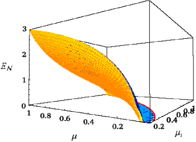
Fig. 3: Maximal and minimal logarithmic negativity as functions of the global and marginal purities of symmetric Gaussian states. The darker (lighter) surface represents GMEMS (GLEMS).

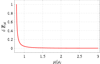
Fig. 4: Plot of relative error $\delta\bar{E}_{{\cal N}}$ on the average logarithmic negativity as a function of the ratio $\mu/\mu_{i}$ ($\mu=0.5$).

In Fig. 4, $E_{{{\cal N}}max}(\mu_{i},\,\mu)$ of Eq. (21) and $E_{{{\cal N}}min}(\mu_{i},\,\mu)$ of Eq. (22) are plotted versus $\mu_{i}$ and $\mu$. In the case $\mu=1$ the upper and lower bounds correctly coincide, since for pure states the entanglement is completely quantified by the marginal purity. For mixed states this is not the case, but, as the plot shows, knowledge of the global and marginal purities strictly bounds the entanglement both from above and from below. The relative error $\delta\bar{E}_{{\cal N}}(\mu_{i},\,\mu)$ given by Eq. (24) is plotted in Fig. 4 as a function of the ratio $\mu/\mu_{i}$. It decays exponentially, dropping below $5\%$ for $\mu>\mu_{i}$. Thus the reliable quantification of quantum correlations in genuinely entangled states is always assured by this method, except at most for a small set of states with very weak entanglement (states with $E_{{\cal N}}\lesssim 1$). Moreover, the accuracy is even greater in the general non-symmetric case $\mu_{1}\neq\mu_{2}$, because the maximal entanglement decreases in such an instance (see Fig. 1). This analysis shows that the average logarithmic negativity $\bar{E}_{{\cal N}}$ is a reliable estimate of the logarithmic negativity $E_{{\cal N}}$, improving as the entanglement increases. This allows for an accurate quantification of CV entanglement by knowledge of the global and marginal purities. The purities may be in turn directly measured experimentally, without the full tomographic reconstruction of the whole CM, by exploiting quantum networks techniques [30] or single–photon detections without homodyning [31, 32].

3.5. Entanglement vs Information (IV) – Extremal entanglement at fixed global and local generalized entropies

In this section we introduce a more general characterization of the entanglement of two–mode Gaussian states in terms of the degrees of information, by exploiting the generalized Tsallis $p-$entropies

$$S_{p}\equiv\frac{1-\,{\rm Tr}\,\varrho^{p}}{p-1}\;,\quad p>1,$$ (25)

as measures of global and marginal mixedness. Such an analysis can be carried out along the same lines of the previous section, by studying the explicit behavior of the global invariant $\Delta$ at fixed global and marginal entropies, and its relation with the logarithmic negativity $E_{\cal N}$. Let us remark that the $S_{p}$’s can be computed for a generic Gaussian state in terms of the symplectic eigenvalues [18], namely

$${\rm Tr}\,\varrho^{p}=\prod_{i=1}^{n}g_{p}(\nu_{i})\;,\quad g_{p}(x)=\frac{2^{p}}{(x+1)^{p}-(x-1)^{p}}\,.$$ (26)

We begin by observing that the standard form CM $\boldsymbol{\sigma}$ of a generic two–mode Gaussian state Eq. (4) can be parametrized by the following quantities: the two marginals $\mu_{1,2}$ (or any other marginal $S_{p_{1,2}}$ because all the local, single-mode entropies are equivalent for any value of the integer $p$), the global $p-$entropy $S_{p}$ (for some chosen value of the integer $p$), and the global symplectic invariant $\Delta$.

After somewhat lengthy but straightforward calculations (the details can be found in Ref. [18]), one finds that the entanglement is still bounded from above and from below by functionals of the global and marginal $p-$entropies, and the two extremal classes of states are again the nonsymmetric squeezed thermal states (GMEMS) and the mixed states of partial minimum uncertainty (GLEMS). Nevertheless, the seralian $\Delta$ is no longer monotonically related to the entanglement of the state, at fixed generalized entropies. In particular, for any $p>2$ (i.e. with the exception of the linear and Von Neumann entropies), there exists a unique nodal surface ${\cal S}_{p}^{n}(S_{p_{1,2}})$ such that

$$\left.\frac{\partial\,\tilde{\nu}_{-}}{\partial\,\Delta}\right|_{S_{p_{1}},S_{p_{2}},S_{p}}\quad{\rm is}\quad\left\{\begin{array}[]{ll}>0,&\hbox{ when}\quad S_{p}>{\cal S}_{p}^{n}(S_{p_{1,2}})\,;\\ =0,&\hbox{ when}\quad S_{p}={\cal S}_{p}^{n}(S_{p_{1,2}})\,;\\ <0,&\hbox{ when}\quad S_{p}<{\cal S}_{p}^{n}(S_{p_{1,2}})\,.\\ \end{array}\right.$$ (27)

While in the first case of Eq. (27) GMEMS and GLEMS retain their property of being, respectively, maximally and minimally entangled Gaussian states for fixed degrees of information, in the last case they exchange their role: two–mode squeezed states become minimally entangled states for fixed $p-$entropies, and the states of partial minimum uncertainty are those with maximal entanglement. Even more remarkably, the entanglement of all Gaussian states (including GMEMS, GLEMS and infinitely many other different states) whose $p-$entropies lay on the nodal surface of inversion $S_{p}={\cal S}_{p}^{n}(S_{p_{1,2}})$, does not depend on $\Delta$ and is therefore completely quantified in terms of the global and marginal generalized degrees of information. Thus the state parametrization by the Tsallis $p-$entropies (and, presumably, by the companion family of the Rényi entropies [33] as well), provides a remarkable inversion between GMEMS and GLEMS, and allows to identify a class of Gaussian states whose entanglement is quantified exactly by the knowledge of the global and marginal degrees of information. Moreover, even outside the nodal surface of inversion, the gap between maximal and minimal entanglement for fixed $p-$entropies decreases with increasing $p$, so that the accuracy of the quantitative estimate of the logarithmic negativity as a function of the $p-$entropies increases accordingly, as shown in Fig. 5. Despite this interesting features, measurements of purity, or equivalently of linear entropy ($p=2$), remain the best candidates for a direct estimation of CV entanglement in realistic experiments. This is due to the fact that measuring the global $p-$entropy ($p\neq 2$) of a state requires the full tomographic reconstruction of the whole CM, thus nullifying the advantages of the analysis presented in Sec. 3.4..

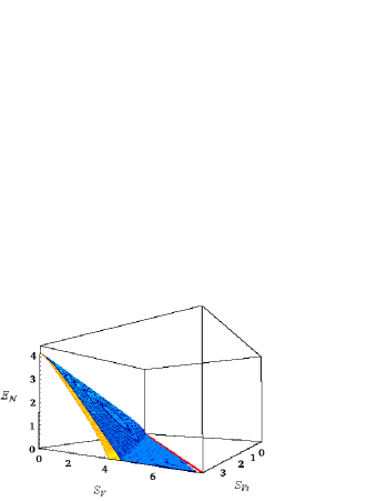
(a)

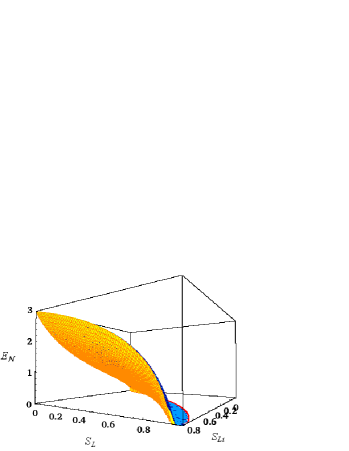
(b)

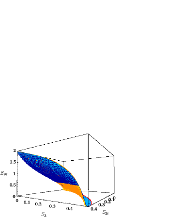
(c)

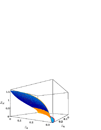
(d)

Fig. 5: Lower and upper bounds on the logarithmic negativity of symmetric Gaussian states as functions of the global and marginal generalized $p-$entropies, for (a) $p\rightarrow 1$ (von Neumann entropies), (b) $p=2$ (linear entropies), (c) $p=3$, and (d) $p=4$. The darker (lighter) surfaces represent GMEMS (GLEMS). Notice that for $p>2$ GMEMS and GLEMS surfaces intersect along the nodal inversion line (meaning they are equally entangled along that line), and beyond it they interchange their role.

4. Quantification of multimode entanglement under symmetry

For two–mode Gaussian states of CV systems we have shown that the measurement of the three purities (or generalized entropies), out of the four independent standard form covariances, suffices in providing a reliable quantitative characterization of the entanglement. It is intuitively evident that the efficiency of such a quantitative estimation in terms of information entropies should improve significantly with increasing number $N$ of modes, because the ratio between the total number of covariances and the total number of global and marginal degrees of information quickly scales with $N$. Moreover, the structure of multipartite entanglement that can arise in multimode settings is much richer than the basic bipartite CV entanglement. Here we briefly discuss the simplest multipartite setting in which the purities again successfully bound the entanglement with great accuracy.

We consider highly symmetric $(N+1)$-mode Gaussian states of generic single-mode systems $\boldsymbol{\alpha}$ coupled to fully symmetric $N$-mode systems $\boldsymbol{\sigma}_{\beta^{N}}$, resulting in a global CM $\boldsymbol{\sigma}$ of the form

$$\boldsymbol{\sigma}\!=\!\left(\!\begin{array}[]{cc}\boldsymbol{\alpha}&\boldsymbol{\Gamma}\\ \boldsymbol{\Gamma}^{\sf T}&\boldsymbol{\sigma}_{\beta^{N}}\\ \end{array}\right)\!,\quad\boldsymbol{\sigma}_{\beta^{N}}=\left(\begin{array}[]{cccc}\boldsymbol{\beta}&\boldsymbol{\varepsilon}&\cdots&\boldsymbol{\varepsilon}\\ \boldsymbol{\varepsilon}&\boldsymbol{\beta}&\boldsymbol{\varepsilon}&\vdots\\ \vdots&\boldsymbol{\varepsilon}&\ddots&\boldsymbol{\varepsilon}\\ \boldsymbol{\varepsilon}&\cdots&\boldsymbol{\varepsilon}&\boldsymbol{\beta}\\ \end{array}\right)\!,\quad\boldsymbol{\Gamma}=(\underbrace{\boldsymbol{\gamma}\;\cdots\;\boldsymbol{\gamma}}_{N})\,.$$ (28)

The state $\boldsymbol{\sigma}$ is determined by six independent parameters, three of which are related to the fully symmetric $N$-mode block $\boldsymbol{\sigma}_{\beta^{N}}$ (or, equivalently, to any of its two–mode subblocks $\boldsymbol{\sigma}_{\beta^{2}}$). The remaining parameters are determined by the single-mode purity $\mu_{\alpha}\equiv({\rm Det}\,\boldsymbol{\alpha})^{-1/2}$ and by the two global $Sp_{(2N+2,\mathbbm{R})}$ invariants ${\rm Det}\,\boldsymbol{\sigma}\equiv 1/(\mu_{\sigma}^{2})=\prod_{i=1}^{N+1}\nu_{i}^{2}$ and $\Delta_{\sigma}\equiv\Delta_{\alpha}+\Delta_{\beta^{N}}=\sum_{i=1}^{N+1}\nu_{i}^{2}$. Here $\mu_{\sigma}$ is the global purity of the state $\boldsymbol{\sigma}$, the $\nu_{i}$’s constitute its symplectic spectrum, $\Delta_{\alpha}\equiv{\rm Det}\,\boldsymbol{\alpha}+2N{\rm Det}\,\boldsymbol{\gamma}$, and $\Delta_{\beta^{N}}\equiv N({\rm Det}\,\boldsymbol{\beta}+(N-1){\rm Det}\,\boldsymbol{\varepsilon})$.

To compute the multimode $1\times N$ logarithmic negativity of state $\boldsymbol{\sigma}$ between the mode $\boldsymbol{\alpha}$ and the $N$-mode block $\boldsymbol{\sigma}_{\beta^{N}}$, it is convenient to perform the local symplectic operation that brings $\boldsymbol{\sigma}_{\beta^{N}}$ in its Williamson normal form, which is characterized by a $(N-1)$-times degenerate eigenvalue $\nu_{-}=\sqrt{(b-e_{1})(b-e_{2})}$ (the same smallest symplectic eigenvalue of the two–mode subblock $\boldsymbol{\sigma}_{\beta^{2}}$) and a nondegenerate eigenvalue $\nu_{+^{(N)}}=\sqrt{(b+(N-1)e_{1})(b+(N-1)e_{2})}=1/(\nu_{-}^{N-1}\mu_{\beta^{N}})$, where $\mu_{\beta^{N}}$ is the purity of the $N$-mode fully symmetric block [16]. The crucial point here is that this local operation actually decouples the mode $\boldsymbol{\alpha}$ from all the $(N-1)$ modes corresponding to the eigenvalue $\nu_{-}$ and concentrates the whole $1\times N$ entanglement between only two modes. The state Eq. (28) is thus brought in the form $\boldsymbol{\sigma}=\left(\begin{array}[]{cc}\boldsymbol{\sigma}^{eq}&{\bf 0}\\ {\bf 0}&\boldsymbol{\nu}_{-}\\ \end{array}\right),$ where $\boldsymbol{\nu}_{-}$ is a diagonal $(2N-2)\times(2N-2)$ matrix with all entries equal to $\nu_{-}$, and the equivalent two–mode state $\boldsymbol{\sigma}^{eq}$ is characterized by its invariants

$$\mu_{1}^{eq}=\mu_{\alpha},\quad\mu_{2}^{eq}=\nu_{-}^{N-1}\mu_{\beta^{N}},\quad\mu^{eq}=\nu_{-}^{N-1}\mu_{\sigma},\quad\Delta^{eq}=\Delta_{\alpha}+(\nu_{-}^{N-1}\mu_{\beta^{N}})^{-2}\,.$$ (29)

These invariants are, in turn, determined in terms of the six invariants of the original $N$-mode state $\boldsymbol{\sigma}$, but we can exploit the previous two–mode analysis (see Sec. 3.4.) to conclude that, even without the explicit knowledge of $\Delta^{eq}$, and so of the coupling ${\rm Det}\,\boldsymbol{\gamma}$, the multimode entanglement under symmetry can be quantified through the average logarithmic negativity Eq. (23) of the equivalent state $\boldsymbol{\sigma}^{eq}$, with the same accuracy demonstrated for generic two–mode states (see Fig. 4).

Thus the degrees of information of a multipartite Gaussian state again provide a strong characterization and a reliable quantitative estimate of the entanglement. Moreover, the method of the two–mode reduction can be used to compute the $1\times K$ entanglement between the mode $\boldsymbol{\alpha}$ and any $K-$mode subblock of $\boldsymbol{\sigma}_{\beta^{N}}$, with $K=1,\ldots,N$, in order to establish a multipartite entanglement hierarchy in the $(N+1)$-mode state of the form Eq. (28) [34].

5. Summary and Outlook

In this work we aimed at unveiling the close relation between the entanglement encoded in a quantum state and its degrees of information. We have shown in detail how the knowledge of the global degree of information alone, or of the marginal informations related to the subsystems of a multipartite system, results in a qualitative characterization of the entanglement: the latter increases with decreasing global mixedness, with increasing marginal mixednesses, and with marginal mixednesses as close as possible. We then proved how the simultaneous knowledge of all the global and local degrees of information of a Gaussian state leads to the identification of extremally (maximally and minimally) entangled states at fixed mixednesses (purities or generalized information entropies), providing an accurate quantitative characterization of CV entanglement. It is worth remarking that, out of the subset of Gaussian states, very little is known about entanglement and information in generic states of CV systems. Nevertheless, most of the results presented here (including the sufficient conditions for entanglement based on information measures), derived for CM’s using the symplectic formalism in phase space, retain their validity for generic states of CV systems. For instance, any two-mode state with a CM corresponding to an entangled Gaussian state is itself entangled too [35]. So our methods may serve to detect entanglement in a broader class of states of infinite-dimensional Hilbert spaces.

The generalization of this analysis, connecting entanglement and information, to highly symmetric multimode Gaussian states of $1\times N$-mode partitions has been briefly sketched, presenting a simple method to estimate CV multimode entanglement by measurements of purity in an equivalent two–mode state. The extension of this method to the quantification of multipartite entanglement in Gaussian states with respect to generic $M\times N$ bipartitions of the modes [36], as well as a deeper understanding of the structure of genuine multipartite CV entanglement [37] and its relation with multiple degrees of information beyond the symmetry constraints, are being currently investigated.

References

- [1] E. Schrödinger, Discussion of probability relations between separated systems (I), Proceedings of the Cambridge Philosophical Society, vol. 31 (1935), p. 555.
- [2] M. A. Nielsen and I. L. Chuang, Quantum Computation and Quantum Information (Cambridge University Press, Cambridge, 2000).
- [3] L. Henderson and V. Vedral, Phys. Rev. Lett. 84, 2263 (2000).
- [4] Quantum Information Theory with Continuous Variables, S. L. Braunstein and A. K. Pati Eds. (Kluwer, Dordrecht, 2002).
- [5] S. L. Braunstein and P. van Loock, quant-ph/0410100, and Rev. Mod. Phys., to appear.
- [6] R. Simon, E. C. G. Sudarshan, and N. Mukunda, Phys. Rev. A 36, 3868 (1987).
- [7] J. Williamson, Am. J. Math. 58, 141 (1936); see also V. I. Arnold, Mathematical Methods of Classical Mechanics, (Springer-Verlag, New York, 1978).
- [8] A. Serafini, F. Illuminati, and S. De Siena, J. Phys. B: At. Mol. Opt. Phys. 37, L21 (2004).
- [9] M. G. A. Paris, F. Illuminati, A. Serafini, and S. De Siena, Phys. Rev. A 68, 012314 (2003).
- [10] M. J. Bastiaans, J. Opt. Soc. Am. 1, 711 (1984); ibid. 3, 1243 (1986).
- [11] C. Tsallis, J. Stat. Phys. 52, 479 (1988).
- [12] A. Rényi, Probability Theory (North Holland, Amsterdam, 1970).
- [13] A. Peres, Phys. Rev. Lett. 77, 1413 (1996); R. Horodecki, P. Horodecki, and M. Horodecki, Phys. Lett. A 210, 377 (1996).
- [14] R. Simon, Phys. Rev. Lett. 84, 2726 (2000).
- [15] G. Vidal and R. F. Werner, Phys. Rev. A 65, 032314 (2002); K. Życzkowski, P. Horodecki, A. Sanpera, and M. Lewenstein, Phys. Rev. A 58, 883 (1998); J. Eisert, PhD Thesis, (University of Potsdam, Potsdam, 2001).
- [16] G. Adesso, A. Serafini, and F. Illuminati, Phys. Rev. Lett. 93, 220504 (2004).
- [17] L.-M. Duan, G. Giedke, J. I. Cirac, and P. Zoller, Phys. Rev. Lett. 84, 2722 (2000).
- [18] G. Adesso, A. Serafini, and F. Illuminati, Phys. Rev. A 70, 022318 (2004).
- [19] The largest eigenvalue of the partially transposed CM of a two–mode Gaussian state is always greater than 1 and so it does not enter in the computation of the logarithmic negativity Eq. (2), see Ref. [18].
- [20] C. H. Bennett, D. P. DiVincenzo, J. A. Smolin, and W. K. Wootters, Phys. Rev. A 54, 3824 (1996).
- [21] G. Giedke, M. M. Wolf, O. Krüger, R. F. Werner, and J. I. Cirac, Phys. Rev. Lett. 91, 107901 (2003).
- [22] S. Ishizaka and T. Hiroshima, Phys. Rev. A 62, 022310 (2000).
- [23] F. Verstraete, K. Audenaert, and B. De Moor, Phys. Rev. A 64, 012316 (2001); W. J. Munro, D. F. V. James, A. G. White, and P. G. Kwiat, Phys. Rev. A 64, 030302 (2001).
- [24] T.-C. Wei, K. Nemoto, P. M. Goldbart, P. G. Kwiat, W. J. Munro, and F. Verstraete, Phys. Rev. A 67, 022110 (2003).
- [25] J. Eisert and M. Plenio, J. Mod. Opt. 46, 145 (1999); F. Verstraete, K. Audenaert, J. Dehaene, and B. de Moor, J. Phys. A 34, 10327 (2001).
- [26] K. Życzkowski, P. Horodecki, A. Sanpera and M. Lewenstein, Phys. Rev. A 58, 883 (1998); K. Życzkowski, Phys. Rev. A 60, 3496 (1999).
- [27] G. Adesso, F. Illuminati, and S. De Siena, Phys. Rev. A 68, 062318 (2003).
- [28] W. K. Wootters, Phys. Rev. Lett. 80, 2245 (1998).
- [29] G. Adesso, A. Serafini, and F. Illuminati, Phys. Rev. Lett. 92, 087901 (2004).
- [30] A. K. Ekert, C. M. Alves, D. K. L. Oi, M. Horodecki, P. Horodecki, and L. C. Kwek, Phys. Rev. Lett. 88, 217901 (2002); R. Filip, Phys. Rev. A 65, 062320 (2002).
- [31] J. Fiurás̆ek and N. J. Cerf, Phys. Rev. Lett. 93, 063601 (2004).
- [32] J. Wenger, J. Fiurás̆ek, R. Tualle-Brouri, N. J. Cerf, and Ph. Grangier, Phys. Rev. A 70, 053812 (2004).
- [33] K. Życzkowski, Open Systems & Information Dynamics 10, 297 (2003).
- [34] Being all equivalent to two–mode entanglements, all the entanglements can be directly compared to each other. For furter details see Ref. [16].
- [35] P. van Loock, Fortschr. Phys. 50, 12 1177 (2002).
- [36] A. Serafini, G. Adesso, and F. Illuminati, Phys. Rev. A 71, 032349 (2005).
- [37] G. Adesso and F. Illuminati, quant-ph/0410050 (2004).