Evanescence in Coined Quantum Walks

Hilary A. Carteret
Laboratoire d’Informatique Théorique et Quantique,
Département d’Informatique et de Recherche Opérationelle,
Pavillon André-Aisenstadt,
Université de Montréal,
Montréal, Québec, H3C 3J7
Canada
email: cartereh@iro.umontreal.ca
   Bruce Richmond
Department of Combinatorics and Optimization
University of Waterloo
Waterloo, Ontario, N2L 3G1
Canada
email: lbrichmo@hopper.math.uwaterloo.ca
   Nico M. Temme
CWI
Kruislaan 413, NL-1098, SJ Amsterdam,
Netherlands,
email: Nico.Temme@cwi.nl
($10^{{\rm{th}}}$ August, 2005)
Abstract

In this paper we complete the analysis begun by two of the authors in a previous work on the discrete quantum walk on the infinite line [J. Phys. A 36:8775-8795 (2003); quant-ph/0303105]. We obtain uniformly convergent asymptotics for the “exponential decay” regions at the leading edges of the main peaks in the Schrödinger (or wave-mechanics) picture. This calculation required us to generalise the method of stationary phase and we describe this extension in some detail, including self-contained proofs of all the technical lemmas required. We also rigorously establish the exact Feynman equivalence between the path-integral and wave-mechanics representations for this system using some techniques from the theory of special functions. Taken together with the previous work, we can now prove every theorem by both routes.

1 Introduction

The first authors to discuss the quantum walk were Aharonov, Davidovich and Zagury in [4] where they described a very simple realization in quantum optics. In this model a particle takes unit steps on the integers at each time step, starting at the origin. In [28] Meyer proved that an additional spin-like degree of freedom was essential if the behaviour of the system was to be both unitary and non-trivial. Without this degree of freedom, the only way the evolution of the walk can avoid being purely ballistic is to relax the unitarity condition. This spin-like degree of freedom is sometimes called the chirality, or the coin, which is why this type of walk is sometimes called a “coined” walk [35]. This is in sharp contrast to the continuous time walk [14, 13] which does not need a coin and which we will not discuss here. The chirality can take the values RIGHT and LEFT, or a coherent superposition of these.

Refer to caption
Figure 1: The discrete quantum walk on the line. The probability distribution is shown for a walk that started at the origin with its coin in the state $|\rm{L}\rangle$ after it has evolved for 100 steps. The distribution is oscillatory between the two peaks and decays exponentially outside that range. The peaks move away from the origin with speed $t/\sqrt{2},$ and the width of the peaks also decreases with time. By contrast, the classical random walk has a Gaussian distribution, which spreads with velocity $\sim\sqrt{t}.$

For a detailed introduction to quantum walks, we refer the reader to the review article in [21].

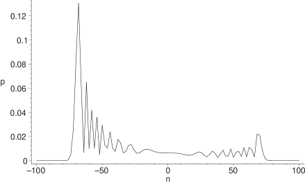
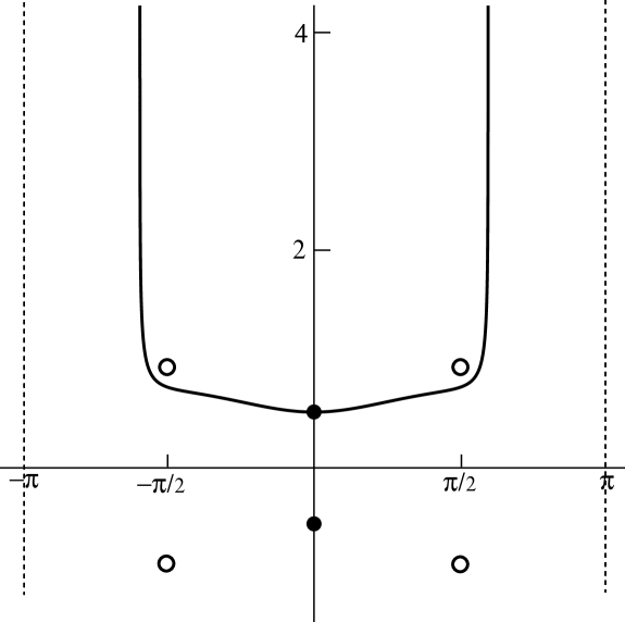
Meyer and subsequent authors [2, 5] have considered two approaches to the discrete-time quantum walk, the path-integral approach of Feynman and the Schrödinger wave-mechanics approach, which reflect two complementary ways of formulating quantum mechanics [15]. We refer to the paper by Ambainis, Bach, Nayak, Vishwanath and Watrous [5] for proper definitions and more references. Both approaches are discussed in the paper of Ambainis et al. The probability distribution for this walk is shown in Figure 1, after enough time has elapsed for the asymptotic behaviour to manifest.

This paper began as a sequel to the work of Carteret, Ismail and Richmond [10] concerning the one-dimensional quantum walk on the integers, and contains the completion of the analysis of this quantum walk for the remaining exponential decay region in the Schrödinger picture. We believe the analysis presented in this paper to be interesting for three reasons. One is methodological; while analysing this system we encountered various links between a number of different methods in combinatorics which do not seem to be widely known, and which may be of use to the quantum information community when analysing more complicated systems than the one discussed here.

The second motivation is rather more abstract. It is one of the fundamental principles of quantum mechanics that the wave-mechanics and path-integral representations of a system should produce exactly the same results. The quantum walk has been proposed as the quantum analogue of the classical random walk, in the hopes of ultimately defining a systematic procedure for “quantizing” classical random walk algorithms [21, 6, 33]. Quantizing classical systems is something that must be done with considerable care; the obvious approach isn’t necessarily the correct one. While it is true that when such pathologies have been discovered in the past, they were found in much more exotic systems than this one, it is as well to check. One way to perform such a check is to verify that the Feynman equivalence principle still holds between the path-integral and wave-mechanics representations. As it happens, the results obtained from the two approaches do not at first appear to be equivalent. In fact they are, though the proof of their equivalence is nontrivial, and will be given in Section 3. In the course of this analysis we uncovered a small, but potentially significant omission in previous analyses of this system, which we will describe below.

Another reason for performing this check is to explore the little mystery left at the end of [10]. While the results from the path integral calculation made intuitive sense, the partial results from the wave-mechanics calculation for the exponential decay region were rather unexpected. Specifically, we found what appeared to be evanescent waves in this exponential decay region, which seemed to imply the presence of some kind of absorption mechanism, despite the fact that the definition of the model precludes any barrier or other source of dissipation in the system to cause these by the familiar mechanisms. So, we will check that the Feynman equivalence holds to verify that those evanescent waves are not simply some kind of mathematical artefact.

We would also like to gain some insight into the physical interpretation of the mathematical behaviour of this part of the wave-function. A link between the behaviour of the quantum walk on the line and certain phenomena in quantum optics has been suggested previously by Knight, Roldan and Sipe in [25, 24, 26], and refined by Kendon and Sanders in [23]. This connection will be discussed in more detail in Section 4.

We will also describe a potentially useful method for obtaining integral representations of orthogonal polynomials from their generating functions using Lagrange Inversion. This bypasses the need to use the Darboux method and makes it possible to obtain uniformly convergent asymptotics directly from the generating function. We have included this in the Appendices in Subsection 6.2.

1.1 Some previous results

In this section we will mention some results by other authors which we will have occasion to use later in this paper. One of the reasons for doing this is that different authors have used different labelling conventions and this will enable us to establish a consistent notation for use when we combine results from different papers with mutually incompatible conventions. We will state our results using the conventions in [10].

Several early results in the theory of quantum walks are due to Meyer [28], who considered the wavefunction as a two-component vector of amplitudes of the particle being at point $n$ at time $t$. Let

$$\Psi(n,t)=\begin{pmatrix}\psi_{R}(n,t)\\ \psi_{L}(n,t)\end{pmatrix}$$ (1)

where the chirality of the top component is labelled RIGHT and the bottom LEFT. At each step the chirality of the particle evolves according to a unitary Hadamard transformation

$\displaystyle|R\rangle$ $\displaystyle\mapsto\frac{1}{\sqrt{2}}\left(|R\rangle+|L\rangle\right)$ (2)
$\displaystyle|L\rangle$ $\displaystyle\mapsto\frac{1}{\sqrt{2}}\left(|R\rangle-|L\rangle\right),$ (3)

which is why this quantum walk is sometimes called the “Hadamard” walk. The particle (or “walker”) then moves according to its new chirality state. Therefore, the particle obeys the recursion relations

$\displaystyle\Psi_{R}(n,t+1)$ $\displaystyle=\frac{1}{\sqrt{2}}\Psi_{L}(n+1,t)+\frac{1}{\sqrt{2}}\Psi_{R}(n-1,t)$ (4)
$\displaystyle\Psi_{L}(n,t+1)$ $\displaystyle=-\frac{1}{\sqrt{2}}\Psi_{L}(n+1,t)+\frac{1}{\sqrt{2}}\Psi_{R}(n-1,t).$ (5)

Meyer approached this problem from the path-integral point of view, and obtained expressions for the $\psi$-functions in terms of Jacobi polynomials. The standard notation in [1] for Jacobi polynomials is $P_{n}^{(\alpha,\beta)}(z)$ but we wish to follow the conventions in [29] and subsequent papers that have now become standard in the literature on quantum walks, and use $\alpha=n/t.$ We will therefore use the notation $J_{q}^{(r,s)}(w).$

We find, in [5] and [10] when $n\neq t$,

Theorem 1 (Ambainis et al. [5], after Meyer, [28]).
$$\psi_{R}(n,t)(-1)^{(t-n)/2}=\begin{cases}2^{n/2-1}J_{((t+n)/2-1)}^{(1,-n)}(0)&\text{when }-t\leq n<0\\ \left(\frac{t+n}{t-n}\right)2^{-n/2-1}J_{(t-n)/2-1}^{(1,n)}(0)&\text{when }0\leq n<t\end{cases}$$ (6)

Also

$$\psi_{L}(n,t)(-1)^{(t-n)/2}=\begin{cases}2^{n/2}J_{(t+n)/2}^{(0,-n-1)}(0)&\text{when }-t\leq n<0\\ 2^{-n/2-1}J_{(t-n)/2-1}^{(0,n+1)}(0)&\text{when }0\leq n<t\end{cases}$$ (7)

and

$\displaystyle|\psi_{R}(n,t)|^{2}$ $\displaystyle=\left(\frac{t-n}{t+n}\right)^{2}|\psi_{R}(-n,t)|^{2}$ (8)
$\displaystyle|\psi_{L}(n,t)|^{2}$ $\displaystyle=|\psi_{L}(2-n,t)|^{2}.$ (9)

Ambainis et al. use the other sign convention, so one should interchange $L$ and $R$ (or equivalently, replace $n$ by $-n$) to reflect the walk before comparing their results with ours. This is just a relabelling, and so their results can be stated as in the following theorem. We will prove the above results in the form below

Theorem 2 (Ambainis et al. [5]).

When $n\equiv t\,({\rm{mod}}\,2)$ and $J_{q}^{(r,s)}(w)$ denotes a Jacobi polynomial, then

$$\psi_{R}(n,t)(-1)^{(t-n)/2}=\begin{cases}(-1)^{n+1}2^{-n/2}J_{(t-n)/2}^{(0,n-1)}(0)&\text{when }0\leq n\leq t\\ (-1)^{n+1}2^{n/2-1}J_{(t+n)/2-1}^{(0,-n+1)}(0)&\text{when }-t<n<0\end{cases}$$ (10)

Also

$$\psi_{L}(n,t)(-1)^{(t-n)/2}=\begin{cases}-2^{-n/2-1}J_{(t-n)/2-1}^{(1,n)}(0)&\text{when }0\leq n<t\\ -\left(\frac{t-n}{t+n}\right)2^{n/2-1}J_{(t+n)/2-1}^{(1,-n)}(0)&\text{when }-t<n<0.\end{cases}$$ (11)

and

$\displaystyle\psi_{R}(-n,t)$ $\displaystyle=(-1)^{n+1}\psi_{R}(n+2,t),$ (12)
$\displaystyle(t-n)\psi_{L}(-n,t)$ $\displaystyle=(-1)^{n}(t+n)\psi_{L}(n,t).$ (13)

A few Remarks:

  1. 1.

    Note that Theorem 2 differs from Theorem 1 by an external phase which has been dropped in previous analyses of this system; we state the symmetry relations for the $\psi$-functions rather than for their moduli-squared, as in [5]. We will discuss this in more detail below, as some properties of Jacobi polynomials are required for the calculation.

  2. 2.

    There is a sign error in the symmetry relations for $\psi_{R}$ and $\psi_{L}(-n,t)$ in Carteret et al. [10] (which has been corrected in the arxiv version [11]). The symmetry relations will be proved in Lemmas 2, 3 and equation (77) of Subsection 3.1 using some integral representations of $\psi_{R}(n,t)$ and $\psi_{L}(n,t)$.

  3. 3.

    The endpoints where $n=\pm t$ have to be handled separately, see [28]. For the starting conditions

    $\displaystyle\psi_{L}(0,0)=1,$ $\displaystyle\psi_{R}(0,0)=0$

    the wavefunctions at the end-points (where $n=\pm t$) are

    $\displaystyle\psi_{R}(t,t)$ $\displaystyle=(-1)^{t+1}2^{-t/2}$ $\displaystyle t=0,1,2,\ldots,$ (14)
    $\displaystyle\psi_{L}(t,t)$ $\displaystyle=0,$ $\displaystyle t=1,2,3,\ldots,$ (15)
    $\displaystyle\psi_{R}(-t,t)$ $\displaystyle=0,$ $\displaystyle t=1,2,3,\ldots,$ (16)
    $\displaystyle\psi_{L}(-t,t)$ $\displaystyle=(-1)^{t}2^{-t/2},$ $\displaystyle t=0,1,2,\ldots.$ (17)
  4. 4.

    The two different cases in (11) and (10) for $n\geq 0$ and $n<0$ can be combined into one case for all $n$ satisfying $-t\leq n<t.$ We prove this later using a symmetry property of the Jacobi polynomials. Our results in equations (12) and (13) are refinements of the corresponding relations in (9) and (8), after performing the relabelling necessary to compare results with different sign conventions.

The asymptotic behaviour for the path-integral representation has been determined in Carteret et al. [10], starting from Theorem 2. The steepest descent technique was used on the standard integral representation for the Jacobi polynomial. The result was uniform exact asymptotics $\alpha$ in the range $|\alpha|<1-\varepsilon,$ where $\varepsilon$ is any positive number, in terms of Airy functions.

This technique was used earlier for Jacobi polynomials by Saff and Varga [31] and by Gawronkski and Sawyer [18]; however the connection with Airy functions had not been recognized as far as we know. The Airy function description is useful for $|\alpha|$ near $1/\sqrt{2}$ where the asymptotic behaviour changes from an oscillating cosine term times $t^{-1/2}$ (for $|\alpha|<1/\sqrt{2}$) to exponentially small (for $2^{-1/2}+\varepsilon<|\alpha|<1-\varepsilon).$


In this paper we analyze the Hadamard walk from the Schrödinger wave-mechanics point of view. The earliest work on this that the authors are aware of is that by Nayak and Vishwanath [29]. They define

$$\widetilde{\Psi}(\theta,t)=\sum_{n}\psi(n,t)e^{i\theta n},$$ (18)

(where we have used the symbol $\theta$ for the momentum instead of the $k$ used in [29]) so the recursion relations above becomes

$$\widetilde{\Psi}(\theta,t+1)=M_{\theta}\widetilde{\Psi}(\theta,t),$$ (19)

where

$$M_{\theta}=\begin{pmatrix}e^{-i\theta}&e^{-i\theta}\\ e^{i\theta}&-e^{i\theta}\end{pmatrix}\,.$$ (20)

Thus

$$\widetilde{\Psi}(\theta,t)=M_{\theta}^{t}\widetilde{\Psi}(\theta,0),\quad\widetilde{\Psi}(\theta,0)=(1,0)^{{\rm{T}}},$$ (21)

where the symbol $\;{}^{{\rm{T}}}$ denotes transposition. They show that the eigenvalues of $M_{\theta}$ are $e^{-i\omega_{\theta}}$ and $-e^{i\omega_{\theta}}$ where $\omega_{\theta}$ is the angle in $[-\pi/2,\pi/2]$ such that $\sin(\omega_{\theta})=(\sin\theta)/\sqrt{2}.$ They also use the other sign convention, so one should relabel $L$ and $R$ as before. Their results can be stated as in the following theorem.

Theorem 3 (Nayak and Vishwanath [29]).

Let $\alpha=n/t$. Then

$$\psi_{R}(n,t)=\frac{1+(-1)^{n+t}}{2}\frac{1}{2\pi}\int_{-\pi}^{\pi}\frac{e^{i\theta}}{\sqrt{1+\cos^{2}\theta}}e^{-i(\omega_{\theta}+\theta\alpha)t}\;d\theta.$$ (22)
$$\psi_{L}(n,t)=\frac{1+(-1)^{n+t}}{2}\frac{1}{2\pi}\int_{-\pi}^{\pi}\left(1+\frac{\cos\theta}{\sqrt{1+\cos^{2}\theta}}\right)e^{-i(\omega_{\theta}+\theta\alpha)t}\;d\theta,$$ (23)

We will derive the asymptotic behaviour of the $\psi$-functions starting from Theorem 3 in Section 2. We will only give the complete details for the exponential decay range, as the calculation for the oscillatory region has already been done by others [29, 5]. The conventional version of the method of stationary phase, as used by Nayak-Vishwanath [29], does not work in the exponentially small region, as the stationary points of the phase function have left the real line. We will show how to extend and refine this technique so that it can be made to work in this situation; the modification is an application of the method of steepest descents.

It is not obvious that the formulæ  obtained by each method are the same, but we will prove below in Section 3 that they are. This means that precisely the same asymptotic behaviour can be found using both the path-integral and wave-mechanics descriptions of quantum mechanics.

2 Generalizing the method of stationary phase

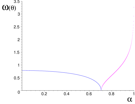
The aim of this section is to extend the method of stationary phase so that it can cope with stationary points that occur as complex conjugate pairs on either side of the real axis. We start with the integral representation of $\psi_{R}$ in Theorem 3. In this representation the integration is performed along the real axis. Nayak and Vishwanath consider the case $|\alpha|<1/\sqrt{2}$ when there are two stationary points (defined below) inside the interval of integration $[-\pi,\pi]$. When we find the critical points of the phase function, we obtain an equation for $\theta$ (called $k$ in [10]) at the critical points as a function of $\alpha,$ which is

$$\cos\theta_{\alpha}=\frac{-\alpha}{\sqrt{1-\alpha^{2}}}$$ (24)

from which the critical value of $\omega_{\theta},$ call it $\omega_{{\theta}_{\alpha}},$ can be obtained using the Pythagoras rule ($\cos^{2}\theta+\sin^{2}\theta=1$) and $\omega_{\theta}=\arcsin\frac{\sin\theta}{\sqrt{2}}$ from [29]. However, when $|\alpha|>1/\sqrt{2}$ this equation no longer has any real solutions and thus the corresponding stationary points are no longer on the real axis, see figure 2. Therefore the standard method of stationary phase cannot provide the exact asymptotics. The stationary points have “moved” off the real axis and become a complex conjugate pair. We shall move the contour of integration to follow the stationary points, whilst ensuring that the contour still goes through one of them. Note also that the stationary points become saddle-points on leaving the real line; we will return to this fact in Subsection 2.2, below.

Refer to caption
Figure 2: The behaviour of $\omega_{\theta}$ as $|\alpha|>1/\sqrt{2}.$ As $|\alpha|$ moves beyond the critical value of $1/\sqrt{2}$, the phase function $\omega_{\theta}$ becomes imaginary. The behaviour of the real part is shown in the solid line and that of the nascent imaginary part is shown in the dotted line. Multiplying this imaginary phase function by $i$ gives a simple exponential decay.

2.1 The function ${\boldsymbol{\omega_{\theta}}}$ in the complex plane

The key to evaluating the asymptotics for these integrals lies in the behaviour of the phase function $\omega_{\theta}.$ We will therefore begin by describing the analytic properties of the function $\omega_{\theta}$ in the complex plane, in particular in the strip $-\pi\leq\Re\theta\leq\pi$. We will need this information when we replace the initial interval of integration by a contour in the complex plane, as explained in the next subsection. We will also need estimates of $\omega_{\theta}$ at $+\infty$ in this strip to show that our new contour integral converges. The singular points of $\omega_{\theta}=\arcsin\left(\frac{\sin\theta}{\sqrt{2}}\right)$ are found from the equations $\frac{\sin\theta}{\sqrt{2}}=\pm 1$. When we write $\theta=u+iv$, with $u\in[-\pi,\pi]$ and $v\in\mathbb{R},$ we conclude from the equations $\sin(u+iv)=\pm\sqrt{2},$ where

$$\sin(u+iv)=\sin u\cosh v+i\cos u\sinh v$$ (25)

that $u=\pm\frac{1}{2}\pi$ and $\cosh v=\sqrt{2}$ (or $v=\pm{\rm arcsinh}(1)$). Because of conjugation and symmetry there are four singular points, namely $\pm\frac{1}{2}\pi+i{\rm arcsinh}(1)$ and $\pm\frac{1}{2}\pi-i{\rm arcsinh}(1)$. On the four half lines $\pm\frac{1}{2}\pi+iv$ with $|v|>{\rm arcsinh}(1)$ the function $\sin(u+iv)$ is real, and has an absolute value greater than $\sqrt{2}$. These four half-lines are taken as branch cuts of the multi-valued function $\omega_{\theta}$. They correspond with the two branch cuts of the function $\arcsin z=\arcsin(x+iy)$ in the $z-$plane from $x=\pm 1$ to $x=\pm\infty$, with $y=0$.

Refer to caption
Figure 3: Conformal mapping $\omega_{\theta}=\arcsin\left(\frac{\sin\theta}{\sqrt{2}}\right)$. At the left is the $\theta-$plane, $\theta=u+iv$, $-\pi\leq u\leq\pi$, with the four branch cuts. At the right is the $\omega_{\theta}-$plane; only the image of the half-strip $-\pi\leq u\leq\pi$, $v\geq 0$ is shown.

The strip $-\pi\leq u\leq\pi$ that is delineated by these branch cuts is the principal Riemann sheet on which $\omega_{\theta}$ is analytic and single-valued. We consider the principal branch of this function that is real on $[-\pi,\pi]$ and continuously extended on the principal sheet. Since the function is periodic, the same holds for the other strips $[k\pi,(k+2)\pi]$, $k\in{\hbox{Z}\!\!\hbox{Z}}$.

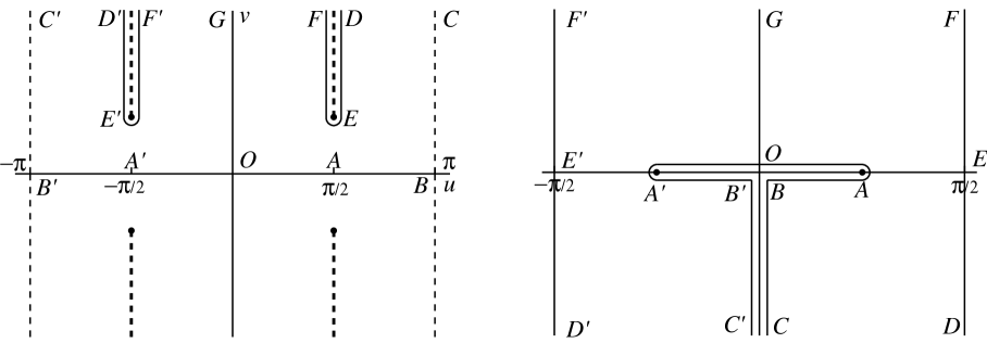
In Figure 3 we show the conformal mapping by $\omega_{\theta}$ from the strip $-\pi\leq u\leq\pi$. We show the images of a number of lines, where we concentrate on $v\geq 0$. For $v\leq 0$ a similar picture can be given. We observe the following useful facts.

  1. 1.

    The image of the interval $[0,\pi]$ must go around a branch cut because $\omega_{\theta}$ is not single valued on this interval; the image point $A$ is given by $A=\arcsin\frac{1}{\sqrt{2}}$.

  2. 2.

    The points $D$ and $F$ are on different sides of the branch cut; the loop $DEF$ around the branch cut is mapped to the vertical $DEF,$ and the same goes for the three points $D^{\prime}E^{\prime}F^{\prime}$.

  3. 3.

    On the positive imaginary axis $u=0,v\geq 0$ $\omega_{\theta}$ has the form (cf. (25))

    $$\omega_{\theta}=i{\rm arcsinh}\frac{\sinh v}{\sqrt{2}}=i\ln\left(\frac{\sinh v}{\sqrt{2}}+\sqrt{\frac{\sinh^{2}v}{2}+1}\right),\quad v\geq 0.$$ (26)
  4. 4.

    On the half-lines $u=\pm\pi,v\geq 0,\;\omega_{\theta}$ has the form

    $$\omega_{\theta}=-i{\rm arcsinh}\frac{\sinh v}{\sqrt{2}}=-i\ln\left(\frac{\sinh v}{\sqrt{2}}+\sqrt{\frac{\sinh^{2}v}{2}+1}\right),\quad v\geq 0.$$ (27)
  5. 5.

    For $\theta$ on the vertical $ED^{\prime}$ we can write $\omega_{\theta}$ in the form

    $$\omega_{\theta}=\frac{1}{2}\pi+i\ln\left(\frac{\cosh v}{\sqrt{2}}+\sqrt{\frac{\cosh^{2}v}{2}-1}\right),\quad\cosh v\geq\sqrt{2}.$$ (28)
  6. 6.

    For $\theta$ on $ED$ we must choose the negative square root, which gives

    $$\omega_{\theta}=\frac{1}{2}\pi-i\ln\left(\frac{\cosh v}{\sqrt{2}}+\sqrt{\frac{\cosh^{2}v}{2}-1}\right),\quad\cosh v\geq\sqrt{2}.$$ (29)

We will also need the following lemma, in order to bound $\omega_{\theta}$ as the imaginary part of $\theta$ tends to $+\infty,$ and hence guarantee that these integrals will converge.

Lemma 1.

If $\theta=u+iv,v>0$, then, as $v\rightarrow+\infty$

$$e^{-i\omega_{\theta}t}=\begin{cases}\mathcal{O}(e^{+vt}),&|u|<\frac{1}{2}\pi,\\ \mathcal{O}(e^{-vt}),&\frac{1}{2}\pi<|u|\leq\pi.\end{cases}$$ (30)
Proof.

Since $\omega_{\theta}=\arcsin\left(\frac{\sin\theta}{\sqrt{2}}\right)$ we have $\sin\omega_{\theta}=\sin\theta/\sqrt{2}$; so

$$e^{-i\omega_{\theta}}=\cos\omega_{\theta}-i\frac{\sin\theta}{\sqrt{2}}.$$ (31)

Hence

$$e^{-i\omega_{\theta}}=\pm\sqrt{1-\frac{\sin^{2}\theta}{{2}}}-i\frac{\sin\theta}{\sqrt{2}}$$ (32)

where the $\pm$ sign in front of the first term has yet to be determined. For small values of $\theta$, it is obvious that we should select the $+$ sign, because both sides of equation (32) have to approach unity as $\theta\to 0$. In fact, the $+$ sign should be chosen throughout the strip $|u|<\frac{1}{2}\pi$. This is because

$$1-\frac{\sin^{2}\theta}{2}=\frac{3+\cos 2\theta}{4}\sim\frac{1}{8}e^{-2i\theta}$$ (33)

as $\theta\to+i\infty$, we conclude that in the strip $|u|<\frac{1}{2}\pi$

$$e^{-i\omega_{\theta}}\sim\frac{1}{2\sqrt{2}}e^{-i\theta}-i\frac{\sin\theta}{\sqrt{2}}\sim\frac{1}{\sqrt{2}}e^{-i\theta}={{\cal O}}(e^{v}),$$ (34)

as $v\to+\infty$. Observe that this is in agreement with the behaviour of $\omega_{\theta}$ on the positive imaginary axis, as given in equation (26). It also agrees with the conformal mapping shown in Figure 3, where we see that the domain $AEFGF^{\prime}E^{\prime}A^{\prime}OA$ is mapped to $\Im\omega_{\theta}>0$. The figure also shows that the domains $ABCDEA$ and $A^{\prime}B^{\prime}C^{\prime}D^{\prime}E^{\prime}A^{\prime}$ are mapped to $\Im\omega_{\theta}<0$. This corresponds to choosing the negative values for $\theta$ in (32) in these domains; this gives the estimate in the second line of (30). This proves the lemma. ∎

Now that we have established the behaviour of the phase function $\omega_{\theta},$ we can proceed to choose an appropriate contour of integration.

2.2 Saddle-point analysis

We will now obtain an asymptotic approximation for $\psi_{R}$ in the exponentially small range outside the main peaks. To find convenient locations for the contours of integration with respect to the stationary points, we will begin with the integral in (22) of Theorem 3 for $\psi_{R}(2-n,t)$, and use the symmetry rule for $\psi_{R}(n,t)$ (cf. Theorem 2) to obtain the result for $\psi_{R}(n,t)$. So, our starting point is

$$\psi_{R}(n,t)=(-1)^{n+1}\psi_{R}(2-n,t)=\frac{(-1)^{n+1}}{2\pi}\int_{-\pi}^{\pi}\frac{e^{-i\theta}}{\sqrt{1+\cos^{2}\theta}}e^{-i(\omega_{\theta}-\theta\alpha)t}\;d\theta,$$ (35)

where $\alpha=n/t$. We have dropped the factor $\frac{1+(-1)^{n+t}}{2}$, because we always can assume that $n$ and $t$ have the same parity; the wavefunction is identically zero otherwise as the walker must always move at each time-step.


We first locate the stationary points or saddle-points in the traditional way, that is, we solve the equation

$$\alpha=\frac{d\omega_{\theta}}{d\theta}=\frac{(\cos\theta_{\alpha})/\sqrt{2}}{\sqrt{1-\sin^{2}\theta_{\alpha}/2}}=\frac{1}{\sqrt{1+\cos^{2}\theta_{\alpha}}}\cos\theta_{\alpha}.$$ (36)

Note that in (36) $\cos\theta_{\alpha}$ and $\alpha$ have the same sign (and $\alpha$ is positive). This gives

$$\cos\theta_{\alpha}=\pm\frac{\alpha}{\sqrt{1-\alpha^{2}}}.$$ (37)

Thus, when $\alpha<1/\sqrt{2},$ this gives two real stationary points

$$\theta_{\alpha}=\pm\arccos\left(\frac{\alpha}{\sqrt{1-\alpha^{2}}}\right),$$ (38)

which are used in the stationary phase method in [29]. If $1/\sqrt{2}<\alpha<1$ these points are purely imaginary, and they are given by

$$\theta_{\alpha}=\pm i\mbox{arccosh}\left(\frac{\alpha}{\sqrt{1-\alpha^{2}}}\right).$$ (39)

When $1/\sqrt{2}<|\alpha|<1$ we shift the contour in the integral representation of the $\psi_{R}$ given in (35) off the real axis to the segments shown in Figure 5. Our modified stationary phase method is in fact a version of the method of steepest descents.

Refer to caption
Figure 4: The saddle-point contour for the integral in (35) for the oscillatory range $0<\alpha<1/\sqrt{2}.$ The interval $[-\pi,\pi]$ can be replaced by a path that runs from $-\pi$ to $-\pi+i\infty$; from that point through the saddle-point at the negative real axis to $-i\infty$ and from that point through the saddle-point at the positive real axis to $+\pi+i\infty$ and then to $+\pi.$ Note that the contributions from the vertical half lines cancel each other out. On the contour shown, the imaginary part of the phase function $-i(\omega_{\theta}-\theta\alpha)t$ is constant (equal to $0,$ in fact). The real part tends to $-\infty$ in the valleys at infinity, and has a maximum at the saddlepoints (black dots).
Refer to caption
Figure 5: The saddle-point contour for the integral in (35) for the exponential-decay range, where $1>\alpha>1/\sqrt{2}$ and the countour runs from $-\pi$ to $-\pi+i\infty.$ It continues from that point through the saddle-point at the positive imaginary axis to $+\pi+i\infty$ and from that point to $+\pi$. Again, the contributions from the vertical half-lines cancel each other. On the contour shown, the imaginary part of the phase function $-i(\omega_{\theta}-\theta\alpha)t$ is constant (equal to $0,$ in fact). The real part tends to $-\infty$ in the valleys at infinity, and has a maximum at the saddle-point (black dot on the positive imaginary axis).

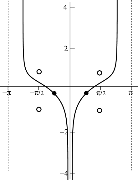
The contour of integration goes through the saddle-point on the positive imaginary axis, that is, through $\theta_{\alpha}=i{\rm arccosh}(\alpha/\sqrt{1-\alpha^{2}})$ and fixes the imaginary part of $i\omega_{\theta}-i\theta\alpha.$ This is equivalent to fixing the real part of $\omega_{\theta}-\theta\alpha.$ We proceed as follows. Consider the integral along the contour in Figure 5. We can make this into a closed contour by adding in segments from $-\pi\to\pi,$ $\pi\to\pi+i\infty$ and $-\pi+i\infty\to-\pi$, thus obtaining an integral over

$$(-\pi,\pi)\cup(\pi,\pi+i\infty)\cup(\pi+i\infty,\theta_{\alpha})\cup(+\theta_{\alpha},-\pi+i\infty)\cup(-\pi+i\infty,-\pi).$$ (40)

The singular points of $\sqrt{1+\cos^{2}\theta}$ follow from solving $\cos^{2}\theta=-1$, which gives $\theta=\pm\pi/2\pm i{\rm arcsinh}(1)$ (see the open dots in Figure 5). We avoid the singularities and branch cuts of the square root in the integrand and of the function $\omega_{\theta}$ (these singularities are the same for both functions; see Figure 3). The integrand is then analytic around and inside the contour in (40), so the integral around the contour is zero. The integrals over the curves indicated below are therefore equal,

$$(-\pi,\pi)=-(\pi,\pi+i\infty)\cup(\pi+i\infty,\theta_{\alpha})\cup(+\theta_{\alpha},-\pi+i\infty)\cup(-\pi+i\infty,-\pi).$$ (41)

The steepest-descent curves for this integral are shown in Figure 5. Furthermore the periodicity of the integrand modulo $2\pi$ means that the segment integrals from $\pi$ to $\pi+i\infty$ and from $-\pi+i\infty$ to $-\pi$ cancel, so these are not shown in Figure 5. Thus, the integral from $-\pi$ to $\pi$ equals the integral along the contour from $-\pi+i\infty$ to $\pi+i\infty$ through $\theta_{\alpha}.$ From Lemma 1 we conclude that

$$e^{-i(\omega_{\theta}-\alpha)t}={{\cal O}}\left(e^{-(1-\alpha)vt}\right)$$ (42)

as $v\to+\infty$ in the strips $-\pi\leq u<-\frac{1}{2}\pi$ and $\frac{1}{2}\pi<u\leq\pi$. Hence, convergence at infinity on a contour as shown in Figure 5 is guaranteed.

2.3 Evaluating the main contribution

We evaluate $e^{-i\omega_{\alpha}+i\theta_{\alpha}\alpha}$ for the saddle-point on the positive imaginary axis, that is, for

$$\theta_{\alpha}=i{\rm arccosh}\left(\frac{\alpha}{\sqrt{1-\alpha^{2}}}\right).$$ (43)

Now, with $x=\alpha/\sqrt{1-\alpha^{2}}$, we obtain

$$\theta_{\alpha}=i{\rm arccosh}\;x=i\ln(x+(x^{2}-1)^{1/2})=i\ln\left(\frac{\alpha+\sqrt{2\alpha^{2}-1}}{\sqrt{1-\alpha^{2}}}\right).$$ (44)

Thus

$$e^{i\theta_{\alpha}\alpha}=\exp\left(-\alpha\ln\left(\frac{\alpha+\sqrt{2\alpha^{2}-1}}{\sqrt{1-\alpha^{2}}}\right)\right)=\left(\frac{\sqrt{1-\alpha^{2}}}{\alpha+\sqrt{2\alpha^{2}-1}}\right)^{\alpha}.$$ (45)

Let us now consider $\omega_{\alpha}=\arcsin\left(\frac{\sin\theta_{\alpha}}{\sqrt{2}}\right)$. We have

$$\cos\theta_{\alpha}=\frac{\alpha}{\sqrt{1-\alpha^{2}}},$$ (46)

so therefore

$$\sin\theta_{\alpha}=\sqrt{1-\alpha^{2}/(1-\alpha^{2})}=\sqrt{\frac{1-2\alpha^{2}}{1-\alpha^{2}}}=i\sqrt{\frac{2\alpha^{2}-1}{1-\alpha^{2}}}.$$ (47)

Thus we obtain

$$\omega_{\alpha}=i{\rm arcsinh}\left(\frac{1}{\sqrt{2}}\sqrt{\frac{2\alpha^{2}-1}{1-\alpha^{2}}}\right).$$ (48)

Now ${\rm arcsinh}\,x=\ln(x+\sqrt{x^{2}+1})$, so

$\displaystyle\omega_{\alpha}$ $\displaystyle=i\ln\left(\frac{\sqrt{2\alpha^{2}-1}}{\sqrt{2}\sqrt{1-\alpha^{2}}}+\left(\frac{2\alpha^{2}-1}{2(1-\alpha^{2})}+1\right)^{1/2}\right)$
$\displaystyle=i\ln\left(\frac{\sqrt{2\alpha^{2}-1}}{\sqrt{2}\sqrt{1-\alpha^{2}}}+\frac{(2\alpha^{2}-1+2-2\alpha^{2})^{1/2}}{\sqrt{2(1-\alpha^{2})}}\right)$
$\displaystyle=i\ln\left(\frac{1+\sqrt{2\alpha^{2}-1}}{\sqrt{2}\sqrt{1-\alpha^{2}}}\right).$ (49)

Thus

$$e^{-i\omega_{\alpha}}=\exp\left(\ln\frac{1+\sqrt{2\alpha^{2}-1}}{\sqrt{2}\sqrt{1-\alpha^{2}}}\right)=\frac{1+\sqrt{2\alpha^{2}-1}}{\sqrt{2}\sqrt{1-\alpha^{2}}}.$$ (50)

and hence

$$e^{-i\omega_{\alpha}+i\theta_{\alpha}\alpha}=\left(\frac{\sqrt{1-\alpha^{2}}}{\alpha+\sqrt{2\alpha^{2}-1}}\right)^{\alpha}\frac{1+\sqrt{2\alpha^{2}-1}}{\sqrt{2}\sqrt{1-\alpha^{2}}}.$$ (51)

Since $\omega_{\theta}-\theta_{\alpha}\alpha$ is an odd function of $\theta_{\alpha}$, we will obtain the reciprocal of this result for the saddle-point $-i\theta_{\alpha}.$ The saddle-point on the positive imaginary axis (when $\alpha>1/\sqrt{2}$) is indeed the relevant one as we will see. The exact saddle-point contours are shown in Figures 4 and 5.


Now that we have established these preliminary results, we can proceed to prove

Theorem 4.

If $1/\sqrt{2}+\varepsilon<|\alpha|<1-\varepsilon,$ then

$$\psi_{R}(n,t)\sim\frac{(-1)^{n+1}\left(\alpha+\sqrt{2\alpha^{2}-1}\right)t^{-1/2}}{\sqrt{2\pi(1-\alpha^{2})\sqrt{2\alpha^{2}-1}}}\left(\left(\frac{\sqrt{1-\alpha^{2}}}{\alpha+\sqrt{2\alpha^{2}-1}}\right)^{\alpha}\frac{1+\sqrt{2\alpha^{2}-1}}{2\sqrt{1-\alpha^{2}}}\right)^{t}.$$ (52)
$$\psi_{L}(n,t)\sim\frac{(-1)^{n}(1-\alpha)t^{-1/2}}{\sqrt{2\pi(1-\alpha^{2})\sqrt{2\alpha^{2}-1}}}\left(\left(\frac{\sqrt{1-\alpha^{2}}}{\alpha+\sqrt{2\alpha^{2}-1}}\right)^{\alpha}\frac{1+\sqrt{2\alpha^{2}-1}}{2\sqrt{1-\alpha^{2}}}\right)^{t}.$$ (53)
Proof.

We prove the equation for $\psi_{R},$ the proof of the equation for $\psi_{L}$ is very similar. Since $\omega_{\theta}=\arcsin\left(\frac{\sin\theta}{\sqrt{2}}\right),$ we have

$$\omega_{\theta}^{\prime\prime}=-\frac{\sin\theta}{\left(1+\cos^{2}\theta\right)^{3/2}}=-i(1-\alpha^{2})\sqrt{2\alpha^{2}-1}.$$ (54)

Since we know that $\cos^{2}\theta_{\alpha}=\alpha^{2}/(1-\alpha^{2}),$ we will obtain

$$1+\cos^{2}\theta_{\alpha}=1/(1-\alpha^{2}),$$ (55)

and we already have (see equation (44))

$$e^{i\theta_{\alpha}}=\frac{\sqrt{1-\alpha^{2}}}{\alpha+\sqrt{2\alpha^{2}-1}}.$$ (56)

The standard formula from steepest descents tells us that

$$\psi_{R}(n,t)\sim\frac{(-1)^{n+1}}{2\pi}\frac{e^{-i\theta_{\alpha}-i(\omega_{\alpha}-\theta_{\alpha}\alpha)t}}{\sqrt{1+\cos^{2}\theta_{\alpha}}}\sqrt{\frac{2\pi}{t|\omega_{\alpha}^{{}^{\prime\prime}}|}}.$$ (57)

The theorem then follows by using equations (50), (53), (55) and (56). ∎


Remark: The wave-mechanics calculation is conceptually much simpler than the path-integral analysis in Carteret et al. [10]. It is also simpler than the calculations of Chen and Ismail [12].

3 Equivalence of the two approaches

We have now completed the calculation begun in [10] and obtained uniformly convergent asymptotics for the wavefunction via both methods. However, the functions $\psi_{L}$ and $\psi_{R}$ derived by each route did not appear to be the same. If they really were different, this would be very alarming, as it would imply either that there is something wrong with Feynman’s equivalence argument in [15] or, more likely, that there was something wrong with our calculation!


The first thing to note is that the quantity raised to the power $t$ in equation (52) dominates the asymptotics of the logarithm of the functions $\psi_{\rm{L}}$ and $\psi_{\rm{R}}$ from the Schrödinger representation. Let us call it $\tilde{B}(\alpha);$ that is,

$$\tilde{B}(\alpha)=\left(\frac{\sqrt{1-\alpha^{2}}}{\alpha+\sqrt{2\alpha^{2}-1}}\right)^{\alpha}\frac{1+\sqrt{2\alpha^{2}-1}}{\sqrt{2}\sqrt{1-\alpha^{2}}}.$$ (58)

These estimates agree with the asymptotics obtained using the method of Saff and Varga [31] as used in [10], although this is not yet apparent. According to the calculation in [10], the corresponding quantity from the path-integral representation, namely $B(\alpha),$ should be

$$2^{-\frac{\alpha}{2}}\times\left(\frac{1+2\alpha-\sqrt{2\alpha^{2}-1}}{1+\alpha}\right)^{\alpha}\left(\frac{\alpha^{2}+\sqrt{2\alpha^{2}-1}}{1-\alpha^{2}}\right)^{(1-\alpha)/2},$$ (59)

which would seem to be a different function.

The demonstration of the equivalence to the result obtained by Saff and Varga’s method needs some identities, starting with

$$\left(1+\sqrt{2\alpha^{2}-1}\right)^{2}=2\left(\alpha^{2}+\sqrt{2\alpha^{2}-1}\right).$$ (60)

Combining $1+2\alpha-\sqrt{2\alpha^{2}-1}$ with the other quantities is rather fiddly (see below). To show that the two solutions (58) and (59) are equivalent, we will now employ the identity

$$\frac{1+2\alpha-\sqrt{2\alpha^{2}-1}}{1+\alpha}=\frac{1+\sqrt{2\alpha^{2}-1}}{\alpha+\sqrt{2\alpha^{2}-1}},$$ (61)

which can easily be verified by cross-multiplication. It follows immediately from this identity that

$$\left(\frac{1+2\alpha-\sqrt{2\alpha-1}}{1+\alpha}\right)^{\alpha}=\left(\frac{1+\sqrt{2\alpha^{2}-1}}{\alpha+\sqrt{2\alpha^{2}-1}}\right)^{\alpha}$$ (62)

and from equation (60) that

$\displaystyle\left(\frac{1-\alpha^{2}}{\alpha^{2}+\sqrt{2\alpha^{2}-1}}\right)^{\frac{\alpha^{2}-1}{2}}$ $\displaystyle=\left(\frac{2(1-\alpha^{2})}{(1+\sqrt{2\alpha^{2}-1})^{2}}\right)^{\frac{\alpha-1}{2}}$ (63)
$\displaystyle=\left(\frac{\sqrt{2}\sqrt{1-\alpha^{2}}}{1+\sqrt{2\alpha^{2}-1}}\right)^{\alpha}\frac{1+\sqrt{2\alpha^{2}-1}}{\sqrt{2}\sqrt{1-\alpha^{2}}}.$ (64)

Thus

$$\left(\frac{1+2\alpha-\sqrt{2\alpha^{2}-1}}{1+\alpha}\right)^{\alpha}\left(\frac{1-\alpha^{2}}{\alpha^{2}-\sqrt{2\alpha^{2}-1}}\right)^{\frac{\alpha-1}{2}}\\ =2^{\alpha/2}\left(\frac{\sqrt{1-\alpha^{2}}}{\alpha+\sqrt{2\alpha^{2}-1}}\right)^{\alpha}\frac{1+\sqrt{2\alpha^{2}-1}}{\sqrt{2}\sqrt{1-\alpha^{2}}}$$ (65)

so that the formulæ  for $\tilde{B}(\alpha)$ and $B(\alpha),$ in (58) and (59) respectively are indeed equivalent.


In fact, the representations for the two functions are completely equivalent, but some of the steps required to prove this need some rather subtle calculations involving special functions, as we will now demonstrate. These technical lemmas will also allow us to rederive the symmetry relations in the wave-mechanics picture that were first proved (for the path-integral picture) in [5]. For convenience we recall the integral representations of Theorem 3

$$\psi_{L}(n,t)=\frac{1}{2\pi}\int_{-\pi}^{\pi}\left(1+\frac{\cos\theta}{\sqrt{1+\cos^{2}\theta}}\right)e^{-i(\omega_{\theta}+\theta\alpha)t}\;d\theta,$$ (66)
$$\psi_{R}(n,t)=\frac{1}{2\pi}\int_{-\pi}^{\pi}\frac{e^{i\theta}}{\sqrt{1+\cos^{2}\theta}}e^{-i(\omega_{\theta}+\theta\alpha)t}\;d\theta.$$ (67)

where $\alpha=n/t$. Note that we have omitted the factors $\frac{1+(-1)^{n+t}}{2}$ since $n$ and $t$ must have the same parity because the walker must move at each time-step.

From these integral representations obtained in the Schrödinger picture [29], we prove in this section the symmetry relations for $\psi_{L}$ and $\psi_{R}$ and the relations first proved for the Jacobi polynomials. These results could previously only be proved in the path-integral picture [5].

3.1 Symmetry properties

Lemma 2.

The function $\psi_{R}$ of (67) satisfies the symmetry relation

$$\psi_{R}(-n,t)=(-1)^{n+1}\psi_{R}(n+2,t).$$ (68)

This is the symmetry relation in Theorem 2 for $\psi_{R}(n,t).$

Proof.

We have, from equation (67)

$$\psi_{R}(n,t)=\frac{1}{\pi}\int_{0}^{\pi}\frac{\cos((n-1)\theta)\cos(\omega_{\theta}t)}{\sqrt{1+\cos^{2}\theta}}\,d\theta-\frac{1}{\pi}\int_{0}^{\pi}\frac{\sin((n-1)\theta)\sin(\omega_{\theta}t)}{\sqrt{1+\cos^{2}\theta}}\,d\theta.$$ (69)

The first integral vanishes when $n$ is even, the second one when $n$ is odd. To verify this, split $[0,\pi]=[0,\frac{1}{2}\pi]\cup[\frac{1}{2}\pi,\pi]$ and write on the second interval $\theta=\pi-\theta^{\prime}$. We conclude that $\psi_{R}(1-n,t)=\psi_{R}(1+n,t)$ when $n$ is odd, and $\psi_{R}(1-n,t)=-\psi_{R}(1+n,t)$ when $n$ is even. This proves the lemma. ∎

Lemma 3.

The function $\psi_{L}$ of equation (66) satisfies the symmetry relation

$$(t-n)\psi_{L}(-n,t)=(-1)^{n}(t+n)\psi_{L}(n,t).$$ (70)

This is the symmetry relation in Theorem 2 for $\psi_{L}(n,t).$

Proof.

We have from (66)

$$\psi_{L}(n,t)=\widetilde{\psi}_{L}(n,t)+\frac{1}{2\pi}\int_{-\pi}^{\pi}\frac{\cos\theta}{\sqrt{1+\cos^{2}\theta}}e^{-i(t\omega_{\theta}+n\theta)}\,d\theta,$$ (71)

where

$\displaystyle\widetilde{\psi}_{L}(n,t)$ $\displaystyle=\frac{1}{2\pi}\int_{-\pi}^{\pi}e^{-i(t\omega_{\theta}+n\theta)}\,d\theta$ (72)
$\displaystyle=\frac{1}{\pi}\int_{0}^{\pi}\cos(n\theta)\cos(t\omega_{\theta})\;d\theta-\frac{1}{\pi}\int_{0}^{\pi}\sin(n\theta)\sin(t\omega_{\theta})\,d\theta.$ (73)

The first integral vanishes when $n$ is odd, the second one when $n$ is even. This gives the symmetry relation

$$\widetilde{\psi}_{L}(-n,t)=(-1)^{n}\widetilde{\psi}_{L}(n,t).$$ (74)

Next observe that

$$\frac{d\omega_{\theta}}{d\theta}=\frac{\cos\theta}{\sqrt{1+\cos^{2}\theta}},$$ (75)

and that an integration by parts in the integral in equation (71) gives us that

$$\psi_{L}(n,t)=\frac{t-n}{t}\widetilde{\psi}_{L}(n,t).$$ (76)

Finally we use equations (74) and (76) to complete the proof of the lemma. ∎

Remark: The symmetry relations for $\psi_{L}$ and $\psi_{R}$ also follow from the following property of the Jacobi polynomials:

$$\binom{m}{\ell}J_{m}^{(u,-\ell)}(x)=\binom{m+u}{\ell}\left(\frac{1+x}{2}\right)^{\ell}J_{m-\ell}^{(u,\ell)}(x),\quad 0\leq\ell\leq m.$$ (77)

This formula follows from the representation of the Jacobi polynomial in terms of the hypergeometric function (cf. [34, p. 151, (6.35)]) in combination with a functional relation of this function (third line of equation (5.5) in [34, p. 110]). The result in (77) combines the first case in (10) with the second case, and it also implies the symmetry rule for $\psi_{R},$ and similarly for (11).

3.2 The ${\boldsymbol{\psi}-}$functions in terms of Jacobi polynomials

We will now prove that the $\psi-$functions with the integral representations given in (66) and (67) can be written in terms of the Jacobi polynomials as in Theorem 2. This step will require the use of generating functions. These provide a method for writing a series as the coefficients of a formal power series, in a dummy variable, $z,$ for ease of manipulation. The powers of $z$ are then the summation variable for the series. For a basic introduction to the theory of generating functions, see [36]; for an advanced treatment, see [19].

We will use these generating functions to give us an exact representation of the $\Psi$ functions as functions of $t,$ thus each labelled term in the series will be the function for that value of $t.$ Therefore, our approach will be based on generating functions that contain the $\psi-$functions with $t$ as the summation variable. We only consider sums of $\psi-$functions with $n$ and $t$ having the same parity.

3.3 Some generating functions for ${\boldsymbol{\psi}}$

For convenience, we will define the following generating functions, which can be obtained from the Schrödinger representation of the wavefunction.

Theorem 5.

Consider the generating functions for $|z|<1$:

$\displaystyle F_{m}(z)$ $\displaystyle=\sum_{t=0}^{\infty}\psi_{R}(2m+1,2t+1)z^{t},$ (78)
$\displaystyle G_{m}(z)$ $\displaystyle=\sum_{t=0}^{\infty}\psi_{R}(2m,2t)z^{t},$ (79)
$\displaystyle H_{m}(z)$ $\displaystyle=\sum_{t=0}^{\infty}\widetilde{\psi}_{L}(2m+1,2t+1)z^{t},$ (80)
$\displaystyle I_{m}(z)$ $\displaystyle=\sum_{t=0}^{\infty}\widetilde{\psi}_{L}(2m,2t)z^{t},$ (81)

where $\widetilde{\psi}_{L}(n,t)$ is defined in (72). After the summations have been performed these functions become, respectively,

$\displaystyle F_{m}(z)$ $\displaystyle=\frac{2^{m-\frac{1}{2}}z^{m}}{\sqrt{1+z^{2}}(1-z+\sqrt{1+z^{2}})^{2m}},$ $\displaystyle m=0,1,2,\ldots,$ (82)
$\displaystyle G_{m}(z)$ $\displaystyle=-\frac{2^{m-1}z^{m}}{\sqrt{1+z^{2}}(1-z+\sqrt{1+z^{2}})^{2m-1}},$ $\displaystyle m=1,2,3\ldots,$ (83)
$\displaystyle G_{0}(z)$ $\displaystyle=\frac{z}{\sqrt{1+z^{2}}(1-z+\sqrt{1+z^{2}})},$ (84)
$\displaystyle H_{m}(z)$ $\displaystyle=\frac{2^{m-\frac{1}{2}}(1+z)z^{m}}{\sqrt{1+z^{2}}(1-z+\sqrt{1+z^{2}})^{2m+1}},$ $\displaystyle m=0,1,2,\ldots$ (85)
$\displaystyle I_{m}(z)$ $\displaystyle=\frac{2^{m-1}(1+z)z^{m}}{\sqrt{1+z^{2}}(1-z+\sqrt{1+z^{2}})^{2m}},$ $\displaystyle m=1,2,3\ldots,$ (86)
$\displaystyle I_{0}(z)$ $\displaystyle=\frac{1}{\sqrt{1+z^{2}}}-\frac{z}{\sqrt{1+z^{2}}(1-z+\sqrt{1+z^{2}})}.$ (87)

These summations can be done using some fiddly, but essentially mechanical manipulations; we have included detailed proofs for $F_{m}(z)$ and a sketch of that for $G_{m}(z)$ in an appendix, in Subsection 6.1. The other generating functions can be obtained via similar constructions.


For $H_{m}(z)$ we obtain

$\displaystyle H_{m}(z)$ $\displaystyle=\frac{1}{2\pi}\int_{-\pi}^{\pi}{e^{-i((2m+1)\theta+\omega_{\theta})}}\,\frac{1}{1-ze^{-2i\omega_{\theta}}}\,d\theta$ (88)
$\displaystyle=\frac{1+z}{2\pi\sqrt{2}}\int_{0}^{\pi}\frac{\cos((2m+2)\theta)-\cos(2m\theta)}{1-2z\cos 2\omega_{\theta}+z^{2}}\,d\theta$ (89)
$\displaystyle=\frac{1+z}{2(1-z)}\left[F_{m+1}(z)-F_{m}(z)\right].$ (90)

Taken together with (82), this becomes equation (85).


For $I_{m}(z)$ we have a useful intermediate result, namely that

$$I_{m}(z)=\frac{\sqrt{2}}{4(1-z)}\left[2(2-z)F_{m}(z)-zF_{|m-1|}(z)-zF_{m+1}(z)\right].$$ (91)

It remains to compare these with some generating functions for Jacobi polynomials. For an introduction to the theory of Jacobi polynomials we refer the reader to [30, 7] and [34]. This correspondence between the two sets of generating functions forms the central plank of the Feynman equivalence between the two representations of the wave-function for this system.

3.4 Comparing the generating functions for $\boldsymbol{\psi}$

We now compare the generating functions (82) – (87) from the wave-mechanics representation, with the generating function of the Jacobi polynomials (cf. [7, p. 298]) from the path-integral representation [10] to complete our proof of the equivalence of the two approaches:

$$\sum_{k=0}^{\infty}J_{k}^{(r,s)}(x)z^{k}=\frac{2^{r+s}}{R(1-z+R)^{r}(1+z+R)^{s}},\quad|z|<1,$$ (92)

where $R=\sqrt{1-2xz+z^{2}}$, which for $x=0$ becomes

$$\sum_{k=0}^{\infty}J_{k}^{(r,s)}(0)z^{k}=\frac{2^{r+s}}{\sqrt{1+z^{2}}(1-z+\sqrt{1+z^{2}})^{r}(1+z+\sqrt{1+z^{2}})^{s}}.$$ (93)

By applying the Cauchy integral formula we find that

$$J_{k}^{(r,s)}(0)=\frac{2^{r+s}}{2\pi i}\oint\frac{dz}{\sqrt{1+z^{2}}(1-z+\sqrt{1+z^{2}})^{r}(1+z+\sqrt{1+z^{2}})^{s}z^{k+1}},$$ (94)

where the integral is taken over a circle with radius less than unity.

Lemma 4.

For $n=0$ we have

$\displaystyle\psi_{R}(0,0)$ $\displaystyle=0,$ (95)
$\displaystyle\psi_{R}(0,2t)$ $\displaystyle=\frac{1}{2}J_{t-1}^{(1,0)}(0)=\frac{1}{2}(-1)^{t-1}J_{t-1}^{(0,1)}(0),\quad t=2,4,6,\ldots\,.$ (96)

For $0<n\leq t$, $n$ and $t$ having the same parity, we have

$$\psi_{R}(n,t)=2^{-\frac{n}{2}}(-1)^{\frac{t-n}{2}}(-1)^{n+1}J_{\frac{t-n}{2}}^{(0,n-1)}(0).$$ (97)

This gives the first case of equation (10) from the wave-mechanics representation, which was originally obtained via the path-integral method.

Proof.

From (78) and (82) we find, as in (94),

$$\psi_{R}(2m+1,2t+1)=\frac{2^{m-\frac{1}{2}}}{2\pi i}\oint\frac{z^{m}}{\sqrt{1+z^{2}}(1-z+\sqrt{1+z^{2}})^{2m}}\,\frac{dz}{z^{t+1}}.$$ (98)

We now compare (94) with (98) and take $u=2m,$ $v=0,$ and $s=t-m.$ This gives

$$\psi_{R}(2m+1,2t+1)=2^{-m-\frac{1}{2}}J_{t-m}^{(2m,0)}(0),\quad 0\leq m\leq t.$$ (99)

Using the symmetry rule for the Jacobi polynomials

$$J_{n}^{(r,s)}(-x)=(-1)^{n}J_{n}^{(s,r)}(x),$$ (100)

which follows from (92) by putting $x\to-x,z\to-z$, we find

$$\psi_{R}(2m+1,2t+1)=2^{-m-\frac{1}{2}}(-1)^{t-m}J_{t-m}^{(0,2m)}(0),\quad 0\leq m\leq t.$$ (101)

For the even case, we obtain from (79), (83), and (100)

$$\psi_{R}(2m,2t)=-2^{-m}J_{t-m}^{(2m-1,0)}(0)=-2^{-m}(-1)^{t-m}J_{t-m}^{(0,2m-1)}(0),\quad 0<m\leq t,$$ (102)

and from (79) and (84) we obtain (95). Combining (101) and (102) in one formula gives (97). This proves the lemma. ∎

Lemma 5.

For $n=0$ we have

$\displaystyle\psi_{L}(0,0)$ $\displaystyle=1,$ (103)
$\displaystyle\psi_{L}(0,t)$ $\displaystyle=J_{t/2}^{(0,0)}(0)-\frac{1}{2}J_{t/2-1}^{(1,0)}(0),\quad t=2,4,6,\ldots\,.$ (104)

For $0<n<t$, $n$ and $t$ having the same parity, we have

$$\psi_{L}(n,t)=2^{-n/2-1}(-1)^{(t-n)/2-1}J_{(t-n)/2-1}^{(1,n)}(0).$$ (105)

This gives the first case of (11) from the path-integral representation, now obtained via wave-mechanics.


Proof.

We obtain from (80) and (85)

$\displaystyle\widetilde{\psi}_{L}(2m+1,2t+1)$ $\displaystyle=2^{-m-\frac{3}{2}}\left[J_{t-m}^{(2m+1,0)}(0)+J_{t-m-1}^{(2m+1,0)}(0)\right]$ (106)
$\displaystyle=2^{-m-\frac{3}{2}}\frac{2t+1}{t+m+1}J_{t-m}^{(2m+1,-1)}(0),$ (107)

where we have used the relation for the Jacobi polynomials (cf. [1, p.782, (22.7.19)])

$$(u+v+2k)J_{k}^{(u,v-1)}(x)=(u+v+k)J_{k}^{(u,v)}(x)+(u+k)J_{k-1}^{(u,v)}(x).$$ (108)

We use (77), (76) and (100), and obtain

$$\psi_{L}(2m+1,2t+1)=2^{-m-\frac{3}{2}}(-1)^{t-m-1}J_{t-m-1}^{(1,2m+1)}(0).$$ (109)

For the even case we obtain from (81) and (86)

$\displaystyle\widetilde{\psi}_{L}(2m,2t)$ $\displaystyle=2^{-m-1}\left[J_{t-m}^{(2m,0)}(0)+J_{t-m-1}^{(2m,0)}(0)\right]$ (110)
$\displaystyle=2^{-m-1}(-1)^{t-m-1}\frac{t}{t-m}J_{t-m-1}^{(1,2m)}(0),$ (111)

where we used (108), (77) and (100). By using (76) we obtain

$$\psi_{L}(2m,2t)=2^{-m-1}(-1)^{t-m-1}J_{t-m-1}^{(1,2m)}(0),\quad m=1,2,3,\ldots\,.$$ (112)

From (81) and (87) we obtain (103). Combining (109) and (112) into a single formula gives equation (105). This proves the lemma. ∎

As we have now established that both sets of generating functions match, this completes the proof of the equivalence of the results obtained via the path-integral and wave-mechanics representations. It should be noted that we have proved the two representations are exactly equivalent for all time, as opposed to being only asymptotically equivalent in the long-time limit. It is one of the curious features of generating function methods that they can be used to prove the existence of a one-to-one correspondence between the two sets (i.e., our $\psi$-functions) counted by the two series, without actually finding the explicit bijection.

3.5 Summary of the equivalence results

While the coined quantum walk can be thought of as a quantum analogue of the discrete-time classical random walk [35, 2], it should be noted that the quantum model inherits its discrete time parameter directly from the classical model; the discreteness was not introduced by hand as part of the quantization procedure. Also, we have not defined a Hamiltonian for this system at all, so the problem of ambiguities in the time derivatives of the action does not arise. We have now shown the full Feynman equivalence for this system, though some results seem easier to derive in one approach than in the other.

  • We have obtained the symmetry rules directly from the integral representations for the $\psi$-functions. It is not necessary to represent the $\psi$-functions as Jacobi poynomials and then use the symmetry properties of Jacobi polynomials (as was done in [5]) to obtain this result.

  • The relations between the $\psi$-functions and the Jacobi polynomials have been obtained directly from the integral representations, though we needed to develop some technical tools for this. These consisted of a few extra properties of the Jacobi polynomials, and the generating functions containing the $\psi$-functions. The proofs using these generating functions are conceptually straightforward, although the details are quite technical. The Feynman path-integral approach of [5] (which is a finite sum here) would seem to be simpler if these relations are all one wants.

  • We were able to establish some new expressions for the values of the two components of the $\psi$-function at $n=0$ as a function of time, in equations (95) and (103), which were not known before.

4 Physical interpretation of these results

Now that we have established that the rather counter-intuitive results obtained from the wave-mechanics picture really are equivalent to the Airy functions obtained from the path-integral approach, we are left with the little mystery of their physical interpretation. In this region of exponential decay these waves have complex wavenumbers. This phenomenon is called evanescence. And herein lies the mystery; the conventional wisdom is that evanescent waves are only ever seen in the presence of absorbing media, such as light waves being absorbed into a conducting surface, but there is no such surface here and the evolution is unitary, by the initial assumptions that went into constructing the model. In fact, the phenomenon of evanescence is rather more widespread; it occurs in a great many systems if you know where to look. In a pioneering paper in the early 1990s, Michael Berry showed that evanescent behaviour is much more common than had been previously thought, after being inspired by some work by Aharonov, Anandan, Popescu and Vaidman in [3]. Berry gave a detailed discussion of how this phenomenon occurs in optics, at the edges of the almost ubiquitous “Gaussian” beams in [9].

The wavefunction for this system tends to an Airy function in the asymptotic limit, as was proved analytically in [10]. We evaluated the integrals in the path-integral picture using the method of steepest descents, which in this case featured a pair of coalescing saddle-points [10, 27]. Since then, various authors have discussed the connection between the discrete walk on the infinite line and interference phenomena in the quantum optics of dispersive media. This connection was first described by Knight, Roldan and Sipe in a series of papers [25, 24, 26] and further clarified by Kendon and Sanders in [23].

As we enter the exponential decay region, the two original stationary points of the phase function merge and then two new saddle-points are born, which move off the real axis as a complex conjugate pair. The behaviour of the momentum closely follows that of $\omega_{\theta},$ which was plotted in Figure 2. In the wave-mechanics picture, we found that the momentum becomes purely imaginary in the exponential decay region; indeed, the techniques we used to evaluate the integral relied on this fact. So, the behaviour of the walk in the exponential decay region is a pure exponential decay; there is no oscillatory behaviour.

Within the interpretation begun by Knight et al., it was first suggested to us by Achim Kempf [22] that the specific evanescence phenomena that we have discussed in this paper are analogues of what are called the Sommerfeld and Brillouin precursors. Specifically, the exponential decay region can be identified with the Sommerfeld precursor (see for example, [17]) and the distinctive peaks in the probability distribution would be an example of the Brillouin Precursor (see for example [16]). Our results here and the previous results in [10] provide the first analytic evidence for this identification.

5 Conclusions

In this paper we have completed the analysis begun in [10], thus meeting the challenge made in [5] to prove all their theorems about the unrestricted quantum walk on the line in both the path-integral and wave-mechanics representations. We have also proved some additional identities that we believe to be novel. In the course of doing this, we have had to generalise the method of stationary phase in a way that may have applications beyond this problem. We have also proved the exact Feynman equivalence between the two representations directly, by reducing the problem to purely combinatorical constructions which may also be of wider interest.

Lastly, we have supplied a physical interpretation for our results, in terms of certain evanescent phenomena from the quantum optics of dispersive media. This interpretation is a somewhat counter-intuitive one, as it would seem to require an effective dissipation that acts on the walker in a way that is analogous to the effect of a dielectric medium on light, despite the fact that the evolution of the system is unitary by assumption.

Acknowledgments

HAC would like to acknowledge some inspiring conversations with Sir Michael Berry, Mourad Ismail and Achim Kempf. HAC was supported by MITACS, and would like to thank the Perimeter Institute and the IQC at the University of Waterloo for hospitality. LBR would also like to thank Ashwin Nayak for some interesting conversations. The research of LBR was partially supported by an NSERC operating grant. NMT acknowledges financial support from Ministerio de Educación y Ciencia (Programa de Sabáticos) from project SAB2003-0113.

References

  • [1] Milton Abramowitz and Irene A. Stegun (Eds), Handbook of Mathematical Functions, With Formulas, Graphs, and Mathematical Tables, Dover, June 1974,   ISBN=0486612724.
  • [2] Dorit Aharonov, Andris Ambainis, Julia Kempe, and Umesh Vazirani, Quantum Walks On Graphs, Proceedings of ACM Symposium on Theory of Computation (STOC’01), July 2001, Association for Computing Machinery, New York, 2001, quant-ph/0012090, pp. 50–59.
  • [3] Y. Aharonov, J. Anandan, S. Popescu, and L. Vaidman, Superpositions of Time Evolutions of a Quantum System and a Quantum Time-Translation Machine, Phys. Rev. Lett. 64 (1990), 2965–8.
  • [4] Y. Aharonov, L. Davidovich, and N. Zagury, Quantum random walks, Phys. Rev. A 48 (1993), 1687.
  • [5] A. Ambainis, E. Bach, A. Nayak, A. Vishwanath, and J. Watrous, One-Dimensional Quantum Walks, Proceedings of the 33rd ACM Symposium on Theory of Computation (STOC’01), July 2001, Association for Computing Machinery, New York, 2001, pp. 37–49.
  • [6] Andris Ambainis, Quantum walks and their algorithmic applications, 2004, quant-ph/0403120.
  • [7] G. E. Andrews, R. A. Askey, and R. Roy, Special Functions, Cambridge University Press, 1999,  ISBN=0-521-62321-9.
  • [8] George B. Arfken and Hans-Jurgen Weber, Mathematical Methods for Physicists, 5th ed., Academic Press, 2000,  ISBN=0-12-059825-6.
  • [9] M. V. Berry, Evanescent and real waves in quantum billiards and Gaussian beams, J. Phys. A: Math. Gen. 27 (1994), L391–398.
  • [10] Hilary A. Carteret, Mourad Ismail, and Bruce Richmond, Three routes to the exact asymptotics of the one-dimensional quantum walk, J. Phys. A. 36 (2003), 8775–8795, quant-ph/0303105.
  • [11]  , Three routes to the exact asymptotics of the one-dimensional quantum walk, 2003, quant-ph/0303105. Note that the journal version contains a typo here. Please see the new archive version for the correct equation.
  • [12] L.-D. Chen and M. E. H. Ismail, On Asymptotics of Jacobi Polynomials, SIAM J. Math. Anal. 22 (1991), 1442–1449.
  • [13] Andrew M. Childs, Edward Farhi, and Sam Gutmann, An example of the difference between quantum and classical random walks, Quantum Information Processing 1 (2002), 35–43, quant-ph/0103020.
  • [14] Edward Farhi and Sam Gutmann, Quantum computation and decision trees, Phys. Rev. A 58 (1998), 915–928, quant-ph/9706062.
  • [15] R. P. Feynman and A. R. Hibbs, Quantum Mechanics and Path Integrals, McGraw-Hill, 1965,   ISBN=0-07-020650-3.
  • [16] Richard Fitzpatrick, The Brillouin Precursor, from PHY387K: Graduate course in classical electromagnetism (electromagnetic wave propagation in dielectrics), 2002, The University of Texas at Austin, available online at http://farside.ph.utexas.edu/teaching/jk1/lectures/node67.html.
  • [17]  , The Sommerfeld Precursor, from PHY387K: Graduate course in classical electromagnetism (electromagnetic wave propagation in dielectrics), 2002, The University of Texas at Austin, available online at http://farside.ph.utexas.edu/teaching/jk1/lectures/node64.html.
  • [18] Wolfgang Gawronkski and Bruce Shawyer, Progress in Approximation Theory, ch. Strong Asymptotics and the Limit Distribution of the Zeroes of Jacobi Polynomials $P_{n}^{an+\alpha,bn+\beta},$ ISBN=0-12-516750-4, pp. 379–404, Academic Press, 1991.
  • [19] Ian P. Goulden and David M. Jackson, Combinatorial Enumeration, Dover, 2004,  ISBN=0486435970.
  • [20] I. S. Gradshteyn and I. W. Ryzhik, Table of Integrals, Series and Products, 6th ed., Academic Press, New York, 1996,  ISBN=0122947576.
  • [21] J. Kempe, Quantum random walks – an introductory overview, Contemporary Physics 44 (2003), 307–327, quant-ph/0303081.
  • [22] Achim Kempf, 2004, Private Communication.
  • [23] Viv Kendon and Barry C. Sanders, Complementarity and quantum walks, Physical Review A 71 (2005), 022307, quant-ph/0404043.
  • [24] Peter L. Knight, Eugenio Roldan, and John E. Sipe, Optical Cavity Implementations of the Quantum Walk, Optics Communications 227 (2003), 147–157, quant-ph/0305165.
  • [25]  , Propagating Quantum Walks: the origin of interference structures, J. Mod. Opt. 51 (2003), 1761–1777, quant-ph/0312133.
  • [26]  , Quantum Walk on the line as an interference phenomenon, Physical Review A 68 (2003), 020301, quant-ph/0304201.
  • [27] J. P. McClure and R. Wong, Justification of the stationary phase approximation in time-domain asymptotics, Proc. R. Soc. Lond. A. 453 (1997), 1019–1031.
  • [28] David A. Meyer, From quantum cellular automata to quantum lattice gases, J. Stat. Phys. 85 (1996), 551–574, quant-ph/9604003.
  • [29] Ashwin Nayak and Ashvin Vishwanath, Quantum Walk on the Line, 2000, quant-ph/0010117.
  • [30] Frank W. J. Olver, Asymptotics and Special Functions, AKP Classics, 1997,   ISBN=1-56881-069-5.
  • [31] E. B. Saff and R. S. Varga, The sharpness of Lorentz’s theorem on incomplete polynomials, Transactions of The American Mathematical Society 249 (April 1979), 163–186.
  • [32] H. M. Srivastava and J. P. Singhal, New Generating Functions for Jacobi and Related Polynomials, J. Math. Anal. Appl. 41 (1973), 748–752.
  • [33] Mario Szegedy, Spectra of quantized walks and a $\sqrt{\delta\epsilon}$ rule, 2004, quant-ph/0401053.
  • [34] Nico M. Temme, Special Functions: An Introduction to the Classical Functions of Mathematical Physics, John Wiley & Sons, Inc., 1996,   ISBN=0-471-11313-1.
  • [35] John Watrous, model of the coined quantum walk on the line, 1999?, Unpublished.
  • [36] Herbert S. Wilf, Generatingfunctionology, 2nd ed., Academic Press, 1994,  ISBN=0127519564.

6 Appendices

6.1 Construction of the generating functions

Here we give the details of the construction for the generating functions from Subsection 3.3.

6.1.1 Proof of the construction for $\boldsymbol{F_{m}(z)}$

Proof.

We give a detailed proof for $F_{m}(z)$. We substitute equation (67) into equation (78) and obtain

$$F_{m}(z)=\frac{1}{2\pi}\int_{-\pi}^{\pi}\frac{e^{-i(2m\theta+\omega_{\theta})}}{\sqrt{1+\cos^{2}\theta}}\,\frac{1}{1-ze^{-2i\omega_{\theta}}}\;d\theta\\ =\frac{1}{2\pi}\int_{-\pi}^{\pi}\frac{e^{-i(2m\theta+\omega_{\theta})}}{\sqrt{1+\cos^{2}\theta}}\,\frac{1-z\cos 2\omega_{\theta}-iz\sin 2\omega_{\theta}}{1-2z\cos 2\omega_{\theta}+z^{2}}\;d\theta\\ =\frac{1}{2\pi}\int_{-\pi}^{\pi}\frac{\{\cos(2m\theta+\omega_{\theta})-i\sin(2m\theta+\omega_{\theta})\}\{1-z\cos 2\omega_{\theta}-iz\sin 2\omega_{\theta}\}}{\sqrt{1+\cos^{2}\theta}\,(1-2z\cos 2\omega_{\theta}+z^{2})}\;d\theta.$$ (113)

Since $\omega_{\theta}$ is an odd function, the imaginary parts will vanish. The interval $[-\pi,\pi]$ can be reduced to $[0,\pi]$ and we obtain

$\displaystyle F_{m}(z)$ $\displaystyle=\frac{1}{\pi}\int_{0}^{\pi}\frac{\cos(2m\theta+\omega_{\theta})(1-z\cos 2\omega_{\theta})-z\sin 2\omega_{\theta}\sin(2m\theta+\omega_{\theta})}{\sqrt{1+\cos^{2}\theta}\,(1-2z\cos 2\omega_{\theta}+z^{2})}\;d\theta$ (114)
$\displaystyle=\frac{1}{\pi}\int_{0}^{\pi}\frac{\cos(2m\theta+\omega_{\theta})}{\sqrt{1+\cos^{2}\theta}\,(1-2z\cos 2\omega_{\theta}+z^{2})}\;d\theta$
$\displaystyle\quad\quad-\frac{z}{\pi}\int_{0}^{\pi}\frac{\cos(2m\theta+\omega_{\theta})\cos(2\omega_{\theta})+\sin(2m\theta+\omega_{\theta})\sin 2\omega_{\theta}}{\sqrt{1+\cos^{2}(\theta)}\,(1-2z\cos 2\omega_{\theta}+z^{2})}\;d\theta.$ (115)

The numerator of the second integral can be written as $\cos(2m\theta-\omega_{\theta})$, and it follows that

$\displaystyle F_{m}(z)$ $\displaystyle=\frac{1}{\pi}\int_{0}^{\pi}\frac{\cos(2m\theta+\omega_{\theta})}{\sqrt{1+\cos^{2}\theta}\,(1-2z\cos 2\omega_{\theta}+z^{2})}\;d\theta$
$\displaystyle\quad\quad-\frac{z}{\pi}\int_{0}^{\pi}\frac{\cos(2m\theta-\omega_{\theta})}{\sqrt{1+\cos^{2}\theta}\,(1-2z\cos 2\omega_{\theta}+z^{2})}\;d\theta.$ (116)

We can now use simple trigonometric identities for the cosines in the numerators, to obtain

$\displaystyle F_{m}(z)$ $\displaystyle=\frac{1}{\pi}\int_{0}^{\pi}\frac{\cos 2m\theta\cos\omega_{\theta}-\sin 2m\theta\sin\omega_{\theta}}{\sqrt{1+\cos^{2}\theta}\,(1-2z\cos 2\omega_{\theta}+z^{2})}\,\,d\theta$
$\displaystyle\quad\quad-\frac{z}{\pi}\int_{0}^{\pi}\frac{\cos 2m\theta\cos\omega_{\theta}+\sin 2m\theta\sin\omega_{\theta}}{\sqrt{1+\cos^{2}\theta}\,(1-2z\cos 2\omega_{\theta}+z^{2})}\;d\theta.$ (117)

Now we use $\sin\omega_{\theta}=(\sin\theta)/\sqrt{2}$, and observe that the terms with the sine functions do not contribute to the integrals; this follows easily by performing the transformation $\theta=\theta^{\prime}+\frac{1}{2}\pi$. Using also $\cos\omega_{\theta}=\sqrt{\frac{1}{2}(1+\cos^{2}\theta)}$, we obtain

$$F_{m}(z)=\frac{1-z}{\pi\sqrt{2}}\int_{0}^{\pi}\frac{\cos(2m\theta)}{1-2z\cos 2\omega_{\theta}+z^{2}}\,d\theta.$$ (118)

For the final step we use formula (3.615) (1) of Gradshteyn and Ryzhik [20], that is,

$$\int_{0}^{\frac{1}{2}\pi}\frac{\cos(2m\theta)}{1-a^{2}\sin^{2}\theta}\,d\theta=\frac{(-1)^{m}\pi}{2\sqrt{1-a^{2}}}\frac{(1-\sqrt{1-a^{2}})^{2m}}{a^{2m}},\quad|a^{2}|<1,\quad m=0,1,2,\ldots\;.$$ (119)

We observe that $\cos 2\omega_{\theta}=\cos^{2}\theta$, and take $a^{2}=-2z/(1-z)^{2}$. This gives the expression in (82), as advertised.

6.1.2 Outline of the proof for $\boldsymbol{G_{m}(z)}$

The proof of equation (83) for $G_{m}(z)$ uses essentially the same manipulations:

$\displaystyle G_{m}(z)$ $\displaystyle=\frac{1}{2\pi}\int_{-\pi}^{\pi}\frac{e^{i(1-2m)\theta}}{\sqrt{1+\cos^{2}\theta}}\,\frac{1}{1-ze^{-2i\omega_{\theta}}}\;d\theta$ (120)
$\displaystyle=\frac{1}{2\pi}\int_{-\pi}^{\pi}\frac{\cos(2m-1)\theta(1-z\cos 2\omega_{\theta})-z\sin(2m-1)\theta\,\sin 2\omega_{\theta}}{\sqrt{1+\cos^{2}\theta}\,(1-2z\cos 2\omega_{\theta}+z^{2})}\;d\theta.$ (121)

The second integral can be broken into two terms as follows:

$\displaystyle G_{m}(z)$ $\displaystyle=\frac{1}{\pi}\int_{0}^{\pi}\frac{\cos(2m-1)\theta}{\sqrt{1+\cos^{2}\theta}\,(1-2z\cos 2\omega_{\theta}+z^{2})}\;d\theta$ (122)
$\displaystyle\quad-\frac{z}{\pi}\int_{0}^{\pi}\frac{\cos(2m-1)\theta\cos 2\omega_{\theta}+\sin(2m-1)\theta\sin 2\omega_{\theta}}{\sqrt{1+\cos^{2}\theta}\,(1-2z\cos 2\omega_{\theta}+z^{2})}\;d\theta.$ (123)

The first integral vanishes (substitute $\theta=\theta^{\prime}+\frac{1}{2}\pi$). The same holds for the contributions from the cosine terms in the second integral. This gives

$$G_{m}(z)=-\frac{z}{\pi}\int_{0}^{\pi}\frac{\sin(2m-1)\theta\sin\theta}{1-2z\cos 2\omega_{\theta}+z^{2}}\;d\theta.$$ (124)

Using the fact that

$\displaystyle\cos 2m\theta$ $\displaystyle=\cos(2m-1)\theta\cos\theta+\sin(2m-1)\theta\sin\theta$ (125)
$\displaystyle\cos(2m-2)\theta$ $\displaystyle=\cos(2m-1)\theta\cos\theta-\sin(2m-1)\theta\sin\theta$ (126)

we can then write

$$G_{m}(z)=\frac{z}{2\pi}\int_{0}^{\pi}\frac{\cos 2m\theta-\cos(2m-2)\theta}{1-2z\cos 2\omega_{\theta}+z^{2}}\;d\theta,$$ (127)

and we see (cf. (118)) that we can express $G_{m}(z)$ in terms of two $F_{m}(z)$ functions. This gives equation (83). ∎

6.2 Lagrange inversion asymptotics

Suppose we have an unknown function $w$ that we assume can be written as an (as yet unknown) power series. All we know about this power series is that it can be written as a recursion relation

$\displaystyle w=z\varphi(w),$ $\displaystyle\varphi(0)\neq 0,$ (128)

where $\varphi(w)$ is some generating function that is defined as an implicit function of $z$. We would like to find $w$ as an explicit function of $z,$ so we can express some other function $f(w)$ as an explicit power series in $z.$ Lagrange Inversion enables us to do this, and tells us that we can write

$$f(w)=\sum_{n\geq 1}\frac{t^{n}}{n}[\lambda^{n-1}]f^{{}^{\prime}}(\lambda)\phi^{n}(\lambda),$$ (129)

where $\lambda$ is a dummy variable, denotes differentiation with respect to $\lambda$ and the square brackets $[x^{n}]$ is the “Goulden-Jackson” notation [19] for the coefficient of the term in $x^{n}.$

Here are two very simple examples to illustrate the use of Lagrange Inversion. Suppose we were given $w$ defined only to be a solution of the equation

$$w=ze^{w},$$ (130)

and we know nothing else about it. Suppose we just want to obtain a power series for $f(w)=w,$ where $\varphi(w)=e^{w}.$ Then the formula above becomes

$$w=\sum_{n\geq 1}\frac{t^{n}}{n}[\lambda^{n-1}]e^{n\lambda}=\sum_{n\geq 1}\frac{n^{n-1}}{n!}.$$ (131)

It follows from Stirling’s formula for the factorial that this series converges for $|z|<1/e$. A slightly less simple example occurs if we are interested in the function $g(w)=w^{2}.$ Then equation (131) would become

$$w^{2}=\sum_{n\geq 1}\frac{t^{n}}{n}[\lambda^{n-1}]2\lambda e^{n\lambda}=2\sum_{n\geq 1}\frac{t^{n}}{n}[\lambda^{n-2}]e^{n\lambda}=2\sum_{n\geq 2}t^{n}\frac{n^{n-3}}{(n-2)!}.$$ (132)

6.2.1 Lagrange inversion for Jacobi polynomials

The formula of Lagrange most useful for Jacobi polynomials is from [32]

$$\frac{f(\lambda)}{1-z\varphi^{\prime}(\lambda)}=\sum_{n=0}^{\infty}\frac{z^{n}}{n!}\frac{d^{n}}{dx^{n}}\{f(x)[\varphi(x)]^{n}\}.$$ (133)

where $\varphi$ was defined in equation (128) and $x$ is another dummy variable.


The asymptotics of the Jacobi polynomials have been discussed previously by Chen and Ismail [12] and Ambainis et al. used those results to derive some results on the asymptotics of the $\psi$-functions. It should be noted that the Chen-Ismail results used the method of Darboux and are not uniform over the full range of $\alpha$. For the rest of this section we will briefly discuss Lagrange inversion and show how to derive the integral representations that Carteret et al. used for the $\psi$-function to derive uniformly convergent asymptotics. Chen and Ismail’s work on the Jacobi polynomials [12] uses the generating function for $J_{j}^{(\gamma+aj,\beta+bj)}(0)$ of Srivastava and Singhal [32] which in our notation becomes

$$\sum_{j=0}^{\infty}J_{j}^{(\gamma+aj,\beta+bj)}(0)z^{j}=(1+{\bf{u}})^{\gamma+1}(1+{\bf{v}})^{\beta+1}[1-a{\bf{u}}-b{\bf{v}}-(1+a+b){\bf{uv}}]^{-1},$$ (134)

where ${\bf{u}=-\bf{v}}$ and $\bf{u}$ is implicitly defined as a function of $z$ by

$$-{\bf{u}}=\frac{z}{2}(1-{\bf{u}})^{1+a}(1+{\bf{u}})^{1+b},$$ (135)

In order to obtain the asymptotics, we will need to interpret equation (134) in terms of equation (133), again following Srivastava and Singhal [32]. In the case of $\psi_{L},$ we should let (see [10])

$\displaystyle a=\gamma=0,$ $\displaystyle\beta=\frac{1+\alpha}{1-\alpha},\quad\quad\quad\quad$ $\displaystyle b=\frac{2\alpha}{1-\alpha}.$ (136)

Then we should define

$$\varphi(\lambda)=\frac{\lambda^{2}-1}{2}(1+\lambda)^{2\alpha/(1-\alpha)}$$ (137)

and $f$ should be defined by equation (133), which we must set equal to

$$f(\lambda)=(1+\lambda)^{(1+\alpha)/(1-\alpha)},$$ (138)

following the method originally developed in [32]. We omit the details, since we only wish to use the result. Then

$$J_{(t-n)/2-1}^{(0,n+1)}(0)=J_{m}^{(0+0\cdot m,\frac{1+\alpha}{1-\alpha}+\frac{2\alpha m}{1-\alpha})}(0),$$ (139)

and so

$$m=(1-\alpha)t/2-1,$$ (140)

as required.


We would like to obtain an integral representation of the coefficients in equation (134). If $f(\lambda)$ and $\varphi(\lambda)$ are analytic then this can be done using the Cauchy integral formula, thus

$$[\lambda^{n}]f(\lambda)\phi^{n}(\lambda)=\frac{1}{2\pi i}\int_{C}f(\lambda)\phi^{n}(\lambda)\lambda^{-n-1}\;d\lambda$$ (141)

where $C$ is a sufficiently small contour around the origin. Equation (141) is an example of a Rodrigues formula for a set of orthogonal polynomials. Another example of these appears in the method for generating orthogonal polynomials using Gram-Schmidt orthogonalization [8]. So we obtain the integral representation for the Jacobi polynomials

$$J_{n}^{(0,2\alpha n/(1-\alpha)+\beta)}(0)=\frac{1}{2\pi i}\int_{C}\frac{(1+\lambda)^{(1+\alpha)/(1-\alpha)}}{\lambda}\left(\frac{\lambda^{2}-1}{2\lambda}(1+\lambda)^{2\alpha/(1-\alpha)}\right)^{n}\;d\lambda,$$ (142)

as used in [31, 18]. This is the contour integral that Saff and Varga estimated using steepest descents. This is discussed in complete detail in [10] so there is no need to say more here about this particular example. This example shows however that expressing a coefficient obtained using Lagrange inversion as a contour integral in this way and using steepest descents may lead to uniform asymptotic expansions over a wide domain. See the book [7] by Andrews et al. for examples of Lagrange inversion arising in special functions.