Non-classical light emission by a superconducting artificial atom with broken symmetry

Abstract

We propose a novel method to generate non-classical states of a single-mode microwave field, and to produce macroscopic cat states by virtue of a three-level system with $\Delta$-shaped (or cyclic) transitions. This exotic system can be implemented by a superconducting quantum circuit with a broken symmetry in its effective potential. Using the cyclic population transfer, controllable single-mode photon states can be created in the third transition when two classical fields are applied to induce the other two transitions. This is because, for large detuning, two classical fields are equivalent to an effective external force, which derives the quantized single mode. Our approach is valid not only for superconducting quantum circuits but also for any three-level quantum system with $\Delta$-shaped transitions.

I Introduction

The symmetry of a quantum system determines the selection rules of its transitions. For instance, all states of a generic atom must have a well-defined parity, and one-photon absorption (emission) due to the electric-dipole interaction can only happen for non-degenerate states with opposite parities. For second-order processes, a two-photon transition requires that these states have the same parities. Thus single- and two-photon transitions between two given energy levels cannot coexist.

Most investigations so far have focused on either $\Lambda$, or $\Xi$ (ladder), or $V$-type transitions scullybook ; jpm when studying three-level atomic systems. These notations, defined according to the transition configuration, are well known to physicists studying atoms and optics. For example, a $\Lambda$-type transition atom means that there are optical transitions from the top energy level to the two lower energy levels, respectively; however, the optical transition between the two lower energy levels is forbidden.

The $\Delta$-type three-level systems with cyclic transitions (CT) cyclic , in which one-photon and two photon processes coexist, are less common. It is of interest to explore the possibility of the coexistence of single photon and two photon processes. For chiral and other broken-symmetry systems, the lack of inversion center allows the CT to occur in realistic physical processes cyclic . It has been shown that such quantum systems can be experimentally implemented by left- and right-handed chiral molecules cyclic . With CT, the populations of the different energy levels can be selectively transferred by controlling classical fields.

In an atomic system, $\Delta$-type transitions can also be formed  fleischhauer by applying three classical pulses: a pair of Raman pulses and an additional detuning pulse. It was shown fleischhauer that the physical mechanism of the cyclic stimulated Raman adiabatic passage is not an adiabatic rotation of the dark state, but the rotation of a higher-order trapping state in a generalized adiabatic basis.

Most recently, the microwave control of the quantum states has been investigated for “artificial atoms” made of superconducting three-junction flux qubit circuits liu , which possess discrete energy levels. The optical selection rule of microwave-assisted transitions was analyzed liu for this artificial atom. It was shown liu that the microwave assisted transitions can appear for any two different states when the bias magnetic flux is near the optimal point but not equal to $1/2$ (the value of the optimal point is $1/2$). This is because the center of inversion symmetry of the potential energy of the artificial atom is broken when the bias is not equal to $1/2$. Then, so-called $\Delta$-type or cyclic transition can be formed for the lowest three energy levels.

The $\Delta$-type transitions can also be obtained from the model of the single-junction flux qubit zhou ; zafiris ; migliore . In any $\Delta-$type artificial atom, the population can be cyclically transferred by adiabatically controlling both the amplitudes and phases of the applied microwave pulses. However, the population transfer in the $\Lambda-$type artificial atom murali requires that two classical fields induce the transitions from the top energy level to other two lower energy levels, and transitions between two lower energy levels should be forbidden. This condition can be easily satisfied in the usual atoms due to the electric-dipole transition rule and its well defined party. However, in artificial atoms, these two fields can also induce a transition between two lower energy levels when we study a $\Lambda$-type artificial atom liu . If some phase conditions are satisfied, $\Delta$-type transitions can be formed even with only two classical fields. This is a basic difference between the usual atom fleischhauer and the artificial atom liu .

Here, we investigate new phenomena of a cyclic artificial atom, coupled to a quantized microwave field and controlled by two classical fields. We will explore the CT mechanism to create a single-mode photon state, or a macroscopic Schröedinger cat state which is the entangled state between a macroscopic quantum two level system (macroscopic qubit) and non-classical photon states. Our approach is robust because the working space is spanned by the ground state, or the two lowest energy levels, of the artificial atom. Because the ground state is not easy to be excited by the environment in low temperature limit. Also our scheme is more controllable than either $\Lambda$, or $\Xi$, or $V$-type atoms, since the extra coupling between the external field and the two lowest energy levels offers a new controllable parameter.

Our paper is organized as follows. In Sec. II, we describe how to model the superconducting flux qubit circuit as a three-level artificial system with $\Delta-$type (or cyclic) transitions, which are induced by the microwave electromagnetic fields. In Sec. III, we consider the case with large detuning. In this case, the top energy level can be adiabatically removed and an effectively driving field can be applied to the single-mode quantized field, then nonclassical states can be generated by the driving quantized field. In Sec. IV, it is demonstrated that the standard Schrödinger cat state, which is an entangled state between the inner states of the artificial atom and the quasi-classical photon state, can be generated. Finally, in Sec. V, we give conclusions and discuss possible applications.

II Model and Hamiltonian

The artificial atom you considered here, described in Fig. 1(a), is a superconducting loop with three Josephson junctions orlando ; yu ; saito . Two junctions have the same Josephson energies and capacitances, which are $\alpha$ times larger than that of the third one. Then, the Hamiltonian can be written as liu ; orlando

$$H^{\prime}\,\,=\,\,\frac{P_{p}^{2}}{2M_{p}}+\frac{P_{m}^{2}}{2M_{m}}+U(\varphi_{p},\varphi_{m},f),$$ (1)

with the effective masses $M_{p}=2C_{\mathrm{J}}(\Phi_{0}/2\pi)^{2}$ and $M_{m}=M_{p}(1+2\alpha)$. The effective potential $U(\varphi_{p},\varphi_{m},f)$ is

$$U(\varphi_{p},\,\varphi_{m},\,f) = 2E_{\mathrm{J}}(1-\cos\varphi_{p}\cos\varphi_{m})$$ (2)

$$+ \alpha E_{\mathrm{J}}[1-\cos(2\pi f+2\varphi_{m})]$$

where $\varphi_{p}=(\varphi_{1}+\varphi_{2})/2$ and $\varphi_{m}=(\varphi_{1}-\varphi_{2})/2$ are defined by the phase drops $\varphi_{1}$ and $\varphi_{2}$ across the two larger junctions; $f=\Phi_{\mathrm{e}}/\Phi_{0}$ is the reduced bias magnetic flux through the qubit loop, and $\Phi_{0}$ is the magnetic flux quantum.

The potential energy $U(\phi_{p},\phi_{m},f)$ is an even function of the canonical variable $\phi_{p}$, and naturally has the mirror symmetry for $\phi_{p}\rightarrow=-\phi_{p}$. For other variable $\phi_{m}$, the symmetry is completely determined by the reduced bias magnetic flux $f$. This is shown in Fig. 1(b), comparing $f=0.5$ and $f=0.45$, for a given $\phi_{p}=0.9$. When $2f=n$ with an integer $n$, the potential energy $U$ has an inversion symmetry with respect to both phase variables $\phi_{m}$ and $\phi_{p}$; that is,

$$U(-\phi_{m},\,-\phi_{p},\,2f=n)\,=\,U(\phi_{m},\,\phi_{p},\,2f=n),$$ (3)

and thus the parities of the eigenstates are well-defined. However, the inversion symmetry with $\varphi_{p}$ and $\varphi_{m}$ is broken when $2f\neq n$, that is,

$$U(-\phi_{m},\,-\phi_{p},\,2f\neq n)\,\neq\,U(\phi_{m},\,\phi_{p},\,2f=n).$$ (4)

Ref. liu computed the $f$-dependent energy spectrum, with the lowest three energy levels, denoted by $|b\rangle$, $|c\rangle$, and $|e\rangle$, well separated from the other upper-energy levels. Since microwave-assisted transitions can occur among the lowest three energy levels liu , this artificial atom allows, cyclic or $\Delta$-shaped, transitions when $f\neq 0.5$.

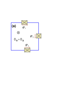
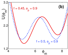
Figure 1: (Color online) (a) A three-level artificial “atom” made of a superconducting loop, with three junctions, threaded by a bias flux $\Phi_{e}$ and external field $\Phi_{a}$, consisting of the quantized and time-dependent magnetic fluxes. (b) Potential energy $U(\varphi_{p},\varphi_{m})$ versus the phase $\varphi_{m}$ for fixed $\varphi_{p}$ (e.g., $\varphi_{p}=0.9$) and reduced magnetic flux $f=\Phi_{e}/\Phi_{0}=0.5$, for the dashed blue curve, and $f=0.45$, for the continuous orange curve.

Besides the bias magnetic flux $\Phi_{e}$, we also apply another magnetic flux $\Phi_{a}$, consisting of a quantized field and two classical fields. To realize the strong coupling of the flux qubit to a quantized field, now the flux qubit is coupled to a one-dimensional transmission line resonator. This can be realized by replacing the charge-qubit in the circuit QED architecture liu-epl ; wallraff ; liu-pra ; yliu by a flux qubit. Then a single-mode quantized magnetic field can be provided by the transmission line resonator. All three fields are assumed to induce transitions among the lowest three energy levels of the artificial atom to form the $\Delta$-shaped configuration mentioned above. The frequencies of the quantized and two classical fields are assumed to be $\,\omega$, $\Omega_{e}$, and $\,\Omega_{c}$, respectively.

The Hamiltonian of the three-level artificial atom interacting with the three fields can be written as

$$H = \omega_{e}|e\rangle\langle e|+\omega_{c}|c\rangle\langle c|+\omega a^{\dagger}a$$

$$+ (g|e\rangle\langle c|a+Ge^{i\Omega_{e}t}|b\rangle\langle e|+\lambda e^{i\Omega_{c}t}|b\rangle\langle c|+{\rm H.c.}).$$

Here, we take $\hbar=1$. The quantized field is assumed to couple the transition between $|e\rangle$ and $|c\rangle$, while the two classical fields are applied between $|e\rangle$ and $|b\rangle$, as well as between $|c\rangle$ and $|b\rangle$, respectively. $\omega_{e}$ ($\omega_{c}$) are transition frequencies between $|e\rangle$ ($|c\rangle$) and $|b\rangle$ (see the Fig. 2). The detuning between the transition frequency $\omega_{e}$ (or $\omega_{c}$) and the frequency of the classical field $\Omega_{e}$ (or $\Omega_{c}$) is denoted by

$$\Delta_{e}=\omega_{e}-\Omega_{e}\,\,\,\,{\rm or}\,\,\,\,\Delta_{c}=\omega_{c}-\Omega_{c}.$$ (6)

$a$ and $a^{\dagger}$ are the annihilation and creation operators of the quantized mode, $G$ and $\lambda$ are the Rabi-frequencies of the classical fields, $g$ denotes the vacuum Rabi-frequency of the quantized mode. Without loss of generality, we assume that all Rabi frequencies are real numbers. Here, we assume that the frequencies of the three fields satisfy the condition

$$\Omega_{e}-\Omega_{c}=\omega.$$ (7)

This condition is required such that the equivalent Hamiltonian in a “rotating” reference frame (defined below) will be time-independent. In this case, the evolution of the quantum system will remain in the adiabatic subspace when the Rabi frequencies are adiabatically changed to transfer the quantum information, carried by photons, to the artificial atoms.

Figure 2 illustrates the transitions induced by the interactions of the artificial atom with the three fields. This cyclic or $\Delta$-shaped transitions define a new type of atom, different from the $\Lambda$ (or $\Xi$, or $V$)-type atoms scullybook ; jpm . In a “rotating” reference frame of a time-dependent unitary transformation

$$W(t)=\exp[-it(\Omega_{e}|e\rangle\langle e|+\Omega_{c}|c\rangle\langle c|+\omega a^{{\dagger}}a)],$$ (8)

the Hamiltonian in Eq. (II) can be rewritten as

$$H = \Delta_{c}\,|c\rangle\langle c|+\Delta_{e}\,|e\rangle\langle e|$$ (9)

$$+ (g\,|e\rangle\langle c|a+G\,|e\rangle\langle b|+\lambda\,|b\rangle\langle c|+{\rm H.c.}),$$

where the the frequencies-matching condition $\Omega_{e}-\Omega_{c}=\omega$ has been used.

The population of the three-level artificial atom can be cyclically transferred by adiabatically applying three classical fields liu . However, in the presence of a quantized field, the transitions

$$|e,n\rangle \leftrightarrow |c,n+1\rangle\leftrightarrow|b,n+1\rangle$$

$$\leftrightarrow |e,n+1\rangle\leftrightarrow|c,n+2\rangle\leftrightarrow|e,n+2\rangle\,\cdots$$

cannot form a closed cycle because each cycle produces a one photon excitation. The triangular or $\Delta$-shaped geometry of the transitions is shown in Fig. 3, where the classical fields can only induce transitions in the plane of each triangle of atom-photon joint states, while the quantized field drives the transitions from one plane to another, by increasing or decreasing one photon.

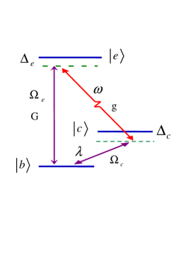
Figure 2: (Color online). Triangle- or $\Delta$-shaped transitions among three energy levels of the “artificial atom”. The classical fields with frequencies $\Omega_{e}$ and $\Omega_{c}$ induce the transitions $(G,\,\lambda)$ with Rabi frequencies $G$ and $\lambda$, while the quantized field with frequency $\omega$ induces the transition with Rabi frequency $g$.

III Mechanism to generate nonclassical photon states

In this section, we will consider the possibility to utilize the above $\Delta$-shaped three level artificial atom as a basic single photon device. It is well known that there has been considerable interest in the generation of non-classical light using solid-state devices for highly sensitive metrology and quantum information. Some solid-state lasers have been proposed to emit non-classical light with photon number squeezing, but the present proposal, based on $\Delta$-shaped artificial atoms, is essentially a macroscopic quantum device, which, in principle, could be easily controlled by only using classical parameters (e.g., the magnetic flux).

Figure 3: (Color online). Each triangle has a different number (e.g., 1, 2, 3) of photons. The classical fields can only induce in-plane transitions to form CT. The quantum field links different triangle planes to generate photons.

To intuitively describe the main mechanism of how to create the quasi-classical and non-classical photon states by using the transition configuration shown in Fig. 3, we first rewrite the sub-Hamiltonian in Eq. (9)

$$H_{s}=\Delta_{c}\,|c\rangle\langle c|+[\lambda|c\rangle\langle b|+{\rm H.c.}],$$ (10)

into

$$H_{s}=\epsilon_{+}\,|+\rangle\langle+|+\epsilon_{-}\,|-\rangle\langle-|$$ (11)

with two dressed states

$$\left|+\right\rangle = \cos\left(\frac{\theta}{2}\right)\left|c\right\rangle+\sin\left(\frac{\theta}{2}\right)\left|b\right\rangle,$$

$$\left|-\right\rangle = -\sin\left(\frac{\theta}{2}\right)\left|c\right\rangle+\cos\left(\frac{\theta}{2}\right)\left|b\right\rangle,$$

where we have defined the mixing angle

$$\theta=\arctan\left(\frac{2\lambda}{\Delta_{c}}\right).$$ (12)

It is obvious that $\theta$ can be controlled through the detuning $\Delta_{c}$ by changing the frequency of the classical field. The states $\left|\pm\right\rangle$ are the eigenstates of $H_{s}$ corresponding to the eigenvalues

$$\epsilon_{\pm}=\frac{\Delta_{c}}{2}\pm\omega^{\prime},$$ (13)

with the dressed frequency

$$\omega^{\prime}=\sqrt{\lambda^{2}+\frac{\Delta_{c}^{2}}{4}}.$$ (14)

Then, in this dressed basis, the total Hamiltonian in Eq. (9)

$$H=H_{0}+H_{1}$$ (15a)

can be rewritten as

$$H_{0}=\Delta_{e}\,|e\rangle\langle e|+\epsilon_{+}\,|+\rangle\langle+|+\epsilon_{-}\,|-\rangle\langle-|\,$$ (15b)

and

$$H_{1}=g(\theta)A\,|e\rangle\langle+|-G(\theta)B\,|e\rangle\langle-|+{\rm H.c.}$$ (15c)

with the displaced boson operators $$A=a+\xi B=A-\zeta$$ and , and the controllable parameters

$$g(\theta)=g\cos\left(\frac{\theta}{2}\right), G(\theta)=g\sin\left(\frac{\theta}{2}\right),$$

$$\xi(\theta)=\frac{G}{g}\tan\left(\frac{\theta}{2}\right), \zeta(\theta)=\frac{G}{g}\tan^{-1}\left(\frac{\theta}{2}\right).$$

The Hamiltonian (15a) describes the $\Lambda$-like transition atom shown in Fig. 4(a). Instead of the usual $\Lambda$-type atom, the transitions between states $|e\rangle$ and $|-\rangle$ are induced by two fields, one is a quantized light field with coupling strength $g\sin(\theta/2)$, described by a displaced annihilation operator $a$, another is a classical field with the Rabi frequency $G\cos(\theta/2)$.

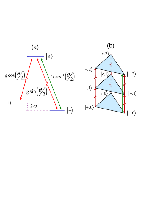
Figure 4: (Color online) Three-level artificial atom in the classical-field dressed picture. (a) A $\Lambda$-like atom equivalent to the $\Delta$-atom in Fig. 2 with the $|+\rangle\leftrightarrow|e\rangle$ transition coupled, via the left zig-zag-line, to a displaced quantized field, denoted by the operator $A$ in Eq. (15c). The $|-\rangle\leftrightarrow|e\rangle$ transition couples both an equivalent classical field, denoted by $\eta$, and a displaced quantized field $A$ in Eq. (15c). (b) After doing adiabatic elimination for large detuning, there are no transitions among the three energy levels in the same equal-number-of-photons triangle-plane. The vertical arrowed lines linking the vertices of the triangles represent the transitions that accompany the creation of photons.

Figure 4(a) schematically describes the creation of quasi-classical and non-classical photon states based on the CT process. Due to the coherent $|c\rangle$-$|b\rangle$ interaction with the coupling strength $\lambda$, as in Eq. (10), the system can be described by the driven JC model shown in Eq. (15a). However, for large detunings, in Eqs. (15a-15c), i.e., $\Delta_{e}-\epsilon_{\pm}\gg g(\theta),\,G(\theta)$, we can adiabatically separate the excited state $|e\rangle$ and then a coherent transition between states $|c\rangle$ and $|b\rangle$ is induced by the quantized field originally applied between $|e\rangle$ and $|c\rangle$. This is very similar to the usual Jaynes-Cummings (JC) model, obtained by adiabatically eliminating the highest third energy level in the stimulated Raman scattering of intense laser light. In the dressed states $|\pm\rangle$ basis, and for the above large detuning condition, there exist three types of subspaces, related to states $|+\rangle$, $|-\rangle$, and $|e\rangle$, respectively. These subspaces are depicted in Fig. 4(b) by vertical lines linking the vertices of the triangles. Corresponding to each state, e.g., $|+\rangle$, the photon mode is driven by an effective external force depending on the coherent $|c\rangle$-$|b\rangle$ interaction, and thus the single mode photon states can be produced from the vacuum state.

IV Adiabatic generation of Schrödinger cat states

In order to better understand the above-mentioned mechanism to generate non-classical photon states from these controllable artificial atoms, we demonstrate the adiabatic generation of Schrödinger cat states. In the large detuning limit, we can adiabatically eliminate the terms causing transitions from $|e\rangle$ to $|+\rangle$ and $|-\rangle$.

The adiabatic elimination can be done by using the Fröhlich-Nakajima transformation (FNT) fro ; nakajima , which is applied to achieve the effective electron-electron interaction Hamiltonian in the BCS theory. To consider the validity of this method, we will show that it is equivalent to a result of the second order perturbation in the Appendix A. In the FNT method, we define a transformation by the operator $V=$ $\exp(S)$, with an anti-Hermitian operator $S$ to be determined. Then we apply this transformation $V$ to the original Hamiltonian (15a) to given an equivalent Hamiltonian $H_{V}=V^{\dagger}HV.$

We assume that the operator $S$ to be the perturbation term with the same order as $H_{I}$, and then we can expand $H_{V}$ in the series of $S$. In general, we can consider the Hamiltonian of an interacting system, described by a sum of free Hamiltonian $H_{0}$ and the interaction Hamiltonian $H_{1}$ as $H=H_{0}+H_{1}$, shown in Eq. (15a). By comparing with the free part $H_{0}$, the interaction part $H_{1}$ can be regard as a perturbation term. Let us perform the transformation $V=$ $\exp(S)$ on the Hamiltonian $H=H_{0}+H_{1}$. Then, we can derive an approximately equivalent Hamiltonian $H_{V}$ as

$$H_{V}\cong H_{0}+\frac{1}{2}\left[H_{1},\,S\right],$$ (16)

where the operator $S$ can be determined by

$$H_{1}+[H_{\mathrm{0}},S]=0.$$ (17)

The transformation, by which one can obtain the effective Hamiltonian in Eq. (16) from the Hamiltonian in Eq. (15a), is the so-called generalized Fröhlich transformation (for details, see Appendix A).

If we replace $H_{0}$ and $H_{1}$ in Eq. (17) by the explicit expressions in Eqs. (15b) and (15c), and assume

$$S = \Gamma_{1}\,A\,|e\rangle\langle+|+\Gamma_{2}\,B\,|e\rangle\langle-|$$ (18)

$$+ \Gamma_{3}\,A^{\dagger}\,|+\rangle\langle e|+\Gamma_{4}\,B^{\dagger}\,|-\rangle\langle e|,$$

for parameters $\Gamma_{i}\,(i=1,\,2,\,3,\,4)$ to be determined, then the parameters $\Gamma_{i}\,(i=1,\,2,\,3,\,4)$ can be obtained as

$$\Gamma_{1} = -\Gamma_{3}\,=\,-\frac{g(\theta)}{\epsilon+\Delta},$$ (19a)

$$\Gamma_{2} = -\Gamma_{4}\,=\,-\frac{G(\theta)}{\epsilon-\Delta},$$ (19b)

with

$$\Delta=\frac{1}{2}\sqrt{(\Delta_{c}-\Delta_{e})^{2}+4\lambda^{2}},\,\,\,\epsilon=\frac{1}{2}(\Delta_{c}+\Delta_{e}).$$ (20)

Then, using the expressions of $S$, $H_{0}$, and $H_{1}$ in Eqs. (18), (15b), and (15c), we can obtain an effective Hamiltonian from Eq. (16) as

$$H_{V}\approx H_{e}|e\rangle\langle e|+H_{bc}.$$ (21a)

Here, the Hamiltonians $$H_{e} H_{bc}$$ and can be expressed as

$$H_{e}=\Delta_{e}+\Omega_{A}\,A\,A^{+}+\Omega_{B}\,B\,B^{+}$$ (21b)

and

$$H_{bc} = (\epsilon_{+}-\Omega_{A}A^{+}A)|+\rangle\langle+|$$ (21c)

$$+(\epsilon_{-}-\Omega_{B}B^{+}B)|-\rangle\langle-|$$

$$+\Gamma[AB^{+}|+\rangle\langle-|+A^{+}B|-\rangle\langle+|],$$

with

$$\Gamma=\frac{G(\theta)g(\theta)}{2\Delta_{-}\Delta_{+}}(2\Delta_{e}-\Delta_{c}).$$ (22)

The effective frequencies

$$\Omega_{A}=\frac{g^{2}(\theta)}{\Delta_{+}},\,\,\,\,\Omega_{B}=\frac{G^{2}(\theta)}{\Delta_{-}}$$ (23)

represent the Stark shifts with $\Delta_{\pm}=\Delta_{e}-\epsilon_{\pm}$.

According to former definitions of the operators $A$ and $B$ in Eq. (15c), the Hamiltonian $H_{e}$ can be rewritten as

$$H_{e} = (\Omega_{A}+\Omega_{B})\,a\,a^{\dagger}$$

$$+[(\xi\,\Omega_{A}-\eta\,\Omega_{B})\,a^{\dagger}+{\rm H.c.}]$$

after neglecting the constant terms $\Delta_{e}+|\xi|^{2}+|\eta|^{2}$. It is clear that the Hamiltonian $H_{e}$ describes a driven harmonic oscillator. Then, when the total system can be adiabatically kept in the excited state $|e\rangle$, $H_{e}$ describes the creation of a coherent photon state from the vacuum scullybook . However, due to the spontaneous emission of excited states, it is difficult to keep the artificial atom in its excited state $|e\rangle$. Thus, let us now consider how to generate non-classical photon states by only using the more robust lower states $|\pm\rangle$.

The last term in $H_{bc}$ oscillates in a larger frequency range: $|\epsilon_{+}-\epsilon_{-}|\simeq 2\omega^{\prime}$. Thus, in the rotating wave approximation, we have

$$H_{bc} = (\epsilon_{+}-\Omega_{A}A^{+}A)|+\rangle\langle+|$$ (25)

$$+ (\epsilon_{-}-\Omega_{B}B^{+}B)|-\rangle\langle-|.$$

This is the standard Hamiltonian to describe the dynamical generation of Schrödinger cat states (e.g., Ref. cqed ). Since the bare ground state $|b\rangle$ is easy to be initialized, we can assume that the artificial atom is initially in the bare ground state $|b\rangle=\sin(\theta/2)|+\rangle+\cos(\theta/2)|-\rangle$, while the cavity field is initially in the vacuum state $|0\rangle$. Then at time $\tau$, the whole system can evolve into

$$|\psi(\tau)\rangle\,\, = \exp(iH_{bc}t)[\sin(\theta/2)|+\rangle+\cos(\theta/2)|-\rangle]|0\rangle$$ (26)

$$= \sin\frac{\theta}{2}\exp[i\xi^{2}\exp(-i\Omega_{A}t)]|\alpha(-\xi,t)\rangle|+\rangle$$

$$+ \cos\frac{\theta}{2}\exp[i\zeta^{2}\exp(-i\Omega_{B}t)]|\alpha(\zeta,t)\rangle|-\rangle.$$

where $|\alpha(x,t)\rangle=$ $|\alpha=\alpha(x,t)\rangle$ (and $x=\xi,\zeta$) denotes coherent states with

$$\alpha(x,t)=x[1-\exp(i\Omega_{x}t)]$$ (27)

and $\Omega_{\xi}=\Omega_{A,}$ $\Omega_{\zeta}=\Omega_{B}$. By adjusting the coupling constant $\lambda$ between $|c\rangle$ and $|b\rangle$, in this “cyclic atom”, one can control dynamical processes to obtain the cat states of the qubit subsystem consisting of the two dressed states $|\pm\rangle$ entangled with the quantized field.

To show the existence of the “cat”, we need to calculate the overlap

$$F(\lambda,t)=|\langle\alpha(\zeta,t)|\alpha(-\xi,t)\rangle|=\exp[-y(\lambda,t)]$$ (28)

for two coherent states $|\alpha(-\xi,t)\rangle$ and $|\alpha(\zeta,t)\rangle$, where

$$y(\lambda,t) = 2(\zeta+\xi)^{2}-4\zeta\xi\sin^{2}\left[\frac{t}{2}(\Omega_{B}-\Omega_{A})\right]$$

$$-2\zeta(\zeta+\xi)\cos(\Omega_{B}t)-2\xi(\zeta+\xi)\cos(\Omega_{A}t).$$

In Fig. 5, the time evolution of $y(t)$ is plotted for given parameters, e.g., $\Delta_{e}=3\lambda$, $G=0.9\lambda$, $g=0.8\lambda$ for different values of $\theta=\arctan(2\lambda/\Delta_{c})=\pi/2,\,\,\pi/4,\,\,\pi/6$. It shows that $y(t)$ can periodically reach its maximum value, which means that $|\langle\alpha(\zeta,t)|\alpha(-\xi,t)\rangle|$ becomes minimum at these times, with period $2\pi$. The period of the function $y(t)$ is determined by three frequencies $\Omega_{A}$, $\Omega_{B}$, and $\Omega_{B}-\Omega_{A}$, so Fig. 5 shows the small modulation overimposed on the larger modulation. We find that a larger detuning $\Delta_{c}$ corresponds to a larger maximum value when other parameters are fixed. However, $y(t)$ needs a longer period to reach these maximum points. The above result demonstrates that macroscopic Schrödinger cat states, an entanglement between a macroscopic quantum two-level system (macroscopic qubit) and the non-classical photon states, can be generated by superconducting quantum devices. These cat states are different from the usual Schrödinger cat states, an entanglement between a microscopic two level atom and the quasi-classical photon states, which are created by using the atomic cavity QED cqed .

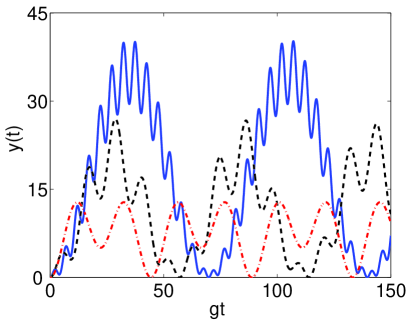
Figure 5: (Color online). The exponent $y(t)$, see Eqs. (28) and  (IV), of the overlap of two coherent states is plotted as a function of $gt$, see Eqs. (23),  (28) and  (IV) for given parameters $\Delta_{e}=3\lambda$, $G=0.9\lambda$, $g=0.8\lambda$, $\theta=\pi/2$ (dash-dotted red curve), $\theta=\pi/3$ (dotted black curve), and $\theta=\pi/4$ (solid blue curve).

The above setup can also be used to create a coherent state if the cyclic artificial atom is initially prepared in the state $|-\rangle$. In this case, the total system should be adiabatically kept in the ground state $|-\rangle$. The effective Hamiltonian becomes $H_{-}\simeq-\Omega_{B}B^{+}B$, by dropping the constant term. More explicitly,

$$H_{-}\simeq-\Omega_{B}a^{+}a+f(\theta)(a+a^{+})$$ (30)

realizes a driven harmonic oscillator. The driving force $f(\theta)$ can be expressed as $f(\theta)=G(\theta)g(\theta)/\Delta_{-}$, and it depends on the coupling constant $\lambda$. Starting from the vacuum $|0\rangle$, with a duration $t$, the single-mode quantized field will evolve into a coherent state $|\varphi(t)\rangle=|\alpha\rangle$ with $\alpha=\zeta[1-\exp(i\Omega_{B}t]$, where a time-dependent global phase $\exp[i\zeta^{2}(\sin(\Omega_{B}t)-\Omega_{B}t)]$ has been neglected. From the expression of the photon number

$$N(t)\,=\,\langle\alpha|a^{+}a|\alpha\rangle\,=\,\zeta^{2}|1-\exp(i\Omega_{B}t))|^{2},$$ (31)

we can calculate the generation rate of the photons in the quantized mode:

$$r(t)\,=\,\left|\frac{\mathrm{d}N(t)}{\mathrm{d}t}\right|=\frac{2g^{2}(\theta)}{\Delta_{-}}\sin(\Omega_{b}t).$$ (32)

This result shows that, the coupling strength $\lambda$ of the interaction between $\left|c\right\rangle$ and $\left|b\right\rangle$, caused by the symmetry-breaking, can be used to enhance the probability of creating single-mode photons. If there is no interaction between $|c\rangle$ and $|b\rangle$, the external force $f(\theta)$ would vanish accordingly and then the dynamic evolution cannot automatically produce coherent photon states.

V Conclusions

In an artificial atom represented by a superconducting quantum circuit, we briefly review optical transitions and their selection rules. It is shown that all transitions are possible in such artificial atom when the applied bias magnetic flux is not at the optimal point liu . Then cyclic or $\Delta$-shaped transitions can be realized for the lowest three energy levels in this artificial atom. Using this cyclic population transfer mechanisms, we have studied how to create nonclassical single-mode photon states and a macroscopic Schrödinger cat states. We show that this approach is controllable, because either the ground state or the two lowest-energy levels are utilized through their coherent coupling to external fields, which can be used to control the parameters of the system. For example, if the Rabi frequency $\lambda=0$, then the classical field, which induces transitions between states $|c\rangle$ and $|b\rangle$, is set to zero. Thus, our model can be referred to $\Lambda-$type atom driven by a quantized and a classical fields parkins . In this case parkins , neither the cat state nor the coherent state can be generated from the initial state of the whole system with the bare ground state of atom and the vacuum of the quantized field. Starting from either the vacuum or a coherent state, it is a deterministic scheme to generate nonclassical photon states via CT manipulations.

The large detuning limit implies a relatively weak coupling constants $g(\theta)$ and $G(\theta)$, as well as relatively large detuning $\Delta_{e}-\epsilon_{\pm}$, shown in Eqs. (15b-15c). Thus it limits the efficient adjustment of the dynamic processes. Therefore, a generic version of our proposal might not be very efficient. Fortunately, in our proposal, the strength $\lambda$ of the controlling-field coupling between $|c\rangle$ and $|b\rangle$ is adjustable. Thus, one can feasibly manipulate this parameter for our goal without violating the requirement of large detuning.

Another question is the problem of decoherence. An efficient scheme requires the decoherence time comparable with the characteristic time of the effective frequencies $\Omega_{B}$ and $\Omega_{A}$. It is known that the interaction strength $g$ between the qubit and quantized field can reach about $100$ MHz if we use the transmission line resonator in the circuit QED gir ; wallraff . According to the definitions of $\Omega_{B}$ and $\Omega_{A}$ in Eq. (23), they can be of the order of $10-100$ MHz, if we choose appropriate detunings $\Delta_{e}$ and $\Delta_{c}$. Then, it is possible to realize our proposal within the experimental values gir1 for $T_{1}\sim 7\,\mu$s and  $T_{2}\sim 800$ ns.

Finally, we should point out the relation between our present work and the quantum Carnot engine (QCE) in Ref. scully ; quan . In the QCE proposal, the $\Lambda$-type atoms are prepared as a superposition of two lower states. In the $\Delta$-type transition configuration, the superposition of the two lowest states can be naturally produced by the interaction between the field and the artificial atom, and hence the cyclic three-level atom is a good candidate to demonstrate the QCE.

VI Acknowledgments

We acknowledge the partial support of the US NSA and ARDA under AFOSR contract No. F49620-02-1-0334, and the NSF grant No. EIA-0130383. The work of CPS is also partially supported by the NSFC and Fundamental Research Program of China with No. 2001CB309310.

Appendix A Generalized Fröhlich-Nakajima transformation and its equivalence to perturbation theory

Let us consider a Hamiltonian $H$ of a given system with its free part $H_{0}$ and a perturbation term $H_{I}$

$$H=H_{0}+\lambda H_{I}.$$ (33)

Here, $\lambda$ is the so-called perturbation parameter introduced to characterize the order of the perturbation. At the end of calculation, $\lambda$ is taken as unity.

The crucial point of the generalized Fröhlich-Nakajima transformation is to choose a proper unitary transformation $V(\lambda)=\exp(\lambda S)$, where $S$ is an anti-Hermitian operator, to be determined. The inverse transformation of $V(\lambda)$ makes the states $|\Psi\rangle$, governed by the Hamiltonian in Eq. (33), change to a new state

$$|\Phi\rangle=V(-\lambda)|\Psi\rangle=\exp(-\lambda S)|\Psi\rangle.$$ (34)

And the evolution of the state $|\Phi\rangle$ is governed by the transferred Hamiltonian

$$H_{\lambda}=e^{-\lambda S}He^{\lambda S}.$$ (35)

It is well known that the unitary transformation does not change the dynamics of the system, and then the Hamiltonians $H_{\lambda}$ and $H$ describe the same physical process. Here the operator $S$ should be appropriately chosen such that it has the same order as the perturbation term $H_{I}$. Physically, the effect of the Hamiltonian $H_{I}$ on the final result is so small that it can be neglected.

Using the Baker-Campbell-Hausdorff formula, the Hamiltonian $H_{\lambda}$ can be expressed in a series of the parameter $\lambda$ as

$$H_{\lambda}=H_{0}+\sum_{n=1}\frac{\lambda^{n}(-1)^{n-1}}{(n-1)!}{\underset{n-1}{\underbrace{[S,\,[S,\,\cdots[S}},\,\,H_{I}]]]}.$$ (36)

Second order perturbation theory can be realized by imposing the condition

$$H_{I}+\left[H_{0},S\right]=0$$ (37)

on Eq. (36). Eq. (37) can be used to determine the operator $S$. For the sake of simplicity, the eigenstates of $H_{0}$ are assumed to be non-degenerate. Let $|n\rangle$ be the eigenstate of the Hamiltonian $H_{0}$ with the eigenvalue $E_{n}$. Taking the matrix elements of Eq. (37 ) with respect to the basis $\{|n\rangle\}$ as

$$\langle m|H_{I}|n\rangle+\left(E_{m}-E_{n}\right)\langle m|S|n\rangle=0,$$ (38)

we can find the explicit expression of matrix elements for the operator $S$

$$S_{mn}=\langle m|S|n\rangle=\frac{\langle m|H_{I}|n\rangle}{E_{n}-E_{m}}.$$ (39)

Thus, the representation of the operator $S$ in the $\{|n\rangle\}$ basis can be

$$S=\sum_{m\neq n}\frac{\langle m|H_{I}|n\rangle}{E_{n}-E_{m}}\,|m\rangle\langle n|.$$ (40)

From Eqs. (36) and (37), we obtain the effective Hamiltonian

$$H_{\lambda}\cong H_{0}+\frac{1}{2}\left[H_{I},\,S\right]$$ (41)

up to second order in $H_{I}$. Using a matrix representation, $H_{\lambda}$ can be expressed as

$$H_{\lambda} = \sum_{n}E_{n}|n\rangle\langle n|$$ (42)

$$+ \sum_{l\,(l\neq n),\,m}\frac{\langle m|H_{I}|l\rangle\,\langle l|H_{I}|n\rangle}{2(E_{n}-E_{l})}\,|m\rangle\langle n|$$

in the $\{|n\rangle\}$ basis. We can see that the Fröhlich-Nakajima transformation is only applicable to a systems with $\langle m|H_{I}|m\rangle=0$. Actually we can decompose the total Hamiltonian $H$ such that $H_{0}$ only includes all diagonal elements in the $\{|n\rangle\}$ basis of eigenstates for the Hamiltonian $H_{0}$ while the off-diagonal ones are included in $H_{I}$.

It is easy to obtain the eigenvalues of the transferred Hamiltonian in Eq. (41) or (42), up to second order in $H_{I}$, as

$$E_{n}^{(0)} = \langle n|H_{0}|n\rangle+\frac{1}{2}\langle n|\left[H_{I},\,\,S\right]|n\rangle$$ (43)

$$= E_{n}+\sum_{l\neq n}\frac{|\langle l|H_{I}|n\rangle|^{2}}{E_{n}-E_{l}},$$

which correspond to the zero-order eigenstates of the Hamiltonian $H_{\lambda}$. The second term in the right side of Eq. (43) is the so-called self-energy term.

In fact, from Eq. (42), it can be found that zero-order eigenstates $|\Psi_{n}^{(0)}\rangle$ of the Hamiltonian $H_{\lambda}$ are just the eigenstates $|n\rangle$ of the Hamiltonian $H_{0}$, i.e., $|\Psi_{n}^{(0)}\rangle=|n\rangle$. The eigenvalues in Eq. (43) provide energy corrections using the time-independent perturbation theory.

To consider the relation between the Fröhlich-Nakajima transformation and the time-independent perturbation theory, we can transfer eigenstates $|\Psi_{n}^{(0)}\rangle$ back to the original picture. In this case, the first order eigenstates $|\Psi_{n}^{(1)}\rangle$ of the Hamiltonian $H$ can be obtained by

$$|\Psi_{n}^{(1)}\rangle = V\left(\lambda\right)|\Psi_{n}^{(0)}\rangle=\left(1+S\right)|n\rangle$$

$$= |n\rangle+\sum_{m\neq n}\frac{\langle m|H_{I}|n\rangle}{E_{n}-E_{m}}|m\rangle,$$

where the expansion $V\left(\lambda\right)$ is kept up to first order in $\lambda$.

It is easy to prove that $|\Psi_{n}^{(1)}\rangle$ are just the first-order eigenstates of the original Hamiltonian $H$, with respect to the perturbation decomposition of $H_{0}$ and $H_{I}$. Since we have chosen that $H_{I}$ does not have diagonal terms, the first correction to the energy is zero, and then $E_{n}$ is also the result of the first correction of the energy for the Hamiltonian $H$.

The eigenvalues in Eq. (43) are up to the second order corrections. Correspondingly, the eigenstates $|\Psi_{n}^{(2)}\rangle$ of $H$ corresponding to the second-order energy corrections can be given by acting $V(\lambda)$ on the first order eigenstates $|\Psi_{n}^{(1)}\rangle$ of the Hamiltonian $H_{\lambda}$. That is

$$|\Psi_{n}^{(2)}\rangle = V(\lambda)\,|\Phi_{n}^{(1)}\rangle=V^{-1}(\lambda)\,|\Psi_{n}^{(1)}\rangle$$

$$= \left(1+S+\frac{S^{2}}{2}\right)|\Psi_{n}^{(1)}\rangle$$

$$= |n\rangle+\sum_{m\neq n}\frac{\langle m|H_{I}|n\rangle}{E_{n}-E_{m}}|m\rangle$$

$$+ \sum_{l,\,m,\,l\neq n}\frac{\langle m|H_{I}|l\rangle\langle l|H_{I}|n\rangle}{2\left(E_{l}-E_{m}\right)\left(E_{n}-E_{l}\right)}|m\rangle.$$

References

- (1) M. O. Scully and M. S. Zubairy, Quantum Optics (Cambridge University Press, Cambridge, 1997).
- (2) J. P. Marangos, J. Mod. Optics 45, 471 (1997); K. Bergmann, H. Theuer, and B. W. Shore, Rev. Mod. Phys. 70, 1003 (1998).
- (3) P. Král and M. Shapiro, Phys. Rev. Lett. 87, 183002 (2001); P. Král, I. Thanopulos, M. Shapiro, and D. Cohen, ibid. 90, 033001 (2003); I. Thanopulos, P. Král, and M. Shapiro, ibid. 92, 113003 (2004).
- (4) M. Fleischhauer, R. Unanyan, B. W. Shore, and K. Bergmann, Phys. Rev. A 59, 3751 (1999); R. Unanyan, L. P. Yatsenko, K. Bergmann, and B. W. Shore, Opt. Comm. 139, 49 (1997).
- (5) Yu-xi Liu, J. Q. You, L. F. Wei, C. P. Sun, and F. Nori, Phys. Rev. Lett. 95, 087001 (2005).
- (6) Z. Zhou, S. I. Chu, and S. Han, Phys. Rev. B 66, 054527 (2002); ibid. 70, 094513 (2004); C. P. Yang and S. Han, Phys. Rev. A 70, 062323 (2004).
- (7) N. Aravantinos-Zafiris and E. Paspalakis, Phys. Rev. A 72, 014303 (2005).
- (8) R. Migliore and A. Messina, Phys. Rev. B 67, 134505 (2003).
- (9) K. V. R. M. Murali, Z. Dutton, W. D. Oliver, D. S. Crankshaw, and T. P. Orlando, Phys. Rev. Lett. 93, 087003 (2004).
- (10) J. Q. You and F. Nori, Phys. Today 58, Vol. 11, 42 (2005).
- (11) T.P. Orlando, J. E. Mooij, L. Tian, C. H. van der Wal, L. S. Levitov, S. Lloyd, and J. J. Mazo, Phys. Rev. B 60, 15398 (1999); J. E. Mooij, T. P. Orlando, L. Levitov, L. Tian, C. H. van der Wal, and S. Lloyd, Science 285, 1036 (1999); C. H. van der Wal, A. C. J. ter Haar, F. K. Wilhelm, R. N. Schouten, C. J. P. M. Harmans, T. P. Orlando, S. Lloyd, and J. E. Mooij, Science 290, 773 (2000); I. Chiorescu, Y. Nakamura, C. J. P. M. Harmans, and J. E. Mooij, ibid. 299, 1869 (2003).
- (12) Y. Yu, D. Nakada, J. C. Lee, B. Singh, D. S. Crankshaw, T. P. Orlando, K. K. Berggren, and W. D. Oliver, Phys. Rev. Lett. 92, 117904 (2004).
- (13) S. Saito, M. Thorwart, H. Tanaka, M. Ueda, H. Nakano, K. Semba, and H. Takayanagi, Phys. Rev. Lett. 93, 037001 (2004).
- (14) J. Q. You and F. Nori, Phys. Rev. B 68, 064509 (2003).
- (15) A. Wallraff, D. I. Schuster, A. Blais, L. Frunzio, R. S. Huang, J. Majer, S. Kumar, S. M. Girvin, and R. J. Schoelkopf, Nature 431, 162 (2004); A. Blais, R. S. Huang, A. Wallraff, S. M. Girvin, and R. J. Schoelkopf, Phys. Rev A 69, 062320 (2004).
- (16) Yu-xi Liu, L. F. Wei, and F. Nori, Phys. Rev. A 71, 063820 (2005); ibid. 72, 033818 (2005).
- (17) Yu-xi Liu, L. F. Wei, and F. Nori, Europhys. Lett. 67, 941 (2004).
- (18) H. Fröhlich, Phys. Rev. 79, 845 (1950).
- (19) S. Nakajima, Adv. Phys. 4, 463 (1953).
- (20) M. Brune, E. Hagley, J. Dreyer, X. Maitre, A. Maali, C. Wunderlich, J. M. Raimond, and S. Haroche, Phys. Rev. Lett. 77, 4887 (1996).
- (21) A. S. Parkins, P. Marte, and P. Zoller, and H. J. Kimble, Phys. Rev. Lett. 71, 3095 (1993); A. S. Parkins, P. Marte, P. Zoller, O. Carnal and H. J. Kimble, Phys. Rev. A 51, 1578 (1995). B. W. Shore, J. Martin, M. P. Fewell, and K. Bergmann, Phys. Rev. A 52, 566 (1995); J. Martin, B. W. Shore, and K. Bergmann, Phys. Rev. A 54, 1556 (1996).
- (22) J. Q. You, J. S. Tsai, and F. Nori, Phys. Rev. B 68, 024510 (2003).
- (23) A. Wallraff, D. I. Schuster, A. Blais, L. Frunzio, J. Majer, M. H. Devoret, S. M. Girvin, and R. J. Schoelkopf, Phys. Rev. Lett. 95, 060501 (2005).
- (24) M. O. Scully, M. S. Zubairy, G. S. Agarwal, and H. Walther, Science 299, 862 (2003); H. Linke, ibid. 299, 841 (2003).
- (25) H. T. Quan, P. Zhang, C. P. Sun, Phys. Rev. E, in press (2005).