Coherent backscattering in nonlinear atomic media: quantum Langevin approach

Abstract

In this theoretical paper, we investigate coherence properties of the near-resonant light scattered by two atoms exposed to a strong monochromatic field. To properly incorporate saturation effects, we use a quantum Langevin approach. In contrast to the standard optical Bloch equations, this method naturally provides the inelastic spectrum of the radiated light induced by the quantum electromagnetic vacuum fluctuations. However, to get the right spectral properties of the scattered light, it is essential to correctly describe the statistical properties of these vacuum fluctuations. Because of the presence of the two atoms, these statistical properties are not Gaussian : (i) the spatial two-points correlation function displays a speckle-like behavior and (ii) the three-points correlation function does not vanish. We also explain how to incorporate in a simple way propagation with a frequency-dependent scattering mean-free path, meaning that the two atoms are embedded in an average scattering dispersive medium. Finally we show that saturation-induced nonlinearities strongly modify the atomic scattering properties and, as a consequence, provide a source of decoherence in multiple scattering. This is exemplified by considering the coherent backscattering configuration where interference effects are blurred by this decoherence mechanism. This leads to a decrease of the so-called coherent backscattering enhancement factor.

I Introduction

Over the past ten years, cold atomic gases have gradually become a widely employed and highly tunable tool for testing new ideas in many areas of quantum physics: quantum phase transitions (Bose-Einstein condensation, Fermi degenerate gases, Mott-Hubbard transition) bec ; fermi ; mott-hubbard , quantum chaos chaos , applications in metrology hsurm , disordered systems cbsat ; thierry to cite a few. In the latter case, cold atomic vapors act as dilute gases of randomly distributed atoms multiply scattering an incident monochromatic laser light. In this case, the scattered light field exhibit a speckle-like structure due to (multiple) interference between all possible scattering paths. The key point is that the disorder average is insufficient to erase all interference effects. This gives rise to weak or strong localization effects in light transport depending on the strength of disorder Houches ; AkkerMon . A hallmark of this coherent transport regime is the coherent backscattering (CBS) phenomenon: the average intensity multiply scattered off an optically thick sample is up to twice larger than the average background in a small angular range around the direction of backscattering, opposite to the incoming light cbs . This interference enhancement of the diffuse reflection off the sample is a manifestation of a two-wave interference. As such, it probes the coherence properties of the outgoing light photon . The CBS effect in cold atomic gases has been the subject of extensive studies in the weak localization regime, both from theoretical and experimental points of view cbsatoms . In particular, modifications brought by atoms, as compared to classical scatterers, for light transport properties (mean-free path, coherence length, CBS enhancement factor) have been highlighted. They are essentially due to the quantum internal atomic structure internal ; cbsB .

Another interesting feature of atoms is their ability to display a nonlinear behavior: the scattered light is no more proportional to the incident one. This leads to a wide variety of phenomena, like pattern formation, four-wave mixing, self-focusing effects, dynamical instabilities, etc boyd ; prl72GMP ; praDHGC ; prl85SM . For a weak nonlinearity, introducing an intensity-dependent susceptibility is enough to properly describe these effects, including quantum properties boyd ; pra70WGDM ; facteur3 , e.g. the Kerr effect (intensity dependence of the refractive index) can be obtained with a $\chi^{(3)}$ nonlinearity. However, when the incident intensity is large enough, and this is easily achieved with atoms, perturbation theories eventually fail and a full nonlinear treatment is required. For a single two-level atom, the solution is usually given by the so-called optical Bloch (OB) equations. Together with the quantum regression theorem, they allow for a complete description of the spectral properties of the fluorescence light Cohenrouge . In particular, these equations show that the atomic nonlinear behavior is intrinsically linked to the quantum nature of the electromagnetic field. More specifically, as opposed to classical nonlinear scatterers, the radiated light exhibits quantum fluctuations characterized by peculiar time correlation properties. They define a power spectrum, known as the Mollow triplet, emphasizing inelastic scattering processes at work in the emission process pr188M ; Cohenrouge ; ZG .

However, even if all these aspects are well understood in the case of a single atom exposed to a strong monochromatic field Cohenrouge , the situation changes dramatically in the case of a large number of atoms where a detailed analysis including both quantum nonlinear properties and coherence effects is still lacking. Until now, the nonlinear coupling between the atoms and the quantum vacuum fluctuations is either included in a perturbative scheme facteur3 ; Wellens_long or simply described by a classical noise pra46YMC ; pra46YMC2 ; pra51YC ; pra52DPGC ; pra56B . In the dilute regime $\lambda\ll R$ where the light wavelength $\lambda$ is much less than the average particle separation $R$, one expects the quantum fluctuations to reduce the degree of coherence of the scattered light. This will alter not only propagation parameters (mean-free path, refraction index), but also weak localization corrections to transport, and the CBS enhancement factor, which is related to the coherence properties of the scattered light field thierry ; photon . We want here to stress that, even beyond interference and weak localization phenomena, any transport property which may be influenced by saturating the atomic transition deserves a special and necessary study on its own. The most striking systems falling in this category where both nonlinear and disordered descriptions are intimately interwoven are coherent random lasers cao where interference effects lead to localized light modes inside the disordered medium, comparable to resonator eigenmodes in standard lasers. Even if, in this case, one would require an active (i.e. amplifying) medium, a key point is the understanding of the mutual effects between multiple interferences and nonlinear scattering.

In the present paper, we will focus on the rather simple case of two atoms in vacuum. Our aim is threefold: (i) firstly to properly calculate quantum correlations between pairs of atoms as a crucial step towards a better understanding of the physical mechanisms at work; (ii) secondly to implement a method allowing for a simple incorporation of frequency-dependent propagation effects; (iii) finally to understand, in the CBS situation, the modifications brought by the (quantum) nonlinearity to the interference properties. We hope that these points, once mastered, can provide an efficient way to produce realistic computer models to simulate real experiments. Point (i) alone could easily be solved using the standard OB method pra45VA ; prl94SMB . But the latter almost becomes useless regarding point (ii), since frequency-dependent propagation leads to complicated time-correlation functions. From a numerical point of view, it also leads to such large linear systems of coupled equations that its practical use is limited up to only a few atoms, very far from a real experimental situation. For these reasons, we will rather use the quantum Langevin method for our purposes. This method not only solves points (i) and (ii), but also leads to a simple explanation of point (iii), through a direct evaluation of the quantum noise spectrum. Note however that, in the absence of any effective medium surrounding the two atoms, and as long as only the numerical results are concerned (but not the physical interpretation), the quantum Langevin approach is completely equivalent to solving the multi-atoms optical Bloch equations like in pra45VA ; prl94SMB .

This paper divides as follows: in section II, the notations are defined and the quantum Langevin approach is explained for the single atom case. In section III, the method is adapted to the case where two atoms are weakly coupled by the dipole interaction. The validity and relevance of the method is controlled by a comparison with a direct calculation using OB equations. Then, in the CBS configuration, numerical results for different values of the laser intensity and detuning are presented and discussed. In particular, possible reasons for the reduction of the enhancement factor are put forward.

II Single two-level atom case

II.1 Time-domain approach

We consider an atom with a zero angular momentum electronic ground state ($J_{g}=0$) exposed to a monochromatic light field. The light field frequency $\omega_{L}$ is near-resonant with an optical dipole transition connecting this ground state to an excited state with angular momentum $J_{e}=1$. The angular frequency separation between these two states is $\omega_{0}$ and the natural linewidth of the excited state is $\Gamma$. We will denote hereafter by $\delta=\omega_{L}-\omega_{0}$ the laser detuning. The ground state is denoted by $|0\,0\rangle$ while the excited states are denoted by $|1\,m_{e}\rangle$, with $m_{e}=-1,0,1$ the Zeeman magnetic quantum number. As we assume no magnetic field to be present throughout this paper, the excited state is triply degenerate.

In the Heisenberg picture, this two-level atom is entirely characterized by the following set of 16 time-dependent operators:

$$\Pi^{g}=|0\,0\rangle\langle 0\,0|\quad;\quad\Pi^{e}_{m_{e}\,m^{\prime}_{e}}=|1\,m_{e}\rangle\langle 1\,m^{\prime}_{e}|\quad;\quad\mathcal{D}^{+}_{m_{e}}=|1\,m_{e}\rangle\langle 0\,0|\quad;\quad\mathcal{D}^{-}_{m_{e}}=|0\,0\rangle\langle 1\,m_{e}|$$ (1)

The atomic operators obey the completeness constraint

$$\openone=\Pi^{g}+\Pi^{e}$$ (2)

where $\Pi^{g}$ and $\Pi^{e}=\sum_{m_{e}}\Pi^{e}_{m_{e}\,m_{e}}$ are the ground and excited state atomic population operators.

The full atom-field Hamiltonian $\mathcal{H}$ is the sum of the free atom Hamiltonian $\mathcal{H}_{A}=\hbar\omega_{0}\Pi^{e}$, of the free quantized field Hamiltonian $\mathcal{H}_{F}=\sum_{\textbf{k},\boldsymbol{\epsilon}\perp\textbf{k}}\hbar\omega_{\textbf{k}}\,a^{\dagger}_{\textbf{k}\boldsymbol{\epsilon}}a_{\textbf{k}\boldsymbol{\epsilon}}$ and of the dipolar interaction $\mathcal{V}=-\mathbf{d}\cdot(\mathbf{E}_{L}+\mathbf{E}_{V})$ between the atomic dipole $\mathbf{d}$, the classical laser field $\mathbf{E}_{L}$ and the quantum electromagnetic vacuum field $\mathbf{E}_{V}$. Performing the usual approximations of quantum optics, i.e. neglecting non-resonant terms (rotating wave approximation) and assuming Markov-type correlations between the atomic operators and the vacuum field, one obtains the quantum Langevin equations controlling the time evolution of any atomic observable $\mathcal{O}$ in the rotating frame pra46YMC ; Cohenrouge :

$$\frac{d\mathcal{O}}{dt}=i\delta_{L}[\mathcal{O},\Pi^{e}]-\frac{i}{2}\sum_{q}(-1)^{q}[\mathcal{O},\mathcal{D}^{+}_{q}]\Omega^{L+}_{-q}(\textbf{R})-\frac{i}{2}\sum_{q}[\mathcal{O},\mathcal{D}^{-}_{q}]\Omega^{L-}_{q}(\textbf{R})-\frac{\Gamma}{2}\left(\mathcal{O}\Pi^{e}+\Pi^{e}\mathcal{O}\right)+\Gamma\sum_{q}\mathcal{D}^{+}_{q}\mathcal{O}\mathcal{D}^{-}_{q}+\mathcal{F}_{\mathcal{O}}(\textbf{R},t),$$ (3)

where $\Omega^{L+}_{q}$ (resp. $\Omega^{L-}_{q}$) are the components of the Rabi frequency of the positive (resp. negative) frequency parts of the incident laser beam, i.e. $\hbar\mathbf{\Omega}=-d\mathbf{E}$ where $d$ is the dipole strength. Finally $\mathcal{F}_{\mathcal{O}}(t)$ is the Langevin force depicting the effects of the quantum fluctuations of the vacuum electromagnetic field and reads as follows:

$$\mathcal{F}_{\mathcal{O}}(t)=-\frac{i}{2}\sum_{q}(-1)^{q}[\mathcal{O},\mathcal{D}^{+}_{q}]\Omega^{0+}_{-q}(\textbf{R},t)-\frac{i}{2}\sum_{q}\Omega^{0-}_{q}(\textbf{R},t)[\mathcal{O},\mathcal{D}^{-}_{q}],$$ (4)

where $\Omega^{0+}(\textbf{R},t)$ is the vacuum Rabi field operator

$$\mathbf{\Omega}^{0+}(\textbf{R},t)=-\frac{2id}{\hbar}\sum_{\textbf{k},\boldsymbol{\epsilon}\perp\textbf{k}}\mathcal{E}(\omega)\boldsymbol{\epsilon}\,a_{\textbf{k}\boldsymbol{\epsilon}}(t_{0})e^{i\textbf{k}\cdot\textbf{R}-i(\omega-\omega_{L})(t-t_{0})}$$ (5)

with $t_{0}$ an initial time far in the past. From the preceding expression, one can calculate the time correlation functions of the vacuum field Cohengris :

$$(-1)^{q}[\Omega^{0+}_{-q}(\textbf{R},t),\Omega^{0-}_{q^{\prime}}(\textbf{R},t^{\prime})]=4\Gamma\delta_{q\,q^{\prime}}f(t-t^{\prime}),$$ (6)

where $f(\tau)$ in a function centered around $\tau=0$, whose width $\tau_{c}$ is much smaller than any characteristic atomic timescale (i.e. $\tau_{c}\ll\omega_{0}^{-1}\ll\Gamma^{-1}$) and whose time integral is equal to unity. Thus, hereafter, $f(\tau)$ will be safely replaced by a $\delta$-function: $f(\tau)\to\delta(\tau)$.

The time evolution for the expectation values is obtained by averaging over the initial density matrix $\sigma(t_{0})$, i.e., $\langle\mathcal{O}(t)\rangle=\mathrm{Tr}(\mathcal{O}(t)\sigma(t_{0}))$. Since the atom and the vacuum field are supposed to be decoupled initially, $\sigma(t_{0})$ is simply $\sigma_{at}(t_{0})\otimes|0\rangle\langle 0|$ ($|0\rangle$ being the vacuum field state). Because of the normal ordering, one immediately gets:

$$\langle\mathcal{F}_{\mathcal{O}}(t)\rangle=0,$$ (7)

and the time correlation functions of the Langevin forces:

$$\langle\mathcal{F}_{\mathcal{O}}(t)\mathcal{F}_{\mathcal{O}^{\prime}}(t^{\prime})\rangle=-\Gamma\left\langle\sum_{q}[\mathcal{O}(t),\mathcal{D}^{+}_{q}(t)][\mathcal{O}^{\prime}(t^{\prime}),\mathcal{D}^{-}_{q}(t^{\prime})]\right\rangle\delta(t-t^{\prime}).$$ (8)

The physical picture of the quantum Langevin approach is to represent quantum fluctuations by a fluctuating force acting on the system, in analogy with the usual Brownian motion. Not surprisingly, this leads to a diffusive-like behavior of expectation values. More precisely, because of the $\delta$-function in Eq. (8), we can set $t^{\prime}=t$ for the atomic operators and we finally obtain in the stationary regime $t\gg t_{0}$:

$$\langle\mathcal{F}_{\mathcal{O}}(t)\mathcal{F}_{\mathcal{O}^{\prime}}(t^{\prime})\rangle=\frac{\Gamma}{4}\,D_{\mathcal{O}\,\mathcal{O}^{\prime}}\,\delta(t-t^{\prime}),$$ (9)

where $D$ is a matrix of diffusion constants depending only on the stationary values of the atomics operators. The stationary hypothesis also results from the fact that these correlation functions only depend on the time difference $t-t^{\prime}$.

From this, it is possible to prove that the quantum regression theorem applies CR92 ; Cohenrouge , allowing for the calculation of two-times correlation functions of the atomic operators and of their expectation values. From their Fourier transforms, one can obtain the spectrum of the radiated light. But, for the reasons mentioned in the introduction, we will explain how these properties can be obtained in a much simpler way by directly translating the Langevin equations in the Fourier domain CR92 .

II.2 Frequency-domain approach

First, because of the constraint (2), only 15 atomic operators are actually independent. More specifically, we will use the following set, denoted by the column vector $\mathbf{X}$:

$$\textbf{X}\left\{\begin{aligned} \Pi^{z}_{m_{e}}&=\frac{1}{2}\left[\Pi^{e}_{m_{e}\,m_{e}}-\Pi^{g}\right]\\ \Pi^{e}_{m_{e}\,m^{\prime}_{e}}&=|1\,m_{e}\rangle\langle 1\,m^{\prime}_{e}|\qquad m_{e}\neq m^{\prime}_{e}\\ \mathcal{D}^{+}_{m_{e}}&=|1\,m_{e}\rangle\langle 0\,0|\\ \mathcal{D}^{-}_{m_{e}}&=|0\,0\rangle\langle 1\,m_{e}|\end{aligned}\right..$$ (10)

The Langevin equations for $\mathbf{X}$ then formally read as follows:

$$\frac{d}{dt}\mathbf{X}(t)=M\mathbf{X}(t)+\mathbf{L}+\mathbf{F}(t),$$ (11)

where $M$ is a time-independent matrix depending on the laser Rabi frequency $\Omega^{L\pm}$, $\mathbf{L}$ is a constant vector scaling with $\Gamma$ and $\mathbf{F}(t)$ is a vector characterizing the Langevin forces at work on the atom (for simplicity, we have dropped the explicit position dependence). The stationary expectation values are then simply given by:

$$\langle\mathbf{X}\rangle=-M^{-1}\mathbf{L}.$$ (12)

Using Kubo’s notations, the Fourier transforms of the different quantities are defined as follows:

$$f[\Delta] =\int dtf(t)e^{i\Delta t}$$ (13)

$$f(t) =\int\frac{d\Delta}{2\pi}f[\Delta]e^{-i\Delta t},$$

leading to the Langevin equations in the frequency domain:

$$\left(-i\Delta\openone-M\right)\mathbf{X}[\Delta]=2\pi\delta[\Delta]\mathbf{L}+\mathbf{F}[\Delta].$$ (14)

Introducing the Green’s function $G[\Delta]=\left(-i\Delta\openone-M\right)^{-1}$, the solution of the preceding equations simply reads:

$$\mathbf{X}[\Delta]=G[\Delta]\left(2\pi\delta[\Delta]\mathbf{L}+\mathbf{F}[\Delta]\right).$$ (15)

Using $G[0]=-M^{-1}$ and (12), this solution separates into a non-fluctuating part $\mathbf{X}_{L}[\Delta]$ and a fluctuating (frequency-dependent) part $\mathbf{X}_{F}[\Delta]$:

$$\left\{\begin{aligned} \mathbf{X}_{L}[\Delta]&=2\pi\delta[\Delta]\langle\mathbf{X}\rangle\\ \mathbf{X}_{F}[\Delta]&=G[\Delta]\mathbf{F}[\Delta]\end{aligned}\right..$$ (16)

From the linearity of the Fourier transform, we still have $\langle\mathbf{F}[\Delta]\rangle=\mathbf{0}$ implying $\langle\mathbf{X}_{F}[\Delta]\rangle=\mathbf{0}$. The time correlation functions for the Langevin force components, Eq. (8), become:

$$\langle\textbf{F}_{p}[\Delta^{\prime}]\textbf{F}_{q}[\Delta]\rangle=2\pi\delta[\Delta^{\prime}+\Delta]D_{pq}.$$ (17)

where the $2\pi\delta[\Delta^{\prime}+\Delta]$ function is a direct consequence of the time-translation invariance, i.e. that we calculate the correlation functions in the stationary regime. This implies that the correlation function for the components of $\mathbf{X}_{F}$ in the frequency domain are:

$$\langle\big{(}\mathbf{X}_{F}[\Delta^{\prime}]\big{)}_{p}\,\big{(}\mathbf{X}_{F}[\Delta]\big{)}_{q}\rangle=2\pi\delta[\Delta+\Delta^{\prime}]\,\big{(}G\,D\,^{t}\!G\big{)}_{pq}$$ (18)

where the superscript $t$ means matrix transposition.

The field radiated at frequency $\Delta$ by the atom at a distance $r\gg\lambda$ (far-field regime) reads as follows:

$$\Omega^{+}_{q}[\Delta]=-\frac{3}{2}\Gamma\,\mathcal{P}^{\textbf{r}}_{qq^{\prime}}\,\mathcal{D}^{-}_{q^{\prime}}[\Delta]\frac{e^{ikr}}{kr},$$ (19)

where we use implicit sum over repeated indices and where $\mathcal{P}^{\textbf{r}}$ is the projector onto the plane perpendicular to vector r:

$$\mathcal{P}^{\textbf{r}}_{qq^{\prime}}=\bar{\boldsymbol{\epsilon}}_{q}\mathcal{P}^{\textbf{r}}\boldsymbol{\epsilon}_{q^{\prime}}=\bar{\boldsymbol{\epsilon}}_{q}\left(\openone-\frac{\textbf{r}{}^{\;\;t}\!\textbf{r}}{r^{2}}\right)\boldsymbol{\epsilon}_{q^{\prime}}=\delta_{qq^{\prime}}-(-1)^{q}\frac{\textbf{r}_{-q}\textbf{r}_{q^{\prime}}}{r^{2}},$$ (20)

where the bar denotes complex conjugation and where $(\textbf{r}{}^{\;\;t}\!\textbf{r})$ is a dyadic tensor.

The correlation functions $\langle\Omega^{-}_{q^{\prime}}[\Delta^{\prime}]\Omega^{+}_{q}[\Delta]\rangle$ of the light emitted by the atoms is then proportional to $\langle\mathcal{D}^{+}_{q^{\prime}}[\Delta^{\prime}]\mathcal{D}^{-}_{q}[\Delta]\rangle$ and read as follow:

$$\langle\Omega^{-}_{q^{\prime}}[\Delta^{\prime}]\Omega^{+}_{q}[\Delta]\rangle\propto(2\pi)^{2}\delta[\Delta]\delta[\Delta^{\prime}]\langle\mathcal{D}^{+}_{q^{\prime}}\rangle\langle\mathcal{D}^{-}_{q}\rangle+2\pi\delta[\Delta^{\prime}+\Delta]\sum_{p^{\prime}p}G_{i^{\prime}p^{\prime}}(\Delta^{\prime})G_{ip}(\Delta)D_{p^{\prime}p},$$ (21)

where the index $i$ (resp. $i^{\prime}$) corresponds to $\mathcal{D}^{-}_{q}$ (resp. $\mathcal{D}^{+}_{q^{\prime}}$). The non-fluctuating part gives rise to a spectral component of the emitted light at exactly the incident laser frequency and is thus naturally called the elastic part. The fluctuating part gives rise to the inelastic Mollow triplet spectrum pra5M , whose properties (position and width of the peaks) are given by the poles of $G[\Delta]$, i.e. by the complex eigenvalues of $M$. Actually, we simply recover the results of the quantum regression theorem, which states that the atomic time correlation functions evolve with the same equations than the expectation values $\dot{\langle\mathbf{X}\rangle}=M\langle\mathbf{X}\rangle+\mathbf{L}$ Cohenrouge ; pr188M .

III Two-atom case

III.1 Optical Bloch equations

We now consider two isolated atoms, located at fixed positions $\textbf{R}_{1}$ and $\textbf{R}_{2}$. Defining $\textbf{R}=\textbf{R}_{2}-\textbf{R}_{1}=R\,\textbf{u}$ (with $R=|\textbf{R}|$ and u the unit vector joining atom 1 to atom 2), we assume the far-field condition $R\gg\lambda$ to hold. We also assume that $R$ is sufficiently small for the light propagation time $R/c$ to be much smaller than any typical atomic timescales $(\Gamma^{-1},\delta^{-1},\Omega_{L}^{-1}$). In this regime, all quantities involving the two atoms are to be computed at the same time $t.$ The contribution of the atom-atom dipole interaction in the Langevin equation for any atomic operator $\mathcal{O}$ reads:

$${\left.\frac{d\mathcal{O}}{dt}\right|}_{\text{dip.}}=i\frac{3\Gamma}{4}\left\{\left(\left[\mathcal{O},\mathcal{D}^{1+}_{q}\right]\mathcal{P}^{\textbf{R}}_{qq^{\prime}}\mathcal{D}^{2-}_{q^{\prime}}+\left[\mathcal{O},\mathcal{D}^{2+}_{q}\right]\mathcal{P}^{\textbf{R}}_{qq^{\prime}}\mathcal{D}^{1-}_{q^{\prime}}\right)\frac{e^{ikR}}{kR}+\left(\mathcal{D}^{1+}_{q}\mathcal{P}^{\textbf{R}}_{qq^{\prime}}\left[\mathcal{O},\mathcal{D}^{2-}_{q^{\prime}}\right]+\mathcal{D}^{2+}_{q}\mathcal{P}^{\textbf{R}}_{qq^{\prime}}\left[\mathcal{O},\mathcal{D}^{1-}_{q^{\prime}}\right]\right)\frac{e^{-ikR}}{kR}\right\}.$$ (22)

In the OB equations, the two-atom system is entirely described by the set of 256 operators $X_{ij}$ made of all possible products $X_{i}^{1}X_{j}^{2}$. The stationary expectation values $\langle X_{ij}\rangle$ are then obtained as solutions of a linear system resembling equation (12). This is the approach used in prl94SMB , where such optical Bloch equations are solved.

Since the two atoms are far enough from each other, the electromagnetic field radiated by one atom onto the other can be treated as a perturbation with respect to the incident laser field. More precisely, the solutions $\langle X_{ij}\rangle$ can be expanded up to second order in powers of $g$ and $\bar{g}$:

$$\langle X_{ij}\rangle=\langle X_{ij}\rangle^{(0)}+g\,\langle X_{ij}\rangle^{(g)}+\bar{g}\,\langle X_{ij}\rangle^{(\bar{g})}+g\bar{g}\,\langle X_{ij}\rangle^{(g\bar{g})}+g^{2}\,\langle X_{ij}\rangle^{(gg)}+\bar{g}^{2}\,\langle X_{ij}\rangle^{(\bar{g}\bar{g})}$$ (23)

where the complex coupling constant $g$ is:

$$g=i\frac{3\Gamma}{2}\frac{\exp{(ikR)}}{kR}$$ (24)

In fact, it will be shown below that both terms in $g^{2}$ and $\bar{g}^{2}$ give a vanishing contribution to the coherent backscattering signal.

As explained in the introduction, this approach has two drawbacks: (i) the solutions obtained in this way are global and, thus, do not provide a simple understanding of the properties of the emitted light; (ii) when the two atoms are embedded in a medium whose susceptibility strongly depends on the frequency, the field radiated by one atom onto the other at a given time $t$ now depends on the atomic operators of the first atom at earlier times (since retardation effects become frequency dependent). Time correlation functions in the dipole interaction then explicitly show up.

III.2 Langevin approach

The Langevin equations for the two sets of atomic operators $\mathbf{X}^{\alpha}$, with $\alpha=1,2$, read formally:

$$\dot{\mathbf{X}}^{\alpha}=M^{\alpha}\mathbf{X}^{\alpha}+\mathbf{L}+\mathbf{F}^{\alpha}+gT^{q+}\mathbf{X}^{\alpha}\mathcal{P}^{\textbf{R}}_{qq^{\prime}}\mathcal{D}^{\beta-}_{q^{\prime}}+\bar{g}\mathcal{D}^{\beta+}_{q}\mathcal{P}^{\textbf{R}}_{qq^{\prime}}T^{q^{\prime}-}\mathbf{X}^{\alpha},$$ (25)

where $\beta$ denotes the other atom and where $T^{q\pm}$ are $15\times 15$ matrices defined by $\left[X_{i},\mathcal{D}^{\pm}_{q}\right]=\pm 2T^{q\pm}_{ij}X_{j}$. Taking the Fourier transform of these equations, one gets:

$$\mathbf{X}^{\alpha}[\Delta]=G^{\alpha}[\Delta]\left(2\pi\delta[\Delta]\mathbf{L}+\mathbf{F}^{\alpha}[\Delta]\right)+gG^{\alpha}[\Delta]T^{q+}\mathcal{P}^{\textbf{R}}_{qq^{\prime}}\left(\mathbf{X}^{\alpha}\otimes\mathcal{D}^{\beta-}_{q^{\prime}}\right)[\Delta]-\bar{g}G^{\alpha}[\Delta]\mathcal{P}^{\textbf{R}}_{qq^{\prime}}T^{q^{\prime}-}\left(\mathcal{D}^{\beta+}_{q}\otimes\mathbf{X}^{\alpha}\right)[\Delta],$$ (26)

where $\otimes$ is the convolution operator:

$$\left(A\otimes B\right)[\Delta]=\frac{1}{2\pi}\iint d\Delta_{1}d\Delta_{2}\delta[\Delta_{1}+\Delta_{2}-\Delta]A[\Delta_{1}]B[\Delta_{2}].$$ (27)

Introducing, for simplicity, the following notations:

$$\left\{\begin{aligned} \mathbf{X}^{\alpha^{(0)}}[\Delta]&=G^{\alpha}[\Delta]\left(2\pi\delta[\Delta]\mathbf{L}+\mathbf{F}^{\alpha}[\Delta]\right)\\ G^{\alpha^{+}_{q}}[\Delta]&=G^{\alpha}[\Delta]T^{q^{\prime}+}\mathcal{P}^{\textbf{R}}_{q^{\prime}q}\\ G^{\alpha^{-}_{q}}[\Delta]&=G^{\alpha}[\Delta]T^{q^{\prime}-}\mathcal{P}^{\textbf{R}}_{qq^{\prime}}\end{aligned}\right.,$$ (28)

equation (26) becomes:

$$\mathbf{X}^{\alpha}[\Delta]=\mathbf{X}^{\alpha^{(0)}}[\Delta]+gG^{\alpha_{q}^{+}}[\Delta]\left(\mathbf{X}^{\alpha}\otimes\mathcal{D}^{\beta-}_{q}\right)[\Delta]-\bar{g}G^{\alpha_{q}^{-}}[\Delta]\left(\mathcal{D}^{\beta+}_{q}\otimes\mathbf{X}^{\alpha}\right)[\Delta],$$ (29)

from which one gets the expansion in power of $g$ and $\bar{g}$ (up to $g\bar{g}$) for the atomic operators:

$$X_{i}^{\alpha}[\Delta] =X_{i}^{\alpha^{(0)}}[\Delta]+gG_{ij}^{\alpha^{+}_{q}}[\Delta]\bigl{(}X_{j}^{\alpha^{(0)}}\otimes\mathcal{D}^{{\beta-}^{(0)}}_{q}\bigr{)}[\Delta]-\bar{g}G_{ij}^{\alpha^{-}_{q}}[\Delta]\bigl{(}\mathcal{D}^{{\beta+}^{(0)}}_{q}\otimes X_{j}^{\alpha^{(0)}}\bigr{)}[\Delta]$$ (30)

$$-g\bar{g}\biggl{\{}G_{ij}^{\alpha^{+}_{q}}[\Delta]\left(X_{j}^{\alpha^{(0)}}\otimes G^{\beta^{-}_{p}}_{\mathcal{D}_{q}^{-}j^{\prime}}\left(\mathcal{D}^{{\alpha+}^{(0)}}_{p}\otimes X^{\beta^{(0)}}_{j^{\prime}}\right)\right)[\Delta]+G_{ij}^{\alpha^{+}_{q}}[\Delta]\left(G^{\alpha^{-}_{p}}_{jj^{\prime}}\left(\mathcal{D}^{{\beta+}^{(0)}}_{p}\otimes X_{j^{\prime}}^{\alpha^{(0)}}\right)\otimes\mathcal{D}^{{\beta-}^{(0)}}_{q}\right)[\Delta]\biggr{.}$$

$$\phantom{+g\bar{g}}\biggl{.}\quad+G_{ij}^{\alpha^{-}_{q}}[\Delta]\left(\mathcal{D}^{{\beta+}^{(0)}}_{q}\otimes G^{\alpha^{+}_{p}}_{jj^{\prime}}\left(X_{j^{\prime}}^{\alpha^{(0)}}\otimes\mathcal{D}^{{\beta-}^{(0)}}_{p}\right)\right)[\Delta]+G_{ij}^{\alpha^{-}_{q}}[\Delta]\left(G^{\beta^{+}_{p}}_{\mathcal{D}_{q}^{-}j^{\prime}}\left(X_{j^{\prime}}^{\beta^{(0)}}\otimes\mathcal{D}^{{\alpha-}^{(0)}}_{p}\right)\otimes X_{j}^{\alpha^{(0)}}\right)[\Delta]\biggr{\}}.$$

Two-body terms expansions, obtained from Eq. (30), read as follows:

$${X}_{i^{\prime}}^{\beta}[\Delta^{\prime}]{X}_{i}^{\alpha}[\Delta] ={X}_{i^{\prime}}^{\beta^{(0)}}[\Delta^{\prime}]{X}_{i}^{\alpha^{(0)}}[\Delta]$$ (31)

$$+g\biggl{\{}{X}_{i^{\prime}}^{\beta^{(0)}}[\Delta^{\prime}]G_{ij}^{\alpha^{+}_{q}}[\Delta]\bigl{(}X_{j}^{\alpha^{(0)}}\otimes\mathcal{D}^{{\beta-}^{(0)}}_{q}\bigr{)}[\Delta]+G_{i^{\prime}j^{\prime}}^{\beta^{+}_{q}}[\Delta^{\prime}]\bigl{(}X_{j^{\prime}}^{\beta^{(0)}}\otimes\mathcal{D}^{{\alpha-}^{(0)}}_{q}\bigr{)}[\Delta^{\prime}]{X}_{i}^{\alpha^{(0)}}[\Delta]\biggr{\}}$$

$$-\bar{g}\biggl{\{}{X}_{i^{\prime}}^{\beta^{(0)}}[\Delta^{\prime}]G_{ij}^{\alpha^{-}_{q}}[\Delta]\bigl{(}\mathcal{D}^{{\beta+}^{(0)}}_{q}\otimes X_{j}^{\alpha^{(0)}}\bigr{)}[\Delta]+G_{i^{\prime}j^{\prime}}^{\beta^{-}_{q}}[\Delta^{\prime}]\bigl{(}\mathcal{D}^{{\alpha+}^{(0)}}_{q}\otimes X_{j^{\prime}}^{\beta^{(0)}}\bigr{)}[\Delta^{\prime}]{X}_{i}^{\alpha^{(0)}}[\Delta]\biggr{\}}$$

$$-g\bar{g}\biggl{\{}\text{see appendix\leavevmode\nobreak\ \ref{ggbar}}\biggr{\}}$$

$${X}_{i^{\prime}}^{\alpha}[\Delta^{\prime}]{X}_{i}^{\alpha}[\Delta] ={X}_{i^{\prime}}^{\alpha^{(0)}}[\Delta^{\prime}]{X}_{i}^{\alpha^{(0)}}[\Delta]$$

$$+g\biggl{\{}{X}_{i^{\prime}}^{\alpha^{(0)}}[\Delta^{\prime}]G_{ij}^{\alpha^{+}_{q}}[\Delta]\bigl{(}X_{j}^{\alpha^{(0)}}\otimes\mathcal{D}^{{\beta-}^{(0)}}_{q}\bigr{)}[\Delta]+G_{i^{\prime}j^{\prime}}^{\alpha^{+}_{q}}[\Delta^{\prime}]\bigl{(}X_{j^{\prime}}^{\alpha^{(0)}}\otimes\mathcal{D}^{{\beta-}^{(0)}}_{q}\bigr{)}[\Delta^{\prime}]{X}_{i}^{\alpha^{(0)}}[\Delta]\biggr{\}}$$

$$-\bar{g}\biggl{\{}{X}_{i^{\prime}}^{\alpha^{(0)}}[\Delta^{\prime}]G_{ij}^{\alpha^{-}_{q}}[\Delta]\bigl{(}\mathcal{D}^{{\beta+}^{(0)}}_{q}\otimes X_{j}^{\alpha^{(0)}}\bigr{)}[\Delta]+G_{i^{\prime}j^{\prime}}^{\alpha^{-}_{q}}[\Delta^{\prime}]\bigl{(}\mathcal{D}^{{\beta+}^{(0)}}_{q}\otimes X_{j^{\prime}}^{\alpha^{(0)}}\bigr{)}[\Delta^{\prime}]{X}_{i}^{\alpha^{(0)}}[\Delta]\biggr{\}}$$

$$-g\bar{g}\biggl{\{}\text{see appendix\leavevmode\nobreak\ \ref{ggbar}}\biggr{\}}.$$

Obviously, the power expansion of the expectation values can be derived from the quantum average of the preceding equations, but not as easily as it seems. Indeed, if one formally writes:

$$\left\{\begin{aligned} X_{i^{\prime}}^{\alpha^{\prime}}[\Delta^{\prime}]{X}_{i}^{\alpha}[\Delta]&=\sum_{ab}O(a,b)g^{a}\bar{g}^{b}\\ \langle X_{i^{\prime}}^{\alpha^{\prime}}[\Delta^{\prime}]{X}_{i}^{\alpha}[\Delta]\rangle&=\sum_{ab}C(a,b)g^{a}\bar{g}^{b}\end{aligned}\right.,$$ (32)

then $C(a,b)$ is not simply equal to $\langle O(a,b)\rangle$. Actually, $C(a,b)$ depends on all $\langle O(a^{\prime},b^{\prime})\rangle$ for $(a^{\prime},b^{\prime})\leq(a,b)$, and this for two reasons:

• for a given atom $\alpha$, the frequency correlation functions $\langle F_{p}^{\alpha}[\Delta^{\prime}]F_{q}^{\alpha}[\Delta]\rangle$ are given by $2\pi\delta[\Delta^{\prime}+\Delta]D_{pq}$, where $D_{pq}$ depends on the stationary values. But the latter are modified by the second atom and, thus, must also be expanded in power of $g$ and $\bar{g}$. This implies, for example, that the first term ${X}_{i^{\prime}}^{\alpha^{(0)}}[\Delta^{\prime}]{X}_{i}^{\alpha^{(0)}}[\Delta]$ in the expansion of ${X}_{i^{\prime}}^{\alpha}[\Delta^{\prime}]{X}_{i}^{\alpha}[\Delta]$ (Eq. (31)) will contribute to all coefficients of $\langle{X}_{i^{\prime}}^{\alpha}[\Delta^{\prime}]{X}_{i}^{\alpha}[\Delta]\rangle$.

• the Langevin forces acting on two different atoms are correlated since they both originate from the vacuum quantum field. More precisely, their frequency correlation functions depend on their relative distance. This dependence is analogous to the correlation function of a speckle pattern (resulting from the random superposition of plane waves with the same wavelength but arbitrary directions):

  $$\langle F_{i^{\prime}}^{\beta}[\Delta^{\prime}]F_{i}^{\alpha}[\Delta]\rangle =2\pi\delta[\Delta^{\prime}+\Delta]\frac{3}{2}\Gamma\frac{\sin{kR}}{kR}T_{i^{\prime}j^{\prime}}^{q^{\prime}+}\mathcal{P}^{\textbf{R}}_{q^{\prime}q}T_{ij}^{q-}\langle X_{j^{\prime}}^{\beta}X_{j}^{\alpha}\rangle$$ (33)

  $$=-\frac{1}{2}\biggl{(}g+\bar{g}\biggr{)}2\pi\delta[\Delta^{\prime}+\Delta]T_{i^{\prime}j^{\prime}}^{q^{\prime}+}\mathcal{P}^{\textbf{R}}_{q^{\prime}q}T_{ij}^{q-}\langle X_{j^{\prime}}^{\beta}X_{j}^{\alpha}\rangle$$

  $$=-\frac{1}{2}\biggl{(}g+\bar{g}\biggr{)}2\pi\delta[\Delta^{\prime}+\Delta]D^{\beta\alpha}_{i^{\prime}i}.$$

  Thus, terms like ${X}_{i^{\prime}}^{\beta^{(0)}}[\Delta^{\prime}]\bigl{(}X_{j}^{\alpha^{(0)}}\otimes\mathcal{D}^{{\beta-}^{(0)}}_{q}\bigr{)}[\Delta]$ appearing in equation (31) will also contribute to higher-order coefficients in the power expansion of $\langle{X}_{i^{\prime}}^{\beta}[\Delta^{\prime}]{X}_{i}^{\alpha}[\Delta]\rangle$. One must note that, when $R\rightarrow 0$, $\mathcal{P}^{\textbf{R}}_{q^{\prime}q}\rightarrow\frac{2}{3}\delta_{q^{\prime}q}$ and one recovers the single atom correlation functions given by Eq. (17), which emphasizes the consistency of the present approach.

Despite these subtleties, it is nevertheless possible to calculate power expansions of the atomic correlation functions. More precisely, in order to emphasize the validity of the present approach, we will compare the results obtain from the OB equations and from the Langevin approach. Indeed from the atomic correlation functions, the stationary solutions can be calculated by inverse Fourier transform as follows:

$$\langle X_{i^{\prime}}^{\alpha}X_{i}^{\alpha^{\prime}}\rangle=\frac{1}{(2\pi)^{2}}\iint d\Delta^{\prime}d\Delta\langle X_{i^{\prime}}^{\alpha}[\Delta^{\prime}]X_{i}^{\alpha^{\prime}}[\Delta]\rangle.$$ (34)

As a specific example, the coefficient proportional to $g$ in the perturbative expansion of $\langle{X}_{i^{\prime}}^{\beta}[\Delta^{\prime}]{X}_{i}^{\alpha}[\Delta]\rangle$ is given by:

$$\langle{X}_{i^{\prime}}^{\beta}[\Delta^{\prime}]{X}_{i}^{\alpha}[\Delta]\rangle^{(g)} =\underline{\langle{X}_{i^{\prime}}^{\beta^{(0)}}[\Delta^{\prime}]{X}_{i}^{\alpha^{(0)}}[\Delta]\rangle^{(g)}}+\langle{X}_{i^{\prime}}^{\beta^{(0)}}[\Delta^{\prime}]G_{ij}^{\alpha^{+}_{q}}[\Delta]\bigl{(}X_{j}^{\alpha^{(0)}}\otimes\mathcal{D}^{{\beta-}^{(0)}}_{q}\bigr{)}[\Delta]\rangle^{(0)}$$ (35)

$$+\langle G_{i^{\prime}j^{\prime}}^{\beta^{+}_{q}}[\Delta^{\prime}]\bigl{(}X_{j^{\prime}}^{\beta^{(0)}}\otimes\mathcal{D}^{{\alpha-}^{(0)}}_{q}\bigr{)}[\Delta^{\prime}]{X}_{i}^{\alpha^{(0)}}[\Delta]\rangle^{(0)}$$

$$=\underline{G^{\beta}_{i^{\prime}j^{\prime}}[\Delta^{\prime}]G^{\alpha}_{ij}[\Delta]\langle F_{j^{\prime}}^{\beta}[\Delta^{\prime}]F_{j}^{\alpha}[\Delta]\rangle^{(g)}}+G_{ij}^{\alpha^{+}_{q}}[\Delta]\langle X_{j}^{\alpha^{(0)}}\rangle\langle{X}_{i^{\prime}}^{\beta^{(0)}}[\Delta^{\prime}]\mathcal{D}^{{\beta-}^{(0)}}_{q}[\Delta]\rangle^{(0)}$$

$$+G_{i^{\prime}j^{\prime}}^{\beta^{+}_{q}}[\Delta^{\prime}]\langle X_{j^{\prime}}^{\beta^{(0)}}\rangle\langle\mathcal{D}^{{\alpha-}^{(0)}}_{q}[\Delta^{\prime}]{X}_{i}^{\alpha^{(0)}}[\Delta]\rangle^{(0)},$$

where we have used the fact that terms like $\langle X^{\alpha^{(0)}}X^{\beta^{(0)}}\rangle^{(0)}$ (i.e. zeroth order) actually factorize into $\langle X^{\alpha}\rangle\langle X^{\beta}\rangle$ since their fluctuating parts necessarily give rise to higher orders in $g$ and $\bar{g}$, see Eq. (33). The underlined terms correspond to the non-vanishing correlations of the quantum vacuum fluctuations evaluated at the two atom positions.

Finally, separating elastic and inelastic part, one gets:

$$\langle{X}_{i^{\prime}}^{\beta}[\Delta^{\prime}]{X}_{i}^{\alpha}[\Delta]\rangle^{(g)} =(2\pi)^{2}\delta[\Delta^{\prime}]\delta[\Delta]\biggl{(}G_{ij}^{\alpha^{+}_{q}}[0]\langle X_{j}^{\alpha^{(0)}}\rangle\langle{X}_{i^{\prime}}^{\beta^{(0)}}\rangle\langle\mathcal{D}^{{\beta-}^{(0)}}_{q}\rangle+G_{i^{\prime}j^{\prime}}^{\beta^{+}_{q}}[0]\langle X_{j^{\prime}}^{\beta^{(0)}}\rangle\langle\mathcal{D}^{{\alpha-}^{(0)}}_{q}\rangle\langle{X}_{i}^{\alpha^{(0)}}\rangle\biggr{)}$$ (36)

$$+2\pi\delta[\Delta^{\prime}+\Delta]\biggl{(}-\frac{1}{2}\underline{G^{\beta}_{i^{\prime}j^{\prime}}[\Delta^{\prime}]G^{\alpha}_{ij}[\Delta]D^{\beta\alpha^{(0)}}_{j^{\prime}j}}+G_{ij}^{\alpha^{+}_{q}}[\Delta]G_{i^{\prime}j^{\prime}}^{\beta}[\Delta^{\prime}]G_{\mathcal{D}^{-}_{q}k^{\prime}}^{\beta}[\Delta]D^{\beta\beta^{(0)}}_{j^{\prime}k^{\prime}}\langle X_{j}^{\alpha^{(0)}}\rangle\biggr{.}$$

$$\phantom{+2\pi\delta[\Delta^{\prime}+\Delta]\biggl{.}-\frac{1}{2}}+G_{i^{\prime}j^{\prime}}^{\beta^{+}_{q}}[\Delta^{\prime}]G_{\mathcal{D}^{-}_{q}k}^{\alpha}[\Delta^{\prime}]G_{ij}^{\alpha}[\Delta]D^{\alpha\alpha^{(0)}}_{kj}\langle X_{j^{\prime}}^{\beta^{(0)}}\rangle\biggr{)}.$$

The corresponding stationary solution then reads:

$$\langle{X}_{i^{\prime}}^{\beta}{X}_{i}^{\alpha}\rangle^{(g)} =G_{ij}^{\alpha^{+}_{q}}[0]\langle X_{j}^{\alpha^{(0)}}\rangle\langle{X}_{i^{\prime}}^{\beta^{(0)}}\rangle\langle\mathcal{D}^{{\beta-}^{(0)}}_{q}\rangle+G_{i^{\prime}j^{\prime}}^{\beta^{+}_{q}}[0]\langle X_{j^{\prime}}^{\beta^{(0)}}\rangle\langle\mathcal{D}^{{\alpha-}^{(0)}}_{q}\rangle\langle{X}_{i}^{\alpha^{(0)}}\rangle$$ (37)

$$+\frac{1}{2\pi}\int d\Delta\biggl{(}-\frac{1}{2}\underline{G^{\beta}_{i^{\prime}j^{\prime}}[-\Delta]G^{\alpha}_{ij}[\Delta]D^{\beta\alpha^{(0)}}_{j^{\prime}j}}+G_{ij}^{\alpha^{+}_{q}}[\Delta]G_{i^{\prime}j^{\prime}}^{\beta}[-\Delta]G_{\mathcal{D}^{-}_{q}k^{\prime}}^{\beta}[\Delta]D^{\beta\beta^{(0)}}_{j^{\prime}k^{\prime}}\langle X_{j}^{\alpha^{(0)}}\rangle\biggr{.}$$

$$\phantom{+\frac{1}{2\pi}\int d\Delta\biggl{.}-\frac{1}{2}}+G_{i^{\prime}j^{\prime}}^{\beta^{+}_{q}}[-\Delta]G_{\mathcal{D}^{-}_{q}k}^{\alpha}[-\Delta]G_{ij}^{\alpha}[\Delta]D^{\alpha\alpha^{(0)}}_{kj}\langle X_{j^{\prime}}^{\beta^{(0)}}\rangle\biggr{)}.$$

All quantities above only depend on the stationary values without coupling between the atoms and thus can be calculated from the single atom solutions. Furthermore, the integration over $\Delta$ can be performed either numerically or analytically by the theorem of residues once the poles of $G$ (i.e. the complex eigenvalues of $M$) are known. Because of causality, they all lie in the lower-half of the complex plane. In practice, we have checked that we effectively recover, from the preceding expressions, the results obtained from the full OB equations. In particular, the contribution of the correlations of the quantum vacuum fluctuations evaluated at the two atom positions (the underlined term) is essential to get the correct results.

The same kind of expressions can be derived for $g\bar{g}$ terms, but they are slightly more complicated, since they explicitly involve three-body correlation functions, more precisely terms like:

$$\left\{\begin{aligned} &G_{ij}^{\alpha^{+}_{q}}[\Delta]\left\langle{X}_{i^{\prime}}^{\beta^{(0)}}[\Delta^{\prime}]\bigl{(}X_{j}^{\alpha^{(0)}}\otimes\mathcal{D}^{{\beta-}^{(0)}}_{q}\bigr{)}[\Delta]\right\rangle^{(\bar{g})}\\ &G_{ij}^{\alpha^{+}_{q}}[\Delta]\left\langle{X}_{i^{\prime}}^{\beta}[\Delta^{\prime}]\left(G^{\alpha^{-}_{p}}_{jj^{\prime}}\left(\mathcal{D}^{{\beta+}^{(0)}}_{p}\otimes X_{j^{\prime}}^{\alpha^{(0)}}\right)\otimes\mathcal{D}^{{\beta-}^{(0)}}_{q}\right)[\Delta]\right\rangle^{(0)}\\ \end{aligned}\right.,$$ (38)

which require the calculation of three-points Langevin force correlation functions like:

$$\left\{\begin{aligned} &G_{ij}^{\alpha^{+}_{q}}[\Delta]G^{\beta}_{i^{\prime}j^{\prime}}[\Delta^{\prime}]\frac{1}{2\pi}\iint d\Delta_{1}d\Delta_{2}\delta[\Delta_{1}+\Delta_{2}-\Delta]G_{jk}^{\alpha}[\Delta_{1}]G_{\mathcal{D}^{-}_{q}k^{\prime}}^{\beta}[\Delta_{2}]\left\langle F^{\beta}_{j^{\prime}}[\Delta^{\prime}]F^{\alpha}_{k}[\Delta_{1}]F^{\beta}_{k^{\prime}}[\Delta_{2}]\right\rangle^{(\bar{g})}\\ &G_{ij}^{\alpha^{+}_{q}}[\Delta]G^{\beta}_{i^{\prime}k^{\prime}}[\Delta^{\prime}]\frac{1}{2\pi}\iint d\Delta_{1}d\Delta_{2}\delta[\Delta_{1}+\Delta_{2}-\Delta]G^{\alpha^{-}_{p}}_{jj^{\prime}}[\Delta_{1}]G_{\mathcal{D}^{+}_{p}k}^{\beta}[\Delta_{1}]G_{\mathcal{D}^{+}_{p}k^{\prime\prime}}^{\beta}[\Delta_{2}]\left\langle F^{\beta}_{k^{\prime}}[\Delta^{\prime}]F^{\beta}_{k}[\Delta_{1}]F^{\beta}_{k^{\prime\prime}}[\Delta_{2}]\right\rangle^{(0)}\end{aligned}\right..$$ (39)

These correlations functions are non-zero even if they involve an odd number of Langevin forces, emphasizing that the statistical properties of the vacuum field fluctuations are far from Gaussian. Nevertheless, the explicit expressions of the above quantities can be derived (see appendix B). They lead to rather complicated and tedious formulae for the atomic correlation functions at order $g\bar{g}$. From that, we get the corresponding stationary expectations values. Again, we have checked that we indeed recover the OB results.

III.3 Incorporation of an effective medium

Finally, and in sharp contrast to optical Bloch equations, it is very easy to adapt all the preceding results to the case of propagation in a medium with a frequency-dependent complex susceptibility. Indeed, propagation is controlled by the complex amplitude $g$ so that the field radiated by an atom at a distance $R$ and at frequency $\Delta$ will be given by:

$$\Omega^{+}_{q}[\Delta]=i\,g\,\mathcal{P}^{\textbf{R}}_{qq^{\prime}}\mathcal{D}^{-}_{q^{\prime}}[\Delta]\exp{\left(-\frac{1}{2}\frac{R}{\ell^{+}[\Delta]}\right)},$$ (40)

where $\ell^{+}[\Delta]$ is the (complex) scattering mean-free path satisfying the dilute regime condition $k|\ell^{+}[\Delta]|\gg 1$. The real part of $1/\ell^{+}[\Delta]$ describes the exponential attenuation of the field during its propagation in the medium while the imaginary part describes the additional dephasing induced by the medium. More complicated formulas, accounting for possible variations of $\ell$ with position, birefringence effects, or even nonlinearities in propagation, can be derived in the same spirit. In all preceding equations, leading to the calculation of the correlation functions, any occurrence of the dipole operators must then simply be replaced by:

$$\mathcal{D}^{\mp}\quad\to\quad\mathcal{D}^{\mp}\exp{\left(-\frac{R}{2\ell^{\pm}[\Delta]}\right)}$$ (41)

while keeping the same ”medium-free” coupling constant $g$. In this way, the present approach can be easily extended to the situation where the two atoms are embedded in a medium. In the case of a nonlinear medium, this could lead to a self-consistent set of nonlinear equations.

It is important to stress that accounting for the effective medium is rather straightforward in this frequency-domain approach but is a much more difficult task in the temporal-domain approach. Indeed, one basic hypothesis for deducing OB equations from the Langevin approach – see section III.1 – is that the light propagation time between the two atoms is much shorter than any typical atomic timescale. When this condition is fulfilled, it is possible to evaluate expectation values at equal times for both atoms, producing the set of closed OB equations. In the presence of a surrounding medium, propagation between the two atoms is affected and this basic assumption may fail. If the refraction index of the dilute medium is smoothly varying with frequency, then the corresponding propagation term is also smoothly varying with frequency and can be factored out. Thus, except for the exponential attenuation, one may recover the OB equations where equal times must be used for atoms 1 and 2. On the contrary, if the propagation term has a complicated frequency dependence, the problem cannot be simply reduced to OB equations. It will rather involve operators evaluated at the other atom, but at different times, thus leading to a much more complicated structure. This difficulty may even take place in a dilute medium with refraction index close to unity. Indeed, the important parameter is the time delay induced by the medium, itself related to the derivative of the index of refraction with respect to frequency. If the medium is composed of atoms having sharp resonances, the effective group velocity can be reduced by several orders of magnitude, consequently increasing by the same amount the propagation time between the two atoms. Around the atomic resonance line, the typical propagation time delay induced by the medium over one mean free path depends on the laser detuning but is of the order of the atomic timescale for the internal dynamics, namely $\Gamma^{-1}$ Labeyrie:radiation_trapping . In this case, only the full Langevin treatment developed in this paper can properly account for the effect of the average atomic medium. Its practical implementation calls for an investigation on its own and is thus postponed to a future paper. We must also note that, if the surrounding medium is composed of the same atoms than the scatterers, it is not completely clear that propagation in the medium can be described “classically”, i.e. that the correlation between the Langevin forces acting on the scatterers and the Langevin forces acting on the medium can be safely neglected.

For the rest of this paper, we will consider two isolated atoms in vacuum.

IV Main results

IV.1 Scattered field correlation functions in the CBS configuration

In the case of a large number of atoms and for a given configuration, the interference between all possible multiple scattering paths gives rise to a speckle pattern. When averaging the intensity scattered off the sample over all possible positions of the atoms, one recovers the CBS phenomenon: the intensity radiated in the direction opposite to the incident beam is up to twice larger than the background intensity and gradually decreases to the background value over an angular range $\Delta\theta$ scaling essentially as $(k\ell)^{-1}$, with $\ell$ the scattering mean-free path. In the present case, the averaging procedure is performed numerically by integrating over the relative positions of the two atoms. As will be seen below, the far-field condition $kR\gg 1$ allows for an a priori selection of the dominant terms contributing to the CBS signal.

The field radiated by the two atoms in the direction n at a distance $r\gg R\gg\lambda$, in the polarization channel $\boldsymbol{\epsilon}^{\mathrm{out}}$ orthogonal to n ($\boldsymbol{\epsilon}^{\mathrm{out}}\cdot\textbf{n}=0$), is given by:

$$\Omega^{+}_{\mathrm{out}}[\textbf{n},\Delta]=-\frac{3}{2}\Gamma\epsilon^{\mathrm{out}}_{q}\left(\mathcal{D}^{1-}_{q}[\Delta]e^{-ik\textbf{n}\cdot\textbf{R}_{1}}+\mathcal{D}^{2-}_{q}[\Delta]e^{-ik\textbf{n}\cdot\textbf{R}_{2}}\right)\frac{e^{ikr}}{kr},$$ (42)

so that the field correlation function in this channel reads:

$$\langle\Omega^{-}_{\mathrm{out}}[\textbf{n},\Delta^{\prime}]\Omega^{+}_{\mathrm{out}}[\textbf{n},\Delta]\rangle=\big{(}\frac{3\Gamma}{2kr}\big{)}^{2}\,{\epsilon}^{\mathrm{out}}_{q}\epsilon^{\mathrm{out}}_{p}\biggl{\{}\langle\mathcal{D}^{1+}_{p}[\Delta^{\prime}]\mathcal{D}^{1-}_{q}[\Delta]\rangle+\langle\mathcal{D}^{2+}_{p}[\Delta^{\prime}]\mathcal{D}^{2-}_{q}[\Delta]\rangle\biggr{.}\\ \biggl{.}+e^{ik\textbf{n}\cdot\textbf{R}}\langle\mathcal{D}^{2+}_{p}[\Delta^{\prime}]\mathcal{D}^{1-}_{q}[\Delta]\rangle+e^{-ik\textbf{n}\cdot\textbf{R}}\langle\mathcal{D}^{1+}_{p}[\Delta^{\prime}]\mathcal{D}^{2-}_{q}[\Delta]\rangle\biggr{\}}.$$ (43)

The CBS effect occurs when the total phase in the interference terms in the preceding expression becomes independent of the positions of the atom. This phase accumulates during the propagation of the incident laser beam to the atoms and during the propagation of the radiated field between the two atoms. The phase factor due to the incoming laser beam (a plane wave with wave number $\textbf{k}_{L}=k\,\textbf{n}_{L}$) can be explicitly factorized out of the atomic operators as follows:

$$\tilde{\mathcal{D}}^{\alpha\pm}_{q}=\mathcal{D}^{\alpha\pm}_{q}\,e^{\pm i\textbf{k}_{L}\cdot\textbf{R}_{\alpha}}.$$ (44)

The other components of $\tilde{X}$, cf. Eq. (10), are populations and not affected by this phase factor. In the single atom case, the expectation values of the hereby defined operators $\tilde{\mathcal{D}}^{\alpha\pm}_{q}$ are independent of the positions of the atoms. Defining $\phi=\textbf{k}_{L}\cdot\textbf{R}$ and

$$g_{1}=ge^{i\phi}\qquad g_{2}=ge^{-i\phi},$$ (45)

the Langevin equations (29) then become:

$$\tilde{\mathbf{X}}^{\alpha}[\Delta]=\tilde{\mathbf{X}}^{\alpha^{(0)}}[\Delta]+g_{\alpha}\tilde{G}^{\alpha_{q}^{+}}[\Delta]\left(\tilde{\mathbf{X}}^{\alpha}\otimes\tilde{\mathcal{D}}^{\beta-}_{q}\right)[\Delta]+\bar{g}_{\alpha}\tilde{G}^{\alpha_{q}^{-}}[\Delta]\left(\tilde{\mathcal{D}}^{\beta+}_{q}\otimes\tilde{\mathbf{X}}^{\alpha}\right)[\Delta],$$ (46)

In the preceding equation, the Green’s functions $\tilde{G}$ are now independent of the position of the atoms, so that the phase information due to the incident laser beam is entirely contained in the coefficients $g_{\alpha}$.

Frequency correlation functions of the Langevin forces, eq. (33), must also be modified accordingly:

$$\langle\tilde{F}_{i^{\prime}}^{\beta}[\Delta^{\prime}]\tilde{F}_{i}^{\alpha}[\Delta]\rangle=-\frac{1}{2}\biggl{(}g_{\beta}+\bar{g}_{\alpha}\biggr{)}2\pi\delta[\Delta^{\prime}+\Delta]\tilde{D}^{\beta\alpha}_{i^{\prime}i}.$$ (47)

Dropping for simplicity, the tilde notation, the field correlation function (43), in the backward direction $\textbf{n}=-\textbf{n}_{L}$, becomes:

$$\langle\Omega^{-}_{\mathrm{out}}[-\textbf{n}_{L},\Delta^{\prime}]\Omega^{+}_{\mathrm{out}}[-\textbf{n}_{L},\Delta]\rangle=\left(\frac{\Gamma}{kr}\right)^{2}\,{\epsilon}^{\mathrm{out}}_{q}\epsilon^{\mathrm{out}}_{p}\biggl{\{}\langle\mathcal{D}^{1+}_{p}[\Delta^{\prime}]\mathcal{D}^{1-}_{q}[\Delta]\rangle+\langle\mathcal{D}^{2+}_{p}[\Delta^{\prime}]\mathcal{D}^{2-}_{q}[\Delta]\rangle\biggr{.}\\ \biggl{.}+e^{-2i\phi}\langle\mathcal{D}^{2+}_{p}[\Delta^{\prime}]\mathcal{D}^{1-}_{q}[\Delta]\rangle+e^{2i\phi}\langle\mathcal{D}^{1+}_{p}[\Delta^{\prime}]\mathcal{D}^{2-}_{q}[\Delta]\rangle\biggr{\}}.$$ (48)

The configuration average is then performed in two steps. Since we are working in the limit $kR\gg 1$, the first one is to keep only terms with a total phase independent of $kR$. In the power expansion with respect to the four parameters $g_{1}$, $g_{2}$, $\bar{g}_{1}$ and $\bar{g}_{2}$, this simply amounts to keep terms with even powers of $g_{\alpha}\bar{g}_{\alpha^{\prime}}$. This obviously cancels any $\phi$ dependence. More precisely, the field correlation function in the backward direction, beside the trivial zeroth order (in $g$) term, is given by:

$$\langle\Omega^{-}_{\mathrm{out}}[-\textbf{n}_{L},\Delta^{\prime}]\Omega^{+}_{\mathrm{out}}[-\textbf{n}_{L},\Delta]\rangle^{(2)} =\left(\frac{\Gamma}{kr}\right)^{2}\,{\epsilon}^{\mathrm{out}}_{q}\epsilon^{\mathrm{out}}_{p}\biggl{\{}\langle\mathcal{D}^{1+}_{p}[\Delta^{\prime}]\mathcal{D}^{1-}_{q}[\Delta]\rangle^{(g_{1}\bar{g}_{1})}+\langle\mathcal{D}^{2+}_{p}[\Delta^{\prime}]\mathcal{D}^{2-}_{q}[\Delta]\rangle^{(g_{2}\bar{g}_{2})}\biggr{.}$$ (49)

$$\phantom{\frac{1}{k^{2}R^{2}}\frac{9}{4}\Gamma^{2}{\epsilon}^{\mathrm{out}}_{q}\epsilon^{\mathrm{out}}_{p}}\biggl{.}+\langle\mathcal{D}^{2+}_{p}[\Delta^{\prime}]\mathcal{D}^{1-}_{q}[\Delta]\rangle^{(g_{1}\bar{g}_{2})}+\langle\mathcal{D}^{1+}_{p}[\Delta^{\prime}]\mathcal{D}^{2-}_{q}[\Delta]\rangle^{(g_{2}\bar{g}_{1})}\biggr{\}}$$

$$=\left(\frac{\Gamma}{kr}\right)^{2}\,\big{(}L[\Delta^{\prime},\Delta]+C[\Delta^{\prime},\Delta]\big{)}.$$

The preceding field correlation function still depends on the relative orientation of the atoms through the projector $\mathcal{P}^{\textbf{R}}$, so that, in a second step, an additional average over R must be performed. In the preceding equation, the first two terms correspond to the usual “ladder” terms $L[\Delta^{\prime},\Delta]$ (they are actually independent of the direction of observation), whereas the two other terms correspond to the usual “maximally crossed” terms $C[\Delta^{\prime},\Delta]$:

$$L[\Delta^{\prime},\Delta]=\frac{9}{4}{\epsilon}^{\mathrm{out}}_{q}\epsilon^{\mathrm{out}}_{p}\biggl{\{}\langle\mathcal{D}^{1+}_{p}[\Delta^{\prime}]\mathcal{D}^{1-}_{q}[\Delta]\rangle^{(g_{1}\bar{g}_{1})}+\langle\mathcal{D}^{2+}_{p}[\Delta^{\prime}]\mathcal{D}^{2-}_{q}[\Delta]\rangle^{(g_{2}\bar{g}_{2})}\biggl{\}}$$ (50)

$$C[\Delta^{\prime},\Delta]=\frac{9}{4}{\epsilon}^{\mathrm{out}}_{q}\epsilon^{\mathrm{out}}_{p}\biggl{\{}\langle\mathcal{D}^{2+}_{p}[\Delta^{\prime}]\mathcal{D}^{1-}_{q}[\Delta]\rangle^{(g_{1}\bar{g}_{2})}+\langle\mathcal{D}^{1+}_{p}[\Delta^{\prime}]\mathcal{D}^{2-}_{q}[\Delta]\rangle^{(g_{2}\bar{g}_{1})}\biggl{\}}$$

IV.2 CBS enhancement factor

In the case of linear scatterers, the CBS enhancement factor achieves its maximal value 2 (recall that the CBS phenomenon is an incoherent sum of two-wave interference patterns all starting with a bright fringe at exact backscattering) if the single scattering contribution can be removed from the total signal and provided reciprocity holds. This is the case for scatterers with spherical symmetry in the so-called polarization preserving channel $h\parallel h$ BvTMaynard .

In this polarization channel, we have calculated the relevant quantities for an evaluation of the CBS enhancement factor when no frequency filtering of the outgoing signal is made. We have thus derived the elastic and inelastic ladder terms and the elastic and inelastic crossed terms, together with their corresponding frequency spectra, for different values of the on-resonance saturation parameter $s_{0}=2|\Omega_{L}|^{2}/\Gamma^{2}$. This parameter measures the intensity strength of the incident laser beam in units of the natural atomic transition line width $\Gamma$, i.e. its compares the on-resonance transition rate induced by the laser to the atomic spontaneous emission rate. For a detuned laser beam, the saturation parameter is $s(\delta)$ and is defined as:

$$s(\delta)=\frac{s_{0}}{1+(2\delta/\Gamma)^{2}}$$ (51)

In the following, different values of the laser detuning have also been considered:

$$\begin{array}[]{ll}(a)\quad\delta=0,\,s=s_{0}=0.02&\quad(b)\quad\delta=0,\,s=s_{0}=2.00\\ (c)\quad\delta=5\Gamma,\,s_{0}=2.00,\,s=0.02&\quad(d)\quad\delta=0,\,s=s_{0}=50.0\end{array}.$$

The ladder and crossed terms (49) are separated into their elastic and inelastic parts according to:

$$L[\Delta^{\prime},\Delta] =2\pi\delta(\Delta+\Delta^{\prime})\,\bigl{\{}2\pi\delta(\Delta)\,L_{\mathrm{el}}+L_{\mathrm{inel}}(\Delta)\bigr{\}}$$ (52)

$$C[\Delta^{\prime},\Delta] =2\pi\delta(\Delta+\Delta^{\prime})\,\bigl{\{}2\pi\delta(\Delta)\,C_{\mathrm{el}}+C_{\mathrm{inel}}(\Delta)\bigr{\}}$$

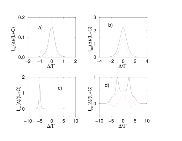
Figure 1: Backscattered light spectrum in the helicity-preserving polarization channel $h\parallel h$. The solid lines represent the ladder term (average background intensity value) and the dotted lines represent the crossed (interference) term. For both terms, the plotted values corresponds to $I_{\mathrm{inel}}(\Delta)/(C^{\mathrm{tot}}+L^{\mathrm{tot}})$, see Eq.(52), where $C^{\mathrm{tot}}+L^{\mathrm{tot}}$ is the total (elastic plus inelastic) intensity scattered in the backward direction. The vertical dashed lines indicate the atomic transition frequency. $\Delta$ corresponds to the scattered light angular frequency change with respect to the initial laser angular frequency ($\Delta=0$ means thus that light is radiated at $\omega_{L}$). Graph ($a$) corresponds to an on-resonance saturation parameter $s_{0}=0.02$ and a laser detuning $\delta=0$ ; Graph ($b$) to $(s_{0}=2,\delta=0)$ ; Graph ($c$) to $(s_{0}=2,\delta=5\Gamma)$ and Graph ($d$) to $(s_{0}=50,\delta=0)$. At low $s_{0}$, the inelastic contribution to the total intensity is small and the ladder intensity is almost equal to the crossed one. For a larger saturation parameter, firstly the inelastic contribution becomes comparable to the elastic one and secondly, the crossed term becomes smaller than the ladder one. For a nonzero detuning, see graph ($c$), one clearly observes an asymmetry in the inelastic spectrum, which reflects the fact that the scattering cross-section of the atomic transition is maximal for resonant light: the symmetric inelastic spectrum emitted by a single atom is filtered out when scattered by the other one. At very large saturation (d), the structure of the radiated spectrum becomes rather complicated.

The corresponding inelastic spectra $L_{\mathrm{inel}}(\Delta)$ and $C_{\mathrm{inel}}(\Delta)$ are displayed in figure 1. For a sufficiently low saturation parameter $s_{0}$, the inelastic contribution to the total intensity is small and the ladder intensity is almost equal to the crossed one (see graph 1$a$). For larger saturation parameters (see graphs 1$b$ and 1$d$), there are two effects : first, the inelastic contribution becomes comparable to the elastic one and second, the crossed term is smaller than the ladder one. For a nonzero detuning (see graph 1$c$), one clearly observes an asymmetry in the inelastic spectrum, which reflects that the scattering cross-section of the atomic transition is maximal for resonant light (indicated by the vertical dashed line): the symmetric inelastic spectrum emitted by a single atom is filtered out when scattered by the other one. We also observe that the crossed spectrum is much more reduced than the ladder term, highlighting the non-linear effects in the quantum correlations between the two atoms. Finally, for much larger saturation parameters (see graph 1$d$), the scattered light almost entirely originates from the inelastic spectrum, like for a single atom. However, contrary to the single atom case (for which the scattered intensity reaches a constant value), the total intensity scattered by the two atoms decreases when increasing the incoming intensity. Indeed, since the atomic transitions become fully saturated, the nonlinear scattering cross-section of each atom is decreasing, resulting in a smaller total intensity scattered by the two atoms compared to the one scattered by a single atom.

The CBS enhancement factor $\eta$ is defined as the peak to background ratio. It thus reads:

$$\eta=1+\frac{C^{\mathrm{tot}}}{L^{\mathrm{tot}}}$$ (53)

with:

$$L^{\mathrm{tot}} =L_{\mathrm{el}}+L_{\mathrm{inel}}^{\mathrm{tot}}=L_{\mathrm{el}}+\int\frac{d\Delta}{2\pi}\,L_{\mathrm{inel}}(\Delta)$$ (54)

$$C^{\mathrm{tot}} =C_{\mathrm{el}}+C_{\mathrm{inel}}^{\mathrm{tot}}=C_{\mathrm{el}}+\int\frac{d\Delta}{2\pi}\,C_{\mathrm{inel}}(\Delta)$$

If the CBS phenomenon is reducible to a two-wave interference, as it is the case here, then the enhancement factor $\eta$ is simply related to the degree of coherence $\gamma$ of the scattered light coherence . If the single scattering contribution can be removed from the detected signal, and this is the case in the $h\parallel h$ channel, one has simply $\eta=1+\gamma$ and consequently $\gamma=C^{\mathrm{tot}}/L^{\mathrm{tot}}$. The maximal value for $\eta$ is 2, meaning that full coherence $\gamma=1$ is maintained for the scattered field since then $C^{\mathrm{tot}}=L^{\mathrm{tot}}$. If all interference effects disappear, meaning $C^{\mathrm{tot}}=0$, $\eta$ reaches its minimal value 1 and correspondingly coherence is fully lost $\gamma=0$. Furthermore, one can show that in the $h\parallel h$ polarization channel, $L_{\mathrm{el}}=C_{\mathrm{el}}$ prl94SMB . Consequently, as soon as $C_{\mathrm{inel}}^{\mathrm{tot}}<L_{\mathrm{inel}}^{\mathrm{tot}}$ in this channel, the coherence of the scattered light field is partially destroyed, since then $\eta<2$ and $\gamma<1$.

Table 1: Ladder (average background) and crossed (interference) terms, see Eq.(52), contributing to the light scattered in the backward direction in the helicity-preserving polarization channel $h\parallel h$. The given values are relative to the incoming saturation parameter $s$. At low $s_{0}$, the inelastic contributions are small and almost equal. Thus $C^{\mathrm{tot}}\approx L^{\mathrm{tot}}$ and the maximum enhancement factor 2 of the linear case is thus recovered, meaning that full coherence $\gamma=1$ is maintained. At larger $s_{0}$, elastic and inelastic terms become comparable. For very large $s_{0}$, the contributions from the elastic terms vanish, like in the single atom case. The inelastic contributions are also decreasing, reflecting the fact that the probability for the light to be scattered by a saturated atom becomes smaller with increasing saturation. Furthermore, the inelastic crossed term is always smaller than the inelastic ladder one. This is a signature of a coherence loss $\gamma<1$ induced by the quantum vacuum fluctuations. However, the ratio $C_{\mathrm{inel}}^{\mathrm{tot}}/L_{\mathrm{inel}}^{\mathrm{tot}}$ does not go to zero as $s_{0}\to\infty$ but reaches the limit value 0.096 (for $\delta=0$). Also, contrary to the single atom case, the properties of the scattered light are not solely determined by the saturation parameter $s$, but additionally depend on the detuning $\delta,$ as exemplified by cases (a) and (c), highlighting the role of the inelastic processes.

	$(a)\,s=s_{0}=0.02,\delta=0$	$(b)\,s=s_{0}=2.00,\delta=0$	$(c)\,s=0.02,s_{0}=2.00,\delta=5\Gamma$	$(d)\,s=s_{0}=50.0,\delta=0$
$L_{\mathrm{el}}$	$0.624$	$0.833E-02$	$0.612$	$0.998E-07$
$L_{\mathrm{inel}}^{\mathrm{tot}}$	$0.220E-01$	$0.573E-01$	$0.328$	$0.487E-03$
$L^{\mathrm{tot}}$	$0.646$	$0.656E-01$	$0.946$	$0.487E-03$
$C_{\mathrm{el}}$	$0.624$	$0.833E-02$	$0.612$	$0.998E-07$
$C_{\mathrm{inel}}^{\mathrm{tot}}$	$0.188E-01$	$0.295E-01$	$0.157E-01$	$0.466E-04$
$C^{\mathrm{tot}}$	$0.642$	$0.378E-01$	$0.634$	$0.467E-04$
$\eta=1+\gamma$	$1.994$	$1.576$	$1.670$	$1.096$

Our results are summarized in table 1. At low saturation parameter $s_{0}$, $\eta$ reaches its maximal value 2 and $\gamma=1$. This is so because the ladder and crossed inelastic components are almost equal as evidenced in 1$a$. Increasing $s_{0}$ reduces further $C_{\mathrm{inel}}^{\mathrm{tot}}$ with respect to $L_{\mathrm{inel}}^{\mathrm{tot}}$, thus decreasing $\eta$ and $\gamma$. In the strongly saturated regime, one thus expects $\gamma$ to decrease. However, there is no reason for the ratio $C_{\mathrm{inel}}^{\mathrm{tot}}/L_{\mathrm{inel}}^{\mathrm{tot}}$ to tend to zero as $s_{0}\to\infty.$ It rather tends to a finite value, which depends on the detuning, in agreement with the results published in prl94SMB . Furthermore, keeping $s_{0}$ fixed and decreasing the saturation parameter $s$, situation $(c)$, $\eta$ increases, as expected, but to a value which strongly depends on $s_{0}$. In other words, contrary to the single atom case, the properties of the scattered light, are not only determined by the saturation parameter $s$ pra70WGDM . Indeed, in both situations $(a)$ and $(c)$, $s$ has the same (small) value, but the enhancement factor strongly differs, mainly because the inelastic ladder term has increased. This highlights the crucial role of the inelastic processes and of the rather complicated quantum correlations between the two atoms.

This is not however the full story. Depending on the $s$ and $\delta$ parameters, a rich variety of situations can be observed, with various physical interpretations. These are beyond the scope of this paper, which instead concentrates on the basic ingredients of the quantum Langevin approach and will be published elsewhere.

IV.3 Linear response model

Some insight on the relative behavior of $C_{\mathrm{inel}}(\Delta)$ and $L_{\mathrm{inel}}(\Delta)$ can be found by comparing the respective formulae from which these quantities are extracted:

$$\left\langle{X}_{i^{\prime}}^{\beta}[\Delta^{\prime}]{X}_{i}^{\alpha}[\Delta]\right\rangle^{(\bar{g}_{\beta}g_{\alpha})}=g_{\alpha}\left\langle{X}_{i^{\prime}}^{\beta^{(0)}}[\Delta^{\prime}]G_{ij}^{\alpha^{+}_{q}}[\Delta]\bigl{(}X_{j}^{\alpha^{(0)}}\otimes\mathcal{D}^{{\beta-}^{(0)}}_{q}\bigr{)}[\Delta]\right\rangle^{(\bar{g}_{\beta})}-\bar{g}_{\beta}\left\langle G_{i^{\prime}j^{\prime}}^{\beta^{-}_{q}}[\Delta^{\prime}]\bigl{(}\mathcal{D}^{{\alpha+}^{(0)}}_{q}\otimes X_{j^{\prime}}^{\beta^{(0)}}\bigr{)}[\Delta^{\prime}]{X}_{i}^{\alpha^{(0)}}[\Delta]\right\rangle^{(g_{{\alpha}})}\\ -g_{\alpha}\bar{g}_{\beta}\biggl{\{}\left\langle{X}_{i^{\prime}}^{\beta}[\Delta^{\prime}]G_{ij}^{\alpha^{+}_{q}}[\Delta]\left(X_{j}^{\alpha^{(0)}}\otimes G^{\beta^{-}_{p}}_{\mathcal{D}_{q}^{-}j^{\prime}}\left(\mathcal{D}^{{\alpha+}^{(0)}}_{p}\otimes X^{\beta^{(0)}}_{j^{\prime}}\right)\right)[\Delta]\right\rangle^{(0)}\\ +\left\langle G_{i^{\prime}j^{\prime}}^{\beta^{-}_{q}}[\Delta^{\prime}]\left(G^{\alpha^{+}_{p}}_{\mathcal{D}_{q}^{-}j}\left(X_{j}^{\alpha^{(0)}}\otimes\mathcal{D}^{{\beta-}^{(0)}}_{p}\right)\otimes X_{j^{\prime}}^{\beta^{(0)}}\right)[\Delta^{\prime}]{X}_{i}^{\alpha^{(0)}}[\Delta]\right\rangle^{(0)}\\ +\biggl{.}\left\langle\biggl{[}G_{i^{\prime}j^{\prime}}^{\beta^{-}_{p}}[\Delta^{\prime}]\bigl{(}\mathcal{D}^{{\alpha+}^{(0)}}_{p}\otimes X_{j^{\prime}}^{\beta^{(0)}}\bigr{)}[\Delta^{\prime}]\biggr{]}\biggl{[}G_{ij}^{\alpha^{+}_{q}}[\Delta]\bigl{(}X_{j}^{\alpha^{(0)}}\otimes\mathcal{D}^{{\beta-}^{(0)}}_{q}\bigr{)}[\Delta]\biggr{]}\right\rangle^{(0)}\biggr{\}}$$ (55)

and

$$\left\langle{X}_{i^{\prime}}^{\alpha}[\Delta^{\prime}]{X}_{i}^{\alpha}[\Delta]\right\rangle^{(\bar{g}_{\alpha}g_{\alpha})}=\left\langle{X}_{i^{\prime}}^{\alpha^{(0)}}[\Delta^{\prime}]{X}_{i}^{\alpha^{(0)}}[\Delta]\right\rangle^{(\bar{g}_{\alpha}g_{\alpha})}\\ +g_{\alpha}\biggl{\{}\left\langle{X}_{i^{\prime}}^{\alpha^{(0)}}[\Delta^{\prime}]G_{ij}^{\alpha^{+}_{q}}[\Delta]\bigl{(}X_{j}^{\alpha^{(0)}}\otimes\mathcal{D}^{{\beta-}^{(0)}}_{q}\bigr{)}[\Delta]\right\rangle^{(\bar{g}_{\alpha})}+\left\langle G_{i^{\prime}j^{\prime}}^{\alpha^{+}_{q}}[\Delta^{\prime}]\bigl{(}X_{j^{\prime}}^{\alpha^{(0)}}\otimes\mathcal{D}^{{\beta-}^{(0)}}_{q}\bigr{)}[\Delta^{\prime}]{X}_{i}^{\alpha^{(0)}}[\Delta]\right\rangle^{(\bar{g}_{\alpha})}\biggr{\}}\\ -\bar{g}_{\alpha}\biggl{\{}\left\langle{X}_{i^{\prime}}^{\alpha^{(0)}}[\Delta^{\prime}]G_{ij}^{\alpha^{-}_{q}}[\Delta]\bigl{(}\mathcal{D}^{{\beta+}^{(0)}}_{q}\otimes X_{j}^{\alpha^{(0)}}\bigr{)}[\Delta]\right\rangle^{(g_{\alpha})}+\left\langle G_{i^{\prime}j^{\prime}}^{\alpha^{-}_{q}}[\Delta^{\prime}]\bigl{(}\mathcal{D}^{{\beta+}^{(0)}}_{q}\otimes X_{j^{\prime}}^{\alpha^{(0)}}\bigr{)}[\Delta^{\prime}]{X}_{i}^{\alpha^{(0)}}[\Delta]\right\rangle^{(g_{\alpha})}\biggr{\}}\\ -\bar{g}_{\alpha}g_{\alpha}\biggl{\{}\left\langle{X}_{i^{\prime}}^{\alpha}[\Delta^{\prime}]G_{ij}^{\alpha^{+}_{q}}[\Delta]\left(G^{\alpha^{-}_{p}}_{jj^{\prime}}\left(\mathcal{D}^{{\beta+}^{(0)}}_{p}\otimes X_{j^{\prime}}^{\alpha^{(0)}}\right)\otimes\mathcal{D}^{{\beta-}^{(0)}}_{q}\right)[\Delta]\right\rangle^{(0)}\biggr{.}\\ +\left\langle{X}_{i^{\prime}}^{\alpha}[\Delta^{\prime}]G_{ij}^{\alpha^{-}_{q}}[\Delta]\left(\mathcal{D}^{{\beta+}^{(0)}}_{q}\otimes G^{\alpha^{+}_{p}}_{jj^{\prime}}\left(X_{j^{\prime}}^{\alpha^{(0)}}\otimes\mathcal{D}^{{\beta-}^{(0)}}_{p}\right)\right)[\Delta]\right\rangle^{(0)}\\ +\left\langle G_{i^{\prime}j^{\prime}}^{\alpha^{+}_{q}}[\Delta^{\prime}]\left(G^{\alpha^{-}_{p}}_{j^{\prime}j}\left(\mathcal{D}^{{\beta+}^{(0)}}_{p}\otimes X_{j}^{\alpha^{(0)}}\right)\otimes\mathcal{D}^{{\beta-}^{(0)}}_{q}\right)[\Delta^{\prime}]{X}_{i}^{\alpha^{(0)}}[\Delta]\right\rangle^{(0)}\\ +\left\langle G_{i^{\prime}j^{\prime}}^{\alpha^{-}_{q}}[\Delta^{\prime}]\left(\mathcal{D}^{{\beta+}^{(0)}}_{q}\otimes G^{\alpha^{+}_{p}}_{j^{\prime}j}\left(X_{j}^{\alpha^{(0)}}\otimes\mathcal{D}^{{\beta-}^{(0)}}_{p}\right)\right)[\Delta^{\prime}]{X}_{i}^{\alpha^{(0)}}[\Delta]\right\rangle^{(0)}\\ +\left\langle\biggl{[}G_{i^{\prime}j^{\prime}}^{\alpha^{+}_{p}}[\Delta^{\prime}]\bigl{(}X_{j^{\prime}}^{\alpha^{(0)}}\otimes\mathcal{D}^{{\beta-}^{(0)}}_{p}\bigr{)}[\Delta^{\prime}]\biggr{]}\biggl{[}G_{ij}^{\alpha^{-}_{q}}[\Delta]\bigl{(}\mathcal{D}^{{\beta+}^{(0)}}_{q}\otimes X_{j}^{\alpha^{(0)}}\bigr{)}[\Delta]\biggr{]}\right\rangle^{(0)}\\ +\biggl{.}\left\langle\biggl{[}G_{i^{\prime}j^{\prime}}^{\alpha^{-}_{p}}[\Delta^{\prime}]\bigl{(}\mathcal{D}^{{\beta+}^{(0)}}_{p}\otimes X_{j^{\prime}}^{{\alpha}^{(0)}}\bigr{)}[\Delta^{\prime}]\biggr{]}\biggl{[}G_{ij}^{\alpha^{+}_{q}}[\Delta]\bigl{(}X_{j}^{\alpha^{(0)}}\otimes\mathcal{D}^{{\beta-}^{(0)}}_{q}\bigr{)}[\Delta]\biggr{]}\right\rangle^{(0)}\biggr{\}}.$$ (56)

There are twice as many terms contributing to the ladder terms as to the crossed terms. A rather simple explanation of this fact is borrowed from the usual linear response theory. Indeed, each atom is exposed to two fields : the incoming monochromatic field (angular frequency $\omega_{L}$, wave vector $\textbf{k}_{L}$) and the field scattered by the other atom (angular frequency $\omega_{L}+\Delta$, wave vector $\textbf{k}_{p}$). In the far-field regime $R\gg\lambda$, the incoming field is more intense than the scattered field. It thus plays the role of a pump beam with angular Rabi frequency $\Omega_{L}$, while the second weaker field plays the role of a probe beam with angular Rabi frequency $\Omega_{p}$. In this case, the response of each atom is simply described by its nonlinear susceptibility Cohenrouge ; boyd . More precisely, forgetting about polarization effects, we have:

$$\delta\mathcal{D}^{+}[\Delta] =e^{-i(2\textbf{k}_{L}-\textbf{k}_{p})\cdot\textbf{R}_{\alpha}}\,\chi_{\scriptscriptstyle++}[\Delta]\,\Omega_{p}^{+}+e^{-i\textbf{k}_{p}\cdot\textbf{R}_{\alpha}}\,\chi_{\scriptscriptstyle+-}[\Delta]\,\Omega_{p}^{-}$$ (57)

$$\delta\mathcal{D}^{-}[\Delta] =e^{i\textbf{k}_{p}\cdot\textbf{R}_{\alpha}}\,\chi_{\scriptscriptstyle-+}[\Delta]\,\Omega_{p}^{+}+e^{i(2\textbf{k}_{L}-\textbf{k}_{p})\cdot\textbf{R}_{\alpha}}\,\chi_{\scriptscriptstyle--}[\Delta]\,\Omega_{p}^{-}.$$

where the phases due to the light fields have been explicitly factorized.

As obviously seen, the two terms $\chi_{\scriptscriptstyle+-}$ and $\chi_{\scriptscriptstyle-+}$ generate the forward propagation of the probe whereas the two other terms $\chi_{\scriptscriptstyle++}$ and $\chi_{\scriptscriptstyle--}$ can generate an additional field in the direction $2\textbf{k}_{L}-\textbf{k}_{p}$ provided phase-matching conditions are fulfilled. This corresponds to the usual forward four-wave mixing mechanism (FFWM) boyd ; Cohenrouge . If we now replace the probe field by the field radiated by the other atom $\beta$, we get:

$$\delta\mathcal{D}^{+}_{\beta\rightarrow\alpha}[\Delta] =\frac{1}{kR}\left\{e^{-i(kR+2\textbf{k}_{L}\cdot\textbf{R}_{\alpha}-\textbf{k}_{L}\cdot\textbf{R}_{\beta})}\chi_{\scriptscriptstyle++}[\Delta]\,\mathcal{D}^{-}_{\beta}+e^{i(kR-\textbf{k}_{L}\cdot\textbf{R}_{\beta})}\chi_{\scriptscriptstyle+-}[\Delta]\,\mathcal{D}^{+}_{\beta}\right\}$$ (58)

$$\delta\mathcal{D}^{-}_{\beta\rightarrow\alpha}[\Delta] =\frac{1}{kR}\left\{e^{-i(kR-\textbf{k}_{L}\cdot\textbf{R}_{\beta})}\chi_{\scriptscriptstyle-+}[\Delta]\,\mathcal{D}^{-}_{\beta}+e^{i(2\textbf{k}_{L}\cdot\textbf{R}_{\alpha}+kR-\textbf{k}_{L}\cdot\textbf{R}_{\beta})}\chi_{\scriptscriptstyle--}[\Delta]\,\mathcal{D}^{+}_{\beta}\right\}.$$

Hence the ladder and crossed contributions are given by (dropping for sake of clarity any frequency dependence):

$$C^{(2)} \approx\delta\mathcal{D}^{+}_{\alpha\rightarrow\beta}\delta\mathcal{D}^{-}_{\beta\rightarrow\alpha}e^{i(-\textbf{k}_{L}\cdot\textbf{R}_{\beta}+\textbf{k}_{L}\cdot\textbf{R}_{\alpha})}$$ (59)

$$\approx e^{i(2\textbf{k}_{L}\cdot(\textbf{R}_{\alpha}-\textbf{R}_{\beta})-2kR)}\chi_{\scriptscriptstyle++}\chi_{\scriptscriptstyle-+}\mathcal{D}^{-}_{\alpha}\mathcal{D}^{-}_{\beta}+e^{4i\textbf{k}_{L}\cdot(\textbf{R}_{\alpha}-\textbf{R}_{\beta})}\chi_{\scriptscriptstyle++}\chi_{\scriptscriptstyle--}\mathcal{D}^{-}_{\alpha}\mathcal{D}^{+}_{\beta}$$

$$\phantom{\approx}+\chi_{\scriptscriptstyle+-}\chi_{\scriptscriptstyle-+}\mathcal{D}^{+}_{\alpha}\mathcal{D}^{-}_{\beta}+e^{i(2\textbf{k}_{L}\cdot(\textbf{R}_{\alpha}-\textbf{R}_{\beta})+2kR)}\chi_{\scriptscriptstyle+-}\chi_{\scriptscriptstyle--}\mathcal{D}^{+}_{\alpha}\mathcal{D}^{+}_{\beta}$$

$$L^{(2)} \approx\delta\mathcal{D}^{+}_{\beta\rightarrow\alpha}\delta\mathcal{D}^{-}_{\beta\rightarrow\alpha}$$

$$\approx e^{i(2\textbf{k}_{L}\cdot(\textbf{R}_{\beta}-\textbf{R}_{\alpha})-2kR)}\chi_{\scriptscriptstyle++}\chi_{\scriptscriptstyle-+}\mathcal{D}^{-}_{\beta}\mathcal{D}^{-}_{\beta}+\chi_{\scriptscriptstyle++}\chi_{\scriptscriptstyle--}\mathcal{D}^{-}_{\beta}\mathcal{D}^{+}_{\beta}$$

$$\phantom{\approx}+\chi_{\scriptscriptstyle+-}\chi_{\scriptscriptstyle-+}\mathcal{D}^{+}_{\beta}\mathcal{D}^{-}_{\beta}+e^{i(2\textbf{k}_{L}\cdot(\textbf{R}_{\alpha}-\textbf{R}_{\beta})+2kR)}\chi_{\scriptscriptstyle+-}\chi_{\scriptscriptstyle--}\mathcal{D}^{+}_{\beta}\mathcal{D}^{+}_{\beta}.$$

Averaging these expressions over the positions $\textbf{R}_{\alpha}$ and $\textbf{R}_{\beta}$ of the atoms while keeping $R\gg\lambda$ fixed, only terms with position-independent phases survive, giving rise to:

$$C^{(2)} \approx\chi_{\scriptscriptstyle+-}\chi_{\scriptscriptstyle-+}\,\mathcal{D}^{+}_{\alpha}\mathcal{D}^{-}_{\beta}$$ (60)

$$L^{(2)} \approx\chi_{\scriptscriptstyle++}\chi_{\scriptscriptstyle--}\,\mathcal{D}^{-}_{\beta}\mathcal{D}^{+}_{\beta}+\chi_{\scriptscriptstyle+-}\chi_{\scriptscriptstyle-+}\,\mathcal{D}^{+}_{\beta}\mathcal{D}^{-}_{\beta}.$$

This simple model allows to understand clearly why there are twice more terms in the ladder expression than in the crossed one. Fields generated in the FFWM process always interfere constructively in the case of the ladder, since they originate from the same atom. Of course, in the preceding explanation, we have discarded polarization effects and inelastic processes in the nonlinear susceptibilities. Nevertheless, even if in that case the situation becomes more involved, the differences between the ladder and crossed expressions still arise from this local four wave-mixing process. For example, in the last line of Eqs. (55) and (56), we see that the operator $\big{(}G_{ij}^{\alpha^{+}_{q}}[\Delta]X_{j}^{\alpha^{(0)}}\otimes\big{)}$ plays the role of a generalized nonlinear susceptibility (actually, the standard ones are recovered from the elastic part of $X_{j}^{\alpha^{(0)}}$). Thus we recover the same structure as previously depicted, which leads to similar conclusions.

Finally, as mentioned above, for large saturation parameters $s_{0}$, even if in that case the total scattered intensities (ladder and crossed) are dominated by the inelastic spectrum, we numerically observe that the enhancement factor does not vanish but rather goes to a finite limit $1.096$ (for $\delta=0$). Field coherence is thus not fully erased, which, at first glance, could be surprising since the inelastic spectrum is a noise spectrum at the heart of the temporal decoherence of the radiated field. But this only means that both crossed and ladder become vanishingly small relatively to the incident intensity. Nevertheless, even if it would be hard to derive it analytically from Eqs. (55) and (56), they actually decrease at the same rate, resulting in a finite (but small) enhancement factor.

V Conclusion

In the case of two atoms, even if the quantum Langevin approach leads to calculations more tedious and involved than the direct optical Bloch method, it nevertheless gives rise to an understanding closer to the usual scattering approach developed in the linear regime. In this way, one also gets direct information about the inelastic spectrum of the radiated light. In particular, it clearly outlines the crucial roles played by the inelastic nonlinear susceptibilities and by the quantum correlations of the vacuum fluctuations. Furthermore, since the framework of the quantum Langevin approach is set in the frequency domain, frequency-dependent propagation (i.e. frequency-dependent mean-free paths) between the atoms can be naturally included.

The next step would be to adapt the present approach to ”macroscopic” configurations (i.e. at least many atoms), allowing for a more direct comparison with existing experiments thierry . This would provide a better understanding of light transport properties in nonlinear atomic media where vacuum fluctuations play a role. In particular, for given values of the incident laser intensity and detuning, the nonlinear mean-free path becomes negative in well-defined frequency windows. This means that light amplification can be achieved in these frequency windows pra5M ; prl38WEDM . The atomic media would then constitute a very simple realization of a coherent random laser.

Appendix A

The $g\bar{g}$ terms in Eq. (31) read:

$${X}_{i^{\prime}}^{\beta}[\Delta^{\prime}]{X}_{i}^{\alpha}[\Delta]=\cdots\\ -g\bar{g}\biggl{\{}{X}_{i^{\prime}}^{\beta}[\Delta^{\prime}]\biggl{[}G_{ij}^{\alpha^{+}_{q}}[\Delta]\left(X_{j}^{\alpha^{(0)}}\otimes G^{\beta^{-}_{p}}_{\mathcal{D}_{q}^{-}j^{\prime}}\left(\mathcal{D}^{{\alpha+}^{(0)}}_{p}\otimes X^{\beta^{(0)}}_{j^{\prime}}\right)\right)[\Delta]+G_{ij}^{\alpha^{+}_{q}}[\Delta]\left(G^{\alpha^{-}_{p}}_{jj^{\prime}}\left(\mathcal{D}^{{\beta+}^{(0)}}_{p}\otimes X_{j^{\prime}}^{\alpha^{(0)}}\right)\otimes\mathcal{D}^{{\beta-}^{(0)}}_{q}\right)[\Delta]\biggr{.}\biggr{.}\\ \biggl{.}+G_{ij}^{\alpha^{-}_{q}}[\Delta]\left(\mathcal{D}^{{\beta+}^{(0)}}_{q}\otimes G^{\alpha^{+}_{p}}_{jj^{\prime}}\left(X_{j^{\prime}}^{\alpha^{(0)}}\otimes\mathcal{D}^{{\beta-}^{(0)}}_{p}\right)\right)[\Delta]+G_{ij}^{\alpha^{-}_{q}}[\Delta]\left(G^{\beta^{+}_{p}}_{\mathcal{D}_{q}^{-}j^{\prime}}\left(X_{j^{\prime}}^{\beta^{(0)}}\otimes\mathcal{D}^{{\alpha-}^{(0)}}_{p}\right)\otimes X_{j}^{\alpha^{(0)}}\right)[\Delta]\biggr{]}\\ \biggl{[}G_{i^{\prime}j^{\prime}}^{\beta^{+}_{q}}[\Delta^{\prime}]\left(X_{j^{\prime}}^{\beta^{(0)}}\otimes G^{\alpha^{-}_{p}}_{\mathcal{D}_{q}^{-}j}\left(\mathcal{D}^{{\beta+}^{(0)}}_{p}\otimes X^{\alpha^{(0)}}_{j}\right)\right)[\Delta^{\prime}]+G_{i^{\prime}j^{\prime}}^{\beta^{+}_{q}}[\Delta^{\prime}]\left(G^{\beta^{-}_{p}}_{j^{\prime}j}\left(\mathcal{D}^{{\alpha+}^{(0)}}_{p}\otimes X_{j}^{\beta^{(0)}}\right)\otimes\mathcal{D}^{{\alpha-}^{(0)}}_{q}\right)[\Delta^{\prime}]\biggr{.}\\ \biggl{.}+G_{i^{\prime}j^{\prime}}^{\beta^{-}_{q}}[\Delta^{\prime}]\left(\mathcal{D}^{{\alpha+}^{(0)}}_{q}\otimes G^{\beta^{+}_{p}}_{j^{\prime}j}\left(X_{j}^{\beta^{(0)}}\otimes\mathcal{D}^{{\alpha-}^{(0)}}_{p}\right)\right)[\Delta^{\prime}]+G_{i^{\prime}j^{\prime}}^{\beta^{-}_{q}}[\Delta^{\prime}]\left(G^{\alpha^{+}_{p}}_{\mathcal{D}_{q}^{-}j}\left(X_{j}^{\alpha^{(0)}}\otimes\mathcal{D}^{{\beta-}^{(0)}}_{p}\right)\otimes X_{j^{\prime}}^{\beta^{(0)}}\right)[\Delta^{\prime}]\biggr{]}{X}_{i}^{\alpha^{(0)}}[\Delta]\\ +\biggl{[}G_{i^{\prime}j^{\prime}}^{\beta^{+}_{p}}[\Delta^{\prime}]\biggl{(}X_{j^{\prime}}^{\beta^{(0)}}\otimes\mathcal{D}^{{\alpha-}^{(0)}}_{p}\biggr{)}[\Delta^{\prime}]\biggr{]}\biggl{[}G_{ij}^{\alpha^{-}_{q}}[\Delta]\biggl{(}\mathcal{D}^{{\beta+}^{(0)}}_{q}\otimes X_{j}^{\alpha^{(0)}}\biggr{)}[\Delta]\biggr{]}\\ +\biggl{.}\biggl{[}G_{i^{\prime}j^{\prime}}^{\beta^{-}_{p}}[\Delta^{\prime}]\biggl{(}\mathcal{D}^{{\alpha+}^{(0)}}_{p}\otimes X_{j^{\prime}}^{\beta^{(0)}}\biggr{)}[\Delta^{\prime}]\biggr{]}\biggl{[}G_{ij}^{\alpha^{+}_{q}}[\Delta]\biggl{(}X_{j}^{\alpha^{(0)}}\otimes\mathcal{D}^{{\beta-}^{(0)}}_{q}\biggr{)}[\Delta]\biggr{]}\biggr{\}}$$ (61)

$${X}_{i^{\prime}}^{\alpha}[\Delta^{\prime}]{X}_{i}^{\alpha}[\Delta]=\cdots\\ -g\bar{g}\biggl{\{}{X}_{i^{\prime}}^{\alpha}[\Delta^{\prime}]\biggl{[}G_{ij}^{\alpha^{+}_{q}}[\Delta]\left(X_{j}^{\alpha^{(0)}}\otimes G^{\beta^{-}_{p}}_{\mathcal{D}_{q}^{-}j^{\prime}}\left(\mathcal{D}^{{\alpha+}^{(0)}}_{p}\otimes X^{\beta^{(0)}}_{j^{\prime}}\right)\right)[\Delta]+G_{ij}^{\alpha^{+}_{q}}[\Delta]\left(G^{\alpha^{-}_{p}}_{jj^{\prime}}\left(\mathcal{D}^{{\beta+}^{(0)}}_{p}\otimes X_{j^{\prime}}^{\alpha^{(0)}}\right)\otimes\mathcal{D}^{{\beta-}^{(0)}}_{q}\right)[\Delta]\biggr{.}\biggr{.}\\ \biggl{.}+G_{ij}^{\alpha^{-}_{q}}[\Delta]\left(\mathcal{D}^{{\beta+}^{(0)}}_{q}\otimes G^{\alpha^{+}_{p}}_{jj^{\prime}}\left(X_{j^{\prime}}^{\alpha^{(0)}}\otimes\mathcal{D}^{{\beta-}^{(0)}}_{p}\right)\right)[\Delta]+G_{ij}^{\alpha^{-}_{q}}[\Delta]\left(G^{\beta^{+}_{p}}_{\mathcal{D}_{q}^{-}j^{\prime}}\left(X_{j^{\prime}}^{\beta^{(0)}}\otimes\mathcal{D}^{{\alpha-}^{(0)}}_{p}\right)\otimes X_{j}^{\alpha^{(0)}}\right)[\Delta]\biggr{]}\\ \biggl{[}G_{i^{\prime}j^{\prime}}^{\alpha^{+}_{q}}[\Delta^{\prime}]\left(X_{j^{\prime}}^{\alpha^{(0)}}\otimes G^{\beta^{-}_{p}}_{\mathcal{D}_{q}^{-}j}\left(\mathcal{D}^{{\alpha+}^{(0)}}_{p}\otimes X^{\beta^{(0)}}_{j}\right)\right)[\Delta^{\prime}]+G_{i^{\prime}j^{\prime}}^{\alpha^{+}_{q}}[\Delta^{\prime}]\left(G^{\alpha^{-}_{p}}_{j^{\prime}j}\left(\mathcal{D}^{{\beta+}^{(0)}}_{p}\otimes X_{j}^{\alpha^{(0)}}\right)\otimes\mathcal{D}^{{\beta-}^{(0)}}_{q}\right)[\Delta^{\prime}]\biggr{.}\\ \biggl{.}+G_{i^{\prime}j^{\prime}}^{\alpha^{-}_{q}}[\Delta^{\prime}]\left(\mathcal{D}^{{\beta+}^{(0)}}_{q}\otimes G^{\alpha^{+}_{p}}_{j^{\prime}j}\left(X_{j}^{\alpha^{(0)}}\otimes\mathcal{D}^{{\beta-}^{(0)}}_{p}\right)\right)[\Delta^{\prime}]+G_{i^{\prime}j^{\prime}}^{\alpha^{-}_{q}}[\Delta^{\prime}]\left(G^{\beta^{+}_{p}}_{\mathcal{D}_{q}^{-}j}\left(X_{j}^{\beta^{(0)}}\otimes\mathcal{D}^{{\alpha-}^{(0)}}_{p}\right)\otimes X_{j^{\prime}}^{\alpha^{(0)}}\right)[\Delta^{\prime}]\biggr{]}{X}_{i}^{\alpha^{(0)}}[\Delta]\\ +\biggl{[}G_{i^{\prime}j^{\prime}}^{\alpha^{+}_{p}}[\Delta^{\prime}]\biggl{(}X_{j^{\prime}}^{\alpha^{(0)}}\otimes\mathcal{D}^{{\beta-}^{(0)}}_{p}\biggr{)}[\Delta^{\prime}]\biggr{]}\biggl{[}G_{ij}^{\alpha^{-}_{q}}[\Delta]\biggl{(}\mathcal{D}^{{\beta+}^{(0)}}_{q}\otimes X_{j}^{\alpha^{(0)}}\biggr{)}[\Delta]\biggr{]}\\ +\biggl{.}\biggl{[}G_{i^{\prime}j^{\prime}}^{\alpha^{-}_{p}}[\Delta^{\prime}]\biggl{(}\mathcal{D}^{{\beta+}^{(0)}}_{p}\otimes X_{j^{\prime}}^{{\alpha}^{(0)}}\biggr{)}[\Delta^{\prime}]\biggr{]}\biggl{[}G_{ij}^{\alpha^{+}_{q}}[\Delta]\biggl{(}X_{j}^{\alpha^{(0)}}\otimes\mathcal{D}^{{\beta-}^{(0)}}_{q}\biggr{)}[\Delta]\biggr{]}\biggr{\}}$$ (62)

Appendix B Three-body correlation functions

B.1 Single atom case

The three-body correlation function for the Langevin force reads:

$$C_{abc}[\Delta^{\prime},\Delta]=\frac{1}{2\pi}\iint d\Delta_{1}d\Delta_{2}\delta[\Delta_{1}+\Delta_{2}-\Delta]f[\Delta_{1}]g[\Delta_{2}]\left\langle F^{{\alpha}}_{a}[\Delta^{\prime}]F^{{\alpha}}_{b}[\Delta_{1}]F^{{\alpha}}_{c}[\Delta_{2}]\right\rangle,$$ (63)

where $f[\Delta]$ and $g[\Delta]$ are regular functions such that the preceding integral is well defined. Going back to the time domain, $C_{abc}[\Delta^{\prime},\Delta]$ reads as follows:

$$C_{abc}[\Delta^{\prime},\Delta]=\frac{1}{2\pi}\iint dtdt^{\prime}e^{i\Delta t}e^{i\Delta^{\prime}t^{\prime}}\iiiint dt_{1}dt_{2}dt_{3}dt_{4}\delta(t_{1}+t_{2}-t)\delta(t_{3}+t_{4}-t)f(t_{1})g(t_{3})\left\langle F^{{\alpha}}_{a}(t^{\prime})F^{{\alpha}}_{b}(t_{2})F^{{\alpha}}_{c}(t_{4})\right\rangle.$$ (64)

Then, from the time correlation properties of the vacuum field, one can show that:

$$\left\langle F^{{\alpha}}_{a}(t^{\prime})F^{{\alpha}}_{b}(t_{2})F^{{\alpha}}_{c}(t_{4})\right\rangle =4T^{q+}_{aa^{\prime}}T^{q-}_{bb^{\prime}}\delta(t^{\prime}-t_{2})\left\langle X^{{\alpha}}_{a^{\prime}}(t^{\prime})X^{{\alpha}}_{b^{\prime}}(t^{\prime})F^{{\alpha}}_{c}(t_{4})\right\rangle$$ (65)

$$+4T^{q+}_{aa^{\prime}}T^{q-}_{cc^{\prime}}\delta(t^{\prime}-t_{4})\left\langle X^{{\alpha}}_{a^{\prime}}(t^{\prime})F^{{\alpha}}_{b}(t_{2})X^{{\alpha}}_{c^{\prime}}(t_{4})\right\rangle$$

$$+4T^{q+}_{bb^{\prime}}T^{q-}_{cc^{\prime}}\delta(t_{2}-t_{4})\left\langle F^{{\alpha}}_{a}(t^{\prime})X^{{\alpha}}_{b^{\prime}}(t_{2})X^{{\alpha}}_{c^{\prime}}(t_{2})\right\rangle.$$

where the $T^{q\pm}$ are $15\times 15$ matrices defined by $\left[X_{i},\mathcal{D}^{\pm}_{q}\right]=\pm 2T^{q\pm}_{ij}X_{j}$.

When taken at the same time, the atomic operators (including the identity $\openone$) define a group entirely characterized by the group structure constants $\epsilon_{ij}^{\phantom{ij}k}$, i.e.:

$$X_{i}(t)X_{j}(t)=\sum_{k}\epsilon_{ij}^{\phantom{ij}k}X_{k}(t),$$ (66)

so that the preceding equation becomes:

$$\left\langle F^{{\alpha}}_{a}(t^{\prime})F^{{\alpha}}_{b}(t_{2})F^{{\alpha}}_{c}(t_{4})\right\rangle =4T^{q+}_{aa^{\prime}}T^{q-}_{bb^{\prime}}\delta(t^{\prime}-t_{2})\epsilon_{a^{\prime}b^{\prime}}^{\phantom{a^{\prime}b^{\prime}}u}\left\langle X^{{\alpha}}_{u}(t^{\prime})F^{{\alpha}}_{c}(t_{4})\right\rangle$$ (67)

$$+4T^{q+}_{aa^{\prime}}T^{q-}_{cc^{\prime}}\delta(t^{\prime}-t_{4})\left\langle X^{{\alpha}}_{a^{\prime}}(t^{\prime})F^{{\alpha}}_{b}(t_{2})X^{{\alpha}}_{c^{\prime}}(t_{4})\right\rangle$$

$$+4T^{q+}_{bb^{\prime}}T^{q-}_{cc^{\prime}}\delta(t_{2}-t_{4})\epsilon_{a^{\prime}b^{\prime}}^{\phantom{b^{\prime}c^{\prime}}u}\left\langle F^{{\alpha}}_{a}(t^{\prime})X^{{\alpha}}_{u}(t_{2})\right\rangle.$$

Injecting the preceding relations in $C(a,b,c)$ and going back to the frequency domain, we get:

$$C_{abc}[\Delta^{\prime},\Delta] =4T^{q+}_{aa^{\prime}}T^{q-}_{bb^{\prime}}\epsilon_{a^{\prime}b^{\prime}}^{\phantom{a^{\prime}b^{\prime}}u}\frac{1}{2\pi}\iint d\Delta_{1}d\Delta_{2}\delta(\Delta_{1}+\Delta_{2}-\Delta)f[\Delta_{1}]g[\Delta_{2}]\left\langle X^{{\alpha}}_{u}[\Delta^{\prime}+\Delta_{1}]F^{{\alpha}}_{c}[\Delta_{2}]\right\rangle$$ (68)

$$\phantom{=}+4T^{q+}_{aa^{\prime}}T^{q-}_{cc^{\prime}}\frac{1}{2\pi}\int d\Delta_{3}g[\Delta_{3}]f[\Delta-\Delta_{3}]D^{b,\alpha\alpha\alpha}_{a^{\prime}c^{\prime}}[\Delta^{\prime}+\Delta_{3},\Delta-\Delta_{3}]$$

$$\phantom{=}+4T^{q+}_{bb^{\prime}}T^{q-}_{cc^{\prime}}\epsilon_{a^{\prime}b^{\prime}}^{\phantom{b^{\prime}c^{\prime}}u}\left\langle F^{{\alpha}}_{a}[\Delta^{\prime}]X^{{\alpha}}_{u}[\Delta]\right\rangle\frac{1}{2\pi}\iint d\Delta_{1}d\Delta_{2}\delta(\Delta_{1}+\Delta_{2}-\Delta)f[\Delta_{1}]g[\Delta_{2}]$$

$$=4T^{q+}_{aa^{\prime}}T^{q-}_{bb^{\prime}}\epsilon_{a^{\prime}b^{\prime}}^{\phantom{a^{\prime}b^{\prime}}u}\frac{1}{2\pi}\iint d\Delta_{1}d\Delta_{2}\delta(\Delta_{1}+\Delta_{2}-\Delta)f[\Delta_{1}]g[\Delta_{2}]G^{\alpha}_{uv}[\Delta^{\prime}+\Delta_{1}]\left\langle F^{{\alpha}}_{v}[\Delta^{\prime}+\Delta_{1}]F^{{\alpha}}_{c}[\Delta_{2}][\right\rangle$$

$$\phantom{=}+4T^{q+}_{aa^{\prime}}T^{q-}_{cc^{\prime}}\frac{1}{2\pi}\int d\Delta_{3}g[\Delta_{3}]f[\Delta-\Delta_{3}]D^{b,\alpha\alpha\alpha}_{a^{\prime}c^{\prime}}[\Delta^{\prime}+\Delta_{3},\Delta-\Delta_{3}]$$

$$\phantom{=}+4T^{q+}_{bb^{\prime}}T^{q-}_{cc^{\prime}}\epsilon_{a^{\prime}b^{\prime}}^{\phantom{b^{\prime}c^{\prime}}u}G_{uv}^{\alpha}[\Delta]\left\langle F^{{\alpha}}_{a}[\Delta^{\prime}]F^{{\alpha}}_{v}[\Delta]\right\rangle\frac{1}{2\pi}\iint d\Delta_{1}d\Delta_{2}\delta(\Delta_{1}+\Delta_{2}-\Delta)f[\Delta_{1}]g[\Delta_{2}]$$

$$=2\pi\delta[\Delta+\Delta^{\prime}]4T^{q+}_{aa^{\prime}}T^{q-}_{bb^{\prime}}\epsilon_{a^{\prime}b^{\prime}}^{\phantom{a^{\prime}b^{\prime}}u}D^{\alpha\alpha}_{vc}\frac{1}{2\pi}\iint d\Delta_{1}d\Delta_{2}\delta(\Delta_{1}+\Delta_{2}-\Delta)f[\Delta_{1}]g[\Delta_{2}]G^{\alpha}_{uv}[-\Delta_{2}]$$

$$\phantom{=}+4T^{q+}_{aa^{\prime}}T^{q-}_{cc^{\prime}}\frac{1}{2\pi}\int d\Delta_{3}g[\Delta_{3}]f[\Delta-\Delta_{3}]D^{b,\alpha\alpha\alpha}_{a^{\prime}c^{\prime}}[\Delta^{\prime}+\Delta_{3},\Delta-\Delta_{3}]$$

$$\phantom{=}+2\pi\delta[\Delta+\Delta^{\prime}]4T^{q+}_{bb^{\prime}}T^{q-}_{cc^{\prime}}\epsilon_{a^{\prime}b^{\prime}}^{\phantom{b^{\prime}c^{\prime}}u}D^{\alpha\alpha}_{av}G_{uv}^{\alpha}[\Delta]\frac{1}{2\pi}\iint d\Delta_{1}d\Delta_{2}\delta(\Delta_{1}+\Delta_{2}-\Delta)f[\Delta_{1}]g[\Delta_{2}],$$

where we have introduced the matrix $D^{b,\alpha\alpha\alpha}_{ik}[\Delta^{\prime},\Delta]$ defined by:

$$D^{b,\alpha\alpha\alpha}_{ik}[\Delta^{\prime},\Delta]=\frac{1}{2\pi}\iint d\Delta_{1}d\Delta_{2}\delta(\Delta_{1}+\Delta_{2}-\Delta^{\prime})\left\langle X^{{\alpha}}_{i}[\Delta_{1}]F^{{\alpha}}_{b}[\Delta]X^{{\alpha}}_{k}[\Delta_{2}]\right\rangle.$$ (69)

This matrix is calculated using the same strategy (i.e. going back and forth to the time domain) and one finally gets:

$$D^{b,\alpha\alpha\alpha}_{ik}[\Delta^{\prime},\Delta]=2\pi\delta[\Delta+\Delta^{\prime}]\left\{G^{\alpha}_{ia}[0]L^{\alpha}_{a}G^{\alpha}_{kc}[\Delta^{\prime}]\tilde{D}^{\alpha\alpha}_{bc}+G^{\alpha}_{ia}[\Delta^{\prime}]G^{\alpha}_{kc}[0]L^{\alpha}_{c}\tilde{D}^{\alpha\alpha}_{ab}\right.\\ \left.+4T^{q+}_{bb^{\prime}}T^{q-}_{cc^{\prime}}\epsilon_{b^{\prime}c^{\prime}}^{\phantom{b^{\prime}c^{\prime}}v}\tilde{D}^{\alpha\alpha}_{au}\frac{1}{2\pi}\iint d\Delta_{1}d\Delta_{2}\delta(\Delta_{1}+\Delta_{2}-\Delta^{\prime})G^{\alpha}_{ia}[\Delta_{1}]G^{\alpha}_{kc}[\Delta_{2}]G^{\alpha}_{vu}[-\Delta_{1}]\right.\\ \left.+4T^{+}_{aa^{\prime}}T^{-}_{bb^{\prime}}\epsilon_{a^{\prime}b^{\prime}}^{\phantom{a^{\prime}b^{\prime}}v}\tilde{D}^{\alpha\alpha}_{uc}\frac{1}{2\pi}\iint d\Delta_{1}d\Delta_{2}\delta(\Delta_{1}+\Delta_{2}-\Delta^{\prime})G^{\alpha}_{ia}[\Delta_{1}]G^{\alpha}_{kc}[\Delta_{2}]G^{\alpha}_{vu}[-\Delta_{2}]\right\}\\ +4T^{q+}_{aa^{\prime}}T^{q-}_{cc^{\prime}}\left(\frac{1}{2\pi}\iint d\Delta_{3}d\Delta_{4}\delta(\Delta_{3}+\Delta_{4}-\Delta^{\prime})G^{\alpha}_{ia}[\Delta_{3}]G^{\alpha}_{kc}[\Delta_{4}]\right)\\ \times\left(\frac{1}{2\pi}\iint d\Delta_{1}d\Delta_{2}\delta(\Delta_{1}+\Delta_{2}-\Delta^{\prime})\left\langle X^{{\alpha}}_{a^{\prime}}[\Delta_{1}]F^{{\alpha}}_{b}[\Delta]X^{{\alpha}}_{c^{\prime}}[\Delta_{2}]\right\rangle\right).$$ (70)

It may seem that we have taken a loop path and that we are back to square one… However, in the last line of the preceding formula, we immediately recognize the matrix $D^{b,\alpha\alpha\alpha}_{a^{\prime}b^{\prime}}[\Delta^{\prime},\Delta]$. Thus, the preceding equation is nothing else but a linear system for this matrix. More precisely, $D^{b,\alpha\alpha\alpha}_{ik}[\Delta^{\prime},\Delta]$ is the solution of the following linear system:

$$D_{ik}^{b,\alpha\alpha\alpha}[\Delta^{\prime},\Delta]-I_{ik,a^{\prime}c^{\prime}}^{\alpha\alpha}[\Delta^{\prime}]D_{a^{\prime}c^{\prime}}^{b,\alpha\alpha\alpha}[\Delta^{\prime},\Delta]=J_{ik}^{b,\alpha\alpha\alpha}[\Delta^{\prime},\Delta],$$ (71)

with

$$\left\{\begin{aligned} I_{ik,a^{\prime}c^{\prime}}^{\alpha\alpha}[\Delta^{\prime}]&=4T^{q+}_{aa^{\prime}}T^{q-}_{cc^{\prime}}\frac{1}{2\pi}\iint d\Delta_{3}d\Delta_{4}\delta(\Delta_{3}+\Delta_{4}-\Delta^{\prime})G^{\alpha}_{ia}[\Delta_{3}]G^{\alpha}_{kc}[\Delta_{4}]\\ J_{ik}^{b,\alpha\alpha\alpha}[\Delta^{\prime},\Delta]&=2\pi\delta[\Delta+\Delta^{\prime}]\left\{G^{\alpha}_{ia}[0]L^{\alpha}_{a}G^{\alpha}_{kc}[\Delta^{\prime}]\tilde{D}^{\alpha\alpha}_{bc}+G^{\alpha}_{ia}[\Delta^{\prime}]G^{\alpha}_{kc}[0]L^{\alpha}_{c}\tilde{D}^{\alpha\alpha}_{ab}\right.\\ &\phantom{=2\pi\delta[\Delta+\Delta^{\prime}]}\quad\left.+4T^{q+}_{bb^{\prime}}T^{q-}_{cc^{\prime}}\epsilon_{b^{\prime}c^{\prime}}^{\phantom{b^{\prime}c^{\prime}}v}\tilde{D}^{\alpha\alpha}_{au}\frac{1}{2\pi}\iint d\Delta_{1}d\Delta_{2}\delta(\Delta_{1}+\Delta_{2}-\Delta^{\prime})G^{\alpha}_{ia}[\Delta_{1}]G^{\alpha}_{kc}[\Delta_{2}]G^{\alpha}_{vu}[-\Delta_{1}]\right.\\ &\phantom{=2\pi\delta[\Delta+\Delta^{\prime}]}\quad\left.+4T^{+}_{aa^{\prime}}T^{-}_{bb^{\prime}}\epsilon_{a^{\prime}b^{\prime}}^{\phantom{a^{\prime}b^{\prime}}v}\tilde{D}^{\alpha\alpha}_{uc}\frac{1}{2\pi}\iint d\Delta_{1}d\Delta_{2}\delta(\Delta_{1}+\Delta_{2}-\Delta^{\prime})G^{\alpha}_{ia}[\Delta_{1}]G^{\alpha}_{kc}[\Delta_{2}]G^{\alpha}_{vu}[-\Delta_{2}]\right\}\end{aligned}\right..$$ (72)

In the preceding equations, the Green’s function $G[\Delta]$ and the diffusion matrix $D^{\alpha\alpha}$ only depend on the Rabi field $\Omega_{L}$ evaluated at the position of atom $\alpha$. Thus, for any value of $\Delta$, numerical values of $I$ and $J$ can be computed, allowing for a direct calculation of $D_{ik}^{b,\alpha\alpha\alpha}[-\Delta,\Delta]$. Furthermore, it is not surprising that the matrix $I$ shows up in the linear system. Indeed, the Green’s function $G[\Delta]$ governs the time evolution of X through a Fourier transform. Thus the time evolution of products of operators $\textbf{X}_{i}(t)\textbf{X}_{j}(t)$ will be simply governed by the Fourier transform of the product of two Green’s functions $G(t)G(t)$, which is precisely the convolution product found in $I$. Finally, from the knowledge of the matrix $D$, we can calculate the value of $C_{abc}[\Delta^{\prime},\Delta]$:

$$C_{abc}[\Delta^{\prime},\Delta] =2\pi\delta[\Delta+\Delta^{\prime}]\left\{4T^{q+}_{aa^{\prime}}T^{q-}_{bb^{\prime}}\epsilon_{a^{\prime}b^{\prime}}^{\phantom{a^{\prime}b^{\prime}}u}D^{\alpha\alpha}_{vc}\frac{1}{2\pi}\iint d\Delta_{1}d\Delta_{2}\delta(\Delta_{1}+\Delta_{2}-\Delta)f[\Delta_{1}]g[\Delta_{2}]G^{\alpha}_{uv}[-\Delta_{2}]\right.$$ (73)

$$\phantom{=2\pi\delta[\Delta+\Delta^{\prime}]}\quad+4T^{q+}_{aa^{\prime}}T^{q-}_{cc^{\prime}}\frac{1}{2\pi}\iint d\Delta_{1}d\Delta_{2}\delta(\Delta_{1}+\Delta_{2}-\Delta)f[\Delta_{1}]g[\Delta_{2}]D^{b,\alpha\alpha\alpha}_{a^{\prime}c^{\prime}}[-\Delta_{1},\Delta_{1}]$$

$$\phantom{=2\pi\delta[\Delta+\Delta^{\prime}]}\quad+\left.4T^{q+}_{bb^{\prime}}T^{q-}_{cc^{\prime}}\epsilon_{a^{\prime}b^{\prime}}^{\phantom{b^{\prime}c^{\prime}}u}D^{\alpha\alpha}_{av}G_{uv}^{\alpha}[\Delta]\frac{1}{2\pi}\iint d\Delta_{1}d\Delta_{2}\delta(\Delta_{1}+\Delta_{2}-\Delta)f[\Delta_{1}]g[\Delta_{2}]\right\}.$$

Of course, we recover the global factor $2\pi\delta[\Delta+\Delta^{\prime}]$, showing that the time correlation function only depends on the time difference $t^{\prime}-t$ (stationary condition).

B.2 Two-atom case

The calculation of quantities like:

$$C^{\alpha\beta}_{abc}[\Delta^{\prime},\Delta]=\frac{1}{2\pi}\iint d\Delta_{1}d\Delta_{2}\delta[\Delta_{1}+\Delta_{2}-\Delta]f[\Delta_{1}]g[\Delta_{2}]\left\langle F^{\alpha}_{j^{\prime}}[\Delta^{\prime}]F^{\beta}_{k}[\Delta_{1}]F^{{\alpha}}_{k^{\prime}}[\Delta_{2}]\right\rangle^{(\bar{g})},$$ (74)

follows, more or less, the way described in the preceding section. In particular, it also involves the calculation of a matrix $D^{b,{\alpha}\beta\alpha^{(\bar{g})}}_{ik}[\Delta^{\prime},\Delta]$ defined as follows:

$$D^{b,{\alpha}\beta\alpha^{(\bar{g})}}_{ik}[\Delta^{\prime},\Delta]=\frac{1}{2\pi}\iint d\Delta_{1}d\Delta_{2}\delta(\Delta_{1}+\Delta_{2}-\Delta^{\prime})\left\langle X^{{\alpha}}_{i}[\Delta_{1}]F^{\beta}_{b}[\Delta]X^{{\alpha}}_{k}[\Delta_{2}]\right\rangle^{(\bar{g})}.$$ (75)

The latter is also found to be the solution of a linear system, resembling the preceding one (see Eq. (71)):

$$D_{ik}^{b,{\alpha}\beta\alpha^{(\bar{g})}}[\Delta^{\prime},\Delta]-I_{ik,a^{\prime}c^{\prime}}^{{\alpha}{\alpha}}[\Delta^{\prime}]D_{a^{\prime}c^{\prime}}^{b,{\alpha}\beta\alpha^{(\bar{g})}}[\Delta^{\prime},\Delta]=J_{ik}^{b,{\alpha}\beta\alpha^{(\bar{g})}}[\Delta^{\prime},\Delta],$$ (76)

with

$$J_{ik}^{b,\alpha\beta\alpha^{(\bar{g})}}[\Delta^{\prime},\Delta]=-\left(\frac{1}{2}\right)2\pi\delta[\Delta+\Delta^{\prime}]\biggl{\{}G^{\alpha}_{ia}[0]L^{\alpha}_{a}G^{\alpha}_{kc}[\Delta^{\prime}]\tilde{D}^{\beta\alpha^{(0)}}_{bc}+G^{\alpha}_{ia}[\Delta^{\prime}]G^{\alpha}_{kc}[0]L^{\alpha}_{c}\tilde{D}^{\alpha\beta^{(0)}}_{ab}\biggr{.}\\ +4T^{q+}_{bb^{\prime}}\langle X^{\beta^{(0)}}_{b^{\prime}}\rangle\frac{1}{2\pi}\iint d\Delta_{1}d\Delta_{2}\delta(\Delta_{1}+\Delta_{2}-\Delta^{\prime})G^{\alpha}_{ia}[\Delta_{1}]G^{\alpha^{-}_{q}}_{kc}[\Delta_{2}]G^{\alpha}_{cu}[-\Delta_{1}]\tilde{D}^{\alpha\alpha^{(0)}}_{au}\\ +4T^{q-}_{bb^{\prime}}\langle X^{\beta^{(0)}}_{b^{\prime}}\rangle\frac{1}{2\pi}\iint d\Delta_{1}d\Delta_{2}\delta(\Delta_{1}+\Delta_{2}-\Delta^{\prime})G^{\alpha^{+}_{q}}_{ia}[\Delta_{1}]G^{\alpha}_{kc}[\Delta_{2}]G^{\alpha}_{au}[-\Delta_{2}]\tilde{D}^{\alpha\alpha^{(0)}}_{uc}\\ -2G^{\beta}_{\mathcal{D}^{+}_{q}u}[\Delta^{\prime}]\tilde{D}^{\beta\beta^{(0)}}_{ub}\frac{1}{2\pi}\iint d\Delta_{1}d\Delta_{2}\delta(\Delta_{1}+\Delta_{2}-\Delta^{\prime})G^{\alpha^{-}_{q}}_{ia}[\Delta_{1}]\langle\tilde{X}^{\alpha^{(0)}}_{a}[-\Delta_{2}]\tilde{X}^{\alpha^{(0)}}_{k}[\Delta_{2}]\rangle^{(0)}\\ \biggl{.}-2G^{\beta}_{\mathcal{D}^{+}_{q}u}[\Delta^{\prime}]\tilde{D}^{\beta\beta^{(0)}}_{bu}\frac{1}{2\pi}\iint d\Delta_{1}d\Delta_{2}\delta(\Delta_{1}+\Delta_{2}-\Delta^{\prime})G^{\alpha^{-}_{q}}_{kc}[\Delta_{2}]\langle\tilde{X}^{\alpha^{(0)}}_{i}[\Delta_{1}]\tilde{X}^{\alpha^{(0)}}_{c}[-\Delta_{1}]\rangle^{(0)}\biggr{\}}.$$ (77)

References

- (1) C. J. Pethick and H. Smith, Bose-Einstein Condensation in Dilute Gases (Cambridge University Press, Cambridge, 2002); L. P. Pitaevskii and S. Stringari, Bose-Einstein Condensation (Clarendon Press, Oxford, 2003).
- (2) M. Greiner, C. A. Regal, and D. S Jin, Nature (London) 426, 537 (2003); S. Jochim et al., Science 302, 2101 (2003).
- (3) M. Greiner, O. Mandel, T. Esslinger, T.W. Hänsch, and I. Bloch, Nature 415, 39-44 (2002).
- (4) W. K. Hensinger et al., Phys. Rev. A 70, 013408 (2004); Z.Y. Ma, M.B. d’Arcy, and S.A. Gardiner, Phys. Rev. Lett. 93, 164101 (2004).
- (5) R. Battesti et al., Phys. Rev. Lett. 92, 253001 (2004); M. Weitz, B.C. Young, and S. Chu, Phys. Rev. Lett. 73, 2563 (1994).
- (6) G. Labeyrie et al., Phys. Rev. Lett. 83, 5266 (1999).
- (7) T. Chanelière, D. Wilkowski, Y. Bidel, R. Kaiser and C. Miniatura, Phys. Rev. E 70, 036602 (2004).
- (8) Mesoscopic quantum physics, Proceedings of the Les Houches Summer School, Session LXI, E. Akkermans and G. Montambaux and J. L. Pichard and J. Zinn-Justin eds, North Holland, Elsevier Science B. V., Amsterdam (1995).
- (9) Physique mésoscopique des électrons et des photons, E. Akkermans and G. Montambaux, EDP Sciences, CNRS Editions (2004). An english translation is in preparation.
- (10) M. P. Van Albada and A. Lagendijk, Phys. Rev. Lett. 55, 2692 (1985); P. E. Wolf and G. Maret, Phys. Rev. Lett. 55, 2696 (1985).
- (11) A. Akkermans and G. Montambaux, J. Opt. Soc. Am. B 21, 101 (2004).
- (12) D. Wilkowski et al., J. Opt. Soc. Am. B 21, 183 (2004) and references therein.
- (13) O. Sigwarth et al., Phys. Rev. Lett. 93, 143906 (2004).
- (14) C.A. Müller, T. Jonckheere, C. Miniatura and D. Delande, Phys. Rev. A 64, 053804 (2001).
- (15) R. W. Boyd, Nonlinear Optics, (Academic, San Diego, 1992).
- (16) G. Grynberg, A. Maître, and A. Petrossian Phys. Rev. Lett. 72, 2379-2382 (1994)
- (17) M. L. Dowell, R. C. Hart, A. Gallagher, and J. Cooper Phys. Rev. A 53, 1775 (1996)
- (18) S. E. Skipetrov and R. Maynard Phys. Rev. Lett. 85, 736 (2000)
- (19) T. Wellens, B. Grémaud, D. Delande, and C. Miniatura, Phys. Rev. A 70, 023817 (2004).
- (20) T. Wellens, B. Grémaud, D. Delande, and C. Miniatura, Phys. Rev. E In press (2005).
- (21) T. Wellen et al, in preparation.
- (22) C. Cohen-Tannoudji, J. Dupont-Roc, and G. Grynberg, Atom-Photon Interactions (Wiley, New York, 1992).
- (23) B.R. Mollow, Phys. Rev. 188, 1969 (1969).
- (24) C.W. Gardiner and P. Zoller, Quantum Noise 2nd ed, (Springer, Berlin Heidelberg, 1999).
- (25) L. You, J. Mostowski, and J. Cooper, Phys. Rev. A 46, 2903 (1992).
- (26) L. You, J. Mostowski, and J. Cooper, Phys. Rev. A 46, 2925 (1992).
- (27) L. You, and J. Cooper, Phys. Rev. A 51, 4194 (1995)
- (28) M.L. Dowell, B.D. Paul, A. Gallagher, and J. Cooper, Phys. Rev. A 52, 3244 (1995).
- (29) Y. Ben-Aryeh, Phys. Rev. A 56, 854 (1997).
- (30) H. Cao, Waves Random Media 13, R1 (2003).
- (31) G. V. Varada and G. S. Agarwal Phys. Rev. A 45, 6721-6729 (1992).
- (32) V. Shatokhin, C. A. Müller, and A. Buchleitner Phys. Rev. Lett. 94, 043603 (2005).
- (33) C. Cohen-Tannoudji, J. Dupont-Roc, and G. Grynberg, Photons and Atoms, Introduction to Quantum Electrodynamics (Wiley, New York, 1989).
- (34) J.M. Courty and S. Reynaud, Phys. Rev. A 46, 2766 (1992).
- (35) B.R. Mollow, Phys. Rev. A 5, 2217 (1972).
- (36) B. van Tiggelen and R. Maynard, in Waves in Random and other complex media, L. Burridge, G. Papanicolaou and L. Pastur eds., Springer, vol. 96, p247 (1997).
- (37) Please note however that this result is no longer true as soon as inelastic scattering occurs in a medium : in this case, CBS can arise from a three-wave interference facteur3 .
- (38) F.Y. Wu, S. Ezekiel, M. Ducloy and B.R. Mollow, Phys. Rev. Lett. 38, 1077 (1977).
- (39) G. Labeyrie, E. Vaujour, C. A. Müller, D. Delande, C. Miniatura, D. Wilkowski and R. Kaiser, Phys. Rev. Lett., 91, 223904 (2003).