Phase Control of Trapped Ion Quantum Gates

Abstract

There are several known schemes for entangling trapped ion quantum bits for large-scale quantum computation. Most are based on an interaction between the ions and external optical fields, coupling internal qubit states of trapped-ions to their Coulomb-coupled motion. In this paper, we examine the sensitivity of these motional gate schemes to phase fluctuations introduced through noisy external control fields, and suggest techniques to suppress the resulting phase decoherence.

Scalable quantum computing presents a direct application for the study and control of large-scale quantum systems. The generally accepted requirements for quantum hardware [1] include identifiable two-level-systems for storing information in the form of quantum bits (or qubits), and methods to externally manipulate and entangle qubits through quantum logic gate operations. The implicit interconnects represented by entangled quantum systems provide the power behind quantum computation, giving rise to certain applications such as Shor’s factoring algorithm [2] and Grover’s search algorithm [3] that exceed the capabilities of classical computers. However, in engineering complex entangled states of many qubits, it is critical to control the phase of the system of qubits and the phase of the classical control parameters that guide the quantum gates. Techniques of quantum error-correction [4, 5] appear essential to stabilize quantum computations, but to reach fault-tolerant error-correction thresholds [6], the host system must already possess a great deal of passive stability and must be relatively insensitive to external noise.

One of the most promising quantum computing architectures is a system of cold atomic ions confined in free space with electromagnetic fields [7, 8, 9]. Here, qubits are stored in stable electronic states of each ion, and quantum information can be processed and transferred through the collective quantized motion of the Coulomb-coupled ion crystal. Applied electromagnetic fields (usually from a laser) enable this coupling between internal qubit states and external motional states, following several known quantum gate schemes [7, 10, 11, 12]. Trapped ion quantum gates are thus highly susceptible to noise on the applied laser fields in addition to ambient electric and magnetic fields. In most cases, the relevant phases of the laser fields for quantum gates can be sufficiently stable during the evolution of a given gate, with gate speeds typically faster than about $100\mu s$. However, for extended operations involving many successive gates, it will be difficult to maintain optical phase stability over the duration of the quantum computation.

From an engineering standpoint, the ability to perform gate operations on any individual qubit or set of qubits with a given phase at any step in a series of operations is requisite to a universal quantum computer. We assume that all operations are synchronized to a local oscillator in perfect resonance with the qubits. Each qubit initially has an arbitrarily defined phase, and subsequent phase accumulations from interactions must be tracked so that each operation account for the phase of the individual qubit. These interactions are primarily AC Stark shifts from the optical control fields [13] and Zeeman shifts from ambient magnetic fields. Our goal here is to prescribe a set of gates that leave the qubits independent of the optical phase of the driving field after each operation is complete while enjoying passive isolation from Stark and Zeeman qubit phase shifts.

In this paper, we consider several quantum gate schemes in the trapped ion system, concentrating on a class of currently-favored quantum gates that rely on a “spin-dependent force” [14, 10, 15, 11, 16, 12, 17], and are relatively insensitive to motional heating from noisy background electric fields [18, 19]. We will discuss the sources of phase decoherence for these gates and describe methods to suppress decoherence from slow phase drifts of the driving optical fields. We find that certain gate schemes can be simultaneously insensitive to background magnetic fields, making them quite robust for long-term computations.

This paper is divided into three sections: Section 1 lays out the background for the various quantum gate schemes for trapped ion system, covering detailed steps for performing single qubit operations and a discussion of the original Cirac-Zoller model with special attention paid to the phases of the qubits [7]. Section 2 describes entangling gates using a spin-dependent force. We show how special arrangements of the classical driving fields can suppress slow phase decoherence from laser noise and external magnetic field noise [17]. Section 3 shows how to similarly suppress long-term phase noise in a recent “fast” gate scheme that relies on impulsive spin-dependent optical forces [12].

1 Background

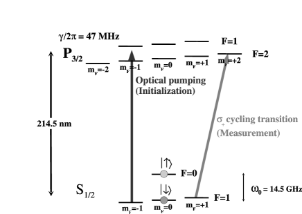
Figure 1: ¹¹¹Cd⁺ as an example of a hyperfine qubit. The ${}^{2}S_{1/2}$ ground state electron configuration combined with the nuclear spin $I=1/2$ creates an energy splitting of 14.5GHz due to the hyperfine interaction. The states $\left|F=0,m_{F}=0\right\rangle$ and $\left|F=1,m_{F}=0\right\rangle$ are called “clock” states at zero magnetic field since their energy difference has no first order dependence on the magnetic field, and are designated as the qubit states $\left|\uparrow\right\rangle$ and $\left|\downarrow\right\rangle$ respectively. A small external magnetic field lifts the degeneracy of the $F=1$ states through the Zeeman effect. Due to the large ground state hyperfine splitting, the qubit can be initialized by optically pumping into the $\left|\uparrow\right\rangle=\left|F=0,m_{F}=0\right\rangle$ state. The qubit state can be measured by applying resonant $\sigma_{+}$ radiation to optically pump the $\left|\downarrow\right\rangle=\left|F=1,m_{F}=0\right\rangle$ state to the $\left|F=1,m_{F}=1\right\rangle$ state and drive a cycling transition between the ${}^{2}S_{1/2}$, $F=1$ and the ${}^{2}P_{3/2}$, $F=2$ excited state and collecting the resulting fluorescence.

Typical atomic ion species for quantum information applications such as ⁹Be⁺, ⁴³Ca⁺, and ¹¹¹Cd⁺ have a single valence electron with a ${}^{2}S_{1/2}$ ground state and ${}^{2}P_{J}$ first excited electronic states. In isotopes with nonzero nuclear spin, the ${}^{2}S_{1/2}$ ground states are split by the hyperfine interaction. An applied static magnetic field $\mathbf{B}_{0}$ provides a quantization axis and removes degeneracy in the ground state Zeeman levels. Two states, one from each ground state hyperfine level, are designated as the qubit states, denoted by $\uparrow_{i}$ and $\downarrow_{i}$ for each ion $i$ and separated by energy $E_{\uparrow}-E_{\downarrow}=\hbar\omega_{0}$. At certain values of $\mathbf{B}_{0}$, this energy splitting can be insensitive to magnetic field fluctuations to first order, forming a qubit that can have particularly good phase stability. Such qubit levels are termed “clock states” because their stability is exploited in atomic clocks [20]. The qubit frequency splitting $\omega_{0}$ is usually in the microwave range and large compared with the radiative line-width $\gamma$ of excited electronic states, therefore the qubit can be measured with high fidelity by resonant pumping to a cycling transition between one hyperfine state and an excited electronic state [8]. Initialization of the qubits can also be accomplished with high accuracy using optical pumping techniques (Figure 1).

We assume ions are confined in a linear Paul trap [21] with a combination of static and radio frequency (rf) electric quadrupole potentials [22]. When the ions are sufficiently cold, their Coulomb repulsion balances the external confinement forces, and the ions form stationary crystals with the residual motion described by coupled harmonic oscillatory motion in the trap. The number of collective modes scales linearly with the number of atoms $N$ in the trap, making it difficult to isolate and control all modes of oscillation for large numbers of ions. To circumvent this difficulty, an architecture has been proposed for shuttling ions between multiple trap regions in a trap structure such that it is only necessary to localize a small number of ions at a given time [9]. Two-qubit quantum gates in addition to arbitrary single qubit rotations are sufficient for the engineering of arbitrarily complex entangled states [1], so we focus on the operation of quantum gates on $N=2$ ions, although extensions to larger numbers of ions is straightforward.

The ions arrange themselves along the weakest ($x$) axis of the confinement potential, and the position operator of each ion can be written as $\hat{\mathbf{R}}_{i}=\mathbf{R}_{0,i}+\hat{\mathbf{r}}_{i}$, with the operator $\hat{\mathbf{r}}_{i}$ describing the small quantum harmonic oscillations of each ion about its equilibrium position $\mathbf{R}_{0,i}$. Of the six normal modes of oscillation for the two ions, only the two axial normal modes will be considered for simplicity (see section 1.1): the center-of-mass coordinate $\hat{q}_{1}=(\hat{x}_{1}+\hat{x}_{2})/\sqrt{2}$ and a “stretch” coordinate $\hat{q}_{2}=(\hat{x}_{1}-\hat{x}_{2})/\sqrt{2}$, where $\hat{x}_{i}$ is the component of $\hat{\mathbf{r}}_{i}$ along the $x$-axis. The base Hamiltonian for the collective system is

$$\hat{H}_{0}=\sum_{i=1,2}\hbar\omega_{0}\left|\uparrow_{i}\right\rangle\left\langle\uparrow_{i}\right|+\sum_{\nu=1,2}\hbar\omega_{\nu}\hat{a}_{\nu}^{\dagger}\hat{a}_{\nu}$$ (1)

where $\omega_{0}$ is the frequency difference between the two qubit states; $\omega_{1}$ and $\omega_{2}=\sqrt{3}\omega_{1}$ are the frequencies associated with the center-of-mass and stretch modes, respectively; and $\hat{a}_{\nu}^{\dagger}$ and $\hat{a}_{\nu}$ are their respective harmonic oscillator creation and annihilation operators. The first term in the Hamiltonian describes the internal energy of the ions, and the second term describes the external vibrational energy of the system.

Single qubit rotations between hyperfine qubit levels (not involving ion motion) can be performed by applying appropriate radiation fields. For example, a resonant microwave field can directly couple the qubit levels through a magnetic dipole interaction, resulting in coherent Rabi oscillations between the two qubit states. Alternatively, optical stimulated-Raman transitions can be employed [23], using two optical sources that coherently couple the qubit states through excited ${}^{2}P_{J}$ electronic states, as discussed next.

1.1 Coherent Interaction between Trapped-Ion Hyperfine Qubits and Optical Fields

An optical coupling between the hyperfine qubit states and an excited electronic state of each ion can be exploited to entangle qubit states with collective motional states, forming the backbone of most trapped ion quantum logic gates. As shown in Figure 2, we assume each of two trapped ions consists of three levels: the two ground state qubit levels $\left|\uparrow_{i}\right\rangle$ and $\left|\downarrow_{i}\right\rangle$ and an excited electronic state $\left|e_{i}\right\rangle$ having respective optical frequency spans $\tilde{\omega}_{\uparrow,e}$ and $\tilde{\omega}_{\downarrow,e}=\tilde{\omega}_{\uparrow,e}+\omega_{0}$. Two optical fields $\mathbf{E}_{l}(\mathbf{r})=\tilde{E}_{l}(\mathbf{r})\cos(\mathbf{k}_{l}\mbox{$\cdot$}\mathbf{r}-\omega_{l}t-\phi_{l})\mbox{\boldmath$\epsilon$}_{l}$ with $l=\alpha,\beta$ and polarization $\mbox{\boldmath$\epsilon$}_{l}$, connect each of the qubit levels $\left|\uparrow_{i}\right\rangle$ and $\left|\downarrow_{i}\right\rangle$, respectively, to state $\left|e_{i}\right\rangle$ through electric dipole operators $\mbox{\boldmath$\mu$}_{\uparrow}$ and $\mbox{\boldmath$\mu$}_{\downarrow}$. We assume that the optical fields have a difference frequency $\omega_{\beta}-\omega_{\alpha}=\omega_{0}+\delta\omega$ and are both detuned from the excited-state resonance by $\Delta=\tilde{\omega}_{\uparrow,e}-\omega_{\alpha}$, as drawn in Figure 2. These fields evaluated at the ion’s position $\mathbf{E}_{l}(\hat{\mathbf{R}}_{i})$ are what ultimately couples the spin to the motion.

The interaction can be transformed to a rotating frame at frequency $\omega_{\alpha}$ in order to remove all terms varying with optical frequencies, and under the usual optical rotating wave approximation (RWA), the interaction Hamiltonian between the fields and the ions is

$$\hat{H}_{I}=\frac{\hbar}{2}\sum_{i=1,2}\bigg{[}-\left(g_{\uparrow,\alpha,i}e^{i\mathbf{k}_{\alpha}\cdot\hat{\mathbf{R}}_{i}-i\phi_{\alpha}}\left|e_{i}\right\rangle\left\langle\downarrow_{i}\right|+h.c.\right)-\left(g_{\downarrow,\beta,i}e^{i\mathbf{k}_{\beta}\cdot\hat{\mathbf{R}}_{i}-i\phi_{\beta}}e^{-i(\delta\omega)t}\left|e_{i}\right\rangle\left\langle\uparrow_{i}\right|+h.c.\right)$$

$$\hbox to0.0pt{\hss${}+{}$}\Delta\left|e_{i}\right\rangle\left\langle e_{i}\right|\bigg{]}$$ (2)

In this expression, the dipole coupling strengths between qubit state $\left|m_{i}\right\rangle=\left|\uparrow_{i}\right\rangle,\left|\downarrow_{i}\right\rangle$ and excited state $\left|e_{i}\right\rangle$ from laser field $l$ on ion $i$ are given by $\hbar g_{m,l,i}=-$$\mbox{\boldmath$\mu$}_{m}\cdot\mbox{\boldmath$\epsilon$}_{l}\tilde{E}_{l}(\mathbf{R}_{0,i})$$/2$.

For most of the remainder of this paper (outside of Section 3), we assume that the detuning $\Delta$ of the optical fields from electronic resonance is much larger than the excited state line-width $\gamma$ and the couplings $\left|g_{m,l,i}\right|^{2}$, so that spontaneous emission during the optical coupling is negligible [8] and the excited state $\left|e_{i}\right\rangle$ can be adiabatically eliminated. Applying RWA on the microwave frequencies, we find

$$\hat{H}_{I}=-\frac{\hbar}{2}\sum_{i=1,2}\bigg{[}\left(\Omega_{i}e^{-i(\Delta\mathbf{k}\cdot\mathbf{\hat{R}}_{i}-(\delta\omega)t-\Delta\phi)}\left|\uparrow_{i}\right\rangle\left\langle\downarrow_{i}\right|+h.c.\right)$$

$$\hbox to0.0pt{\hss${}+{}$}\chi_{\downarrow,i}\left|\downarrow_{i}\right\rangle\left\langle\downarrow_{i}\right|+\chi_{\uparrow,i}\left|\uparrow_{i}\right\rangle\left\langle\uparrow_{i}\right|\bigg{]}$$ (3)

where $\Delta\mathbf{k}=\mathbf{k}_{\beta}-\mathbf{k}_{\alpha}$ and $\Delta\phi=\phi_{\beta}-\phi_{\alpha}$ are the differences in the wave-vector and the phase of the two applied fields, $\Omega_{i}=g_{\uparrow,\alpha,i}g_{\downarrow,\beta,i}^{*}/2\Delta$ is the “base Rabi frequency” directly coupling the qubit states of ion $i$, and $\chi_{m,i}=\left(\left|g_{m,\alpha,i}\right|^{2}+\left|g_{m,\beta,i}\right|^{2}\right)/2$ corresponds to the AC Stark shifts of the qubit level $\left|m_{i}\right\rangle$ of ion $i$ by both optical fields.

For simplicity, we assume $\Delta\mathbf{k}$ is parallel to the x-axis ($\Delta k=\left|\Delta\mathbf{k}\right|$), so that the interaction deals only with axial motion (although it is straightforward to treat the more general case). We substitute the x-component of the position operator $\hat{\mathbf{R}}_{i}$ for ion $i$ by

$$\hat{X}_{i}=X_{0,i}+\frac{q_{1}}{\sqrt{2}}(\hat{a}_{1}+\hat{a}_{1}^{\dagger})\pm\frac{q_{2}}{\sqrt{2}}(\hat{a}_{2}+\hat{a}_{2}^{\dagger})$$ (4)

where $q_{\nu}=\sqrt{\hbar/(2M\omega_{\nu})}$ is the root mean square spatial spread of the ground state wavepacket for normal mode $\nu$ of oscillation in the trap, $M$ is the single ion mass, and the plus (minus) sign refers to ion $i=1$ ($i=2)$. In the interaction frame of the vibrational levels, Equation 3 becomes

$$\hat{H}_{I}=-\frac{\hbar}{2}\sum_{i=1,2}\bigg{[}(\Omega_{i}e^{-i\left[\eta_{1}(\hat{a}_{1}e^{-i\omega_{1}t}+\hat{a}_{1}^{\dagger}e^{i\omega_{1}t})\pm\eta_{2}(\hat{a}_{2}e^{-i\omega_{2}t}+\hat{a}_{2}^{\dagger}e^{i\omega_{2}t})\right]}e^{i(\delta\omega)t}e^{-i(\Delta kX_{0,i}-\Delta\phi)}\left|\uparrow_{i}\right\rangle\left\langle\downarrow_{i}\right|+h.c.)$$

$$\hbox to0.0pt{\hss${}+{}$}\chi_{\beta,i}\left|\downarrow_{i}\right\rangle\left\langle\downarrow_{i}\right|+\chi_{\alpha,i}\left|\uparrow_{i}\right\rangle\left\langle\uparrow_{i}\right|\bigg{]}$$ (5)

The Lamb-Dicke parameters are defined by $\eta_{1}=\Delta kq_{1}/\sqrt{2}$ and $\eta_{2}=\Delta kq_{2}/\sqrt{2}=\eta_{1}/\sqrt[4]{3}$, representing the coupling strength between the fields and each normal mode.

The above treatment can be generalized to the case of multiple optical sources that connect both qubit states to any number of excited states, resulting in higher order expressions for $\Omega_{i}$ and $\chi_{m,i}$. Here however, we are mainly interested in the sensitivity of entangling gate operations on the optical phases $\phi_{l}$. The net optical phase appearing in the coupling Hamiltonian (Equation 3) is sensitive only to the phase difference $\Delta\phi=\phi_{\beta}-\phi_{\alpha}$ between the two optical fields, so that when both fields are generated from a single laser and modulator, fluctuations in the optical phase of the laser source become common mode and do not lead to decoherence [24]. However, in order to couple the qubits with the motion for entangling quantum gates, the optical sources are generally non-copropagating ($\Delta k$$\neq 0$), opening up the sensitivity to decoherence from fluctuations in relative beam path lengths or ions’ positions through the phase factor $e^{i\Delta kX_{0,i}-i\Delta\phi}$. This requires interferometric stability between the optical paths of the fields $E_{\alpha}$ and $E_{\beta}$, which should be feasible over short times using stable optical mounts and indexing the laser beams to the trap structure itself. However, over the long time scale represented by an extended quantum computation, drifts in the phase $e^{i\Delta kX_{0,i}-i\Delta\phi}$ can be a serious source of decoherence.

1.2 Resolved-Sideband Limit

Equation 3 includes direct couplings between qubit states, and entangling couplings between qubit states and trapped ion motional states. We consider the case where the base Rabi frequencies $\Omega_{i}$ are much smaller than the vibrational frequencies $\omega_{\nu}$ of the ions in the trap. In this case, the difference frequency $\delta\omega$ of the optical sources can be tuned to particular values so that a single stationary term emerges from the above Hamiltonian, and all others couplings can be neglected under the rotating wave approximation. In this regime, as seen from the rest frame of the ions, the applied laser fields acquire resolved frequency-modulation sidebands from the ions’ harmonic vibration. We concentrate on three spectral features: the “carrier”, the first upper and lower sidebands, each selected by appropriate tuning of the radiation field difference frequency.

1.2.1 The carrier

When the difference frequency between the optical sources is tuned to the free-ion qubit resonance (compensating for possible differential Stark shifts, assumed to be equal for the two ions), then $\omega_{\beta}-\omega_{\alpha}=\omega_{0}+\chi_{\uparrow,i}-\chi_{\downarrow,i}\equiv\omega_{0}^{\prime}$ (Figure 3a ), and we find the stationary term in Equation 3 is given by [8]

$$\hat{H}_{I}^{car}=-\frac{\hbar}{2}\sum_{i=1,2}\sum_{n_{1},n_{2}}\left(\Omega_{i}\mathcal{D}_{n_{1},n_{2}}e^{i(\Delta kX_{0,i}-\Delta\phi)}\hat{\sigma}_{+}^{(i)}+h.c.\right)\left|n_{1},n_{2}\right\rangle\left\langle n_{1},n_{2}\right|.$$ (6)

This “carrier” interaction describes simple Rabi flopping between the qubit states in each ion, where the qubit raising and lowering operators are defined by $\hat{\sigma}_{+}^{(i)}=\left|\uparrow_{i}\right\rangle\left\langle\downarrow_{i}\right|$ and $\hat{\sigma}_{-}^{(i)}=(\hat{\sigma}_{+}^{(i)})^{\dagger}=\left|\downarrow_{i}\right\rangle\left\langle\uparrow_{i}\right|$. Also, $\mathcal{D}_{n_{1},n_{2}}=e^{-\frac{1}{2}(\eta_{1}^{2}+\eta_{2}^{2})}\mathcal{L}_{n_{1}}(\eta_{1}^{2})\mathcal{L}_{n_{2}}(\eta_{2}^{2})$ is the Debye-Waller factor that exponentially suppresses the carrier coupling due to ion motion described by vibrational quantum numbers $n_{\nu}$ in each mode $\nu$ of motion, with $\mathcal{L}_{n_{\nu}}(z)$ being a Laguerre polynomial of order $n_{\nu}$ [8]. When the ions are confined to the Lamb-Dicke limit (LDL) where $\eta_{\nu}^{2}(n_{\nu}+1/2)\ll 1$, then $\mathcal{D}_{n_{1},n_{2}}\simeq 1$. However, if the motion of either mode is not in a pure eigenstate of harmonic motion and outside of the LDL, then the Rabi frequency will depend upon the noisy motional quantum state and lead to qubit decoherence. In order to avoid this problem, carrier operations are often performed with copropagating Raman beams ($\eta_{\nu}=0$) thereby forcing $\mathcal{D}_{n_{1},n_{2}}=1$. A carrier transition using a copropagating geometry can also be insensitive to the phase noise of the source laser, making it ideal for single qubit rotations.

1.2.2 The first lower (red) sideband

When the difference frequency between the optical sources is tuned lower than the free-atom qubit resonance by the vibrational frequency $\omega_{\nu}$ of mode $\nu$ (again compensating for differential Stark shifts), $\omega_{\beta}-\omega_{\alpha}=\omega_{0}^{\prime}-\omega_{\nu}$ (Figure 3b) and we find the stationary term in Equation 3 is [8]

$$\mathcal{\hat{H}}_{I}^{rsb}=-\frac{\hbar}{2}\sum_{i=1,2}\left(\eta_{\nu}\Omega_{i}e^{i(\Delta kX_{0,i}-\Delta\phi)}\mathcal{D}_{n_{\nu},n_{\nu^{\prime}}}^{\prime}\hat{\sigma}_{+}^{(i)}\hat{a}_{\nu}+h.c.\right).$$ (7)

This “red sideband“ interaction describes Rabi flopping between the coupled qubit-motional states $\left|\downarrow,n_{\nu}\right\rangle$ and $\left|\uparrow,n_{\nu}-1\right\rangle$ in each ion, where $\mathcal{D}_{n_{\nu},n_{\nu^{\prime}}}^{\prime}=e^{-\frac{1}{2}(\eta_{1}^{2}+\eta_{2}^{2})}\frac{\mathcal{L}_{n_{\nu}-1}^{1}(\eta_{\nu}^{2})}{n_{\nu-1}!}\mathcal{L}_{n_{\nu^{\prime}}}(\eta_{\nu^{\prime}}^{2})$ is the Debye-Waller factor for the first sideband, with $\nu^{\prime}\neq\nu$ the “spectator” mode of motion. Here, $\mathcal{L}_{n}^{1}(z)$ is an associated Laguerre polynomial. This interaction is the Jaynes-Cummings Hamiltonian [25] where energy is exchanged between the internal qubit and the external harmonic oscillator states.

1.2.3 The first upper (blue) sideband

When the difference frequency between the optical sources is tuned higher than the free-atom qubit resonance by the vibrational frequency $\omega_{\nu}$ of mode $\nu$ (once again compensating for differential Stark shifts), $\omega_{\beta}-\omega_{\alpha}=\omega_{0}^{\prime}+\omega_{\nu}$ (Figure 3c) and we find the stationary term in Equation 3 is now [8]

$$\mathcal{\hat{H}}_{I}^{bsb}=-\frac{\hbar}{2}\sum_{i=1,2}\left(\eta_{\nu}\Omega_{i}e^{i(\Delta kX_{0,i}-\Delta\phi)}\mathcal{D}_{n_{\nu},n_{\nu^{\prime}}}^{\prime}\hat{\sigma}_{+}^{(i)}\hat{a}_{\nu}^{\dagger}+h.c.\right).$$ (8)

This “blue sideband” or anti-Jaynes-Cummings interaction describes Rabi flopping between the coupled qubit-motional states $\left|\downarrow,n_{\nu}-1\right\rangle$ and $\left|\uparrow,n_{\nu}\right\rangle$ in each ion.

1.3 The Cirac-Zoller Gate

The original Cirac-Zoller (CZ) scheme [7, 23, 26] illustrates how entanglement between trapped ion qubits can be achieved through coupling of each qubit to a common mode of motion in the trap. The CZ scheme allows the operation of a controlled-NOT gate between two trapped ion qubits, flipping the state of a target qubit (e.g., $\left|\downarrow_{2}\right\rangle\leftrightarrow\left|\uparrow_{2}\right\rangle$) only when the control qubit is, say, in state $\left|\downarrow_{1}\right\rangle$. This can be accomplished by cooling a collective motional mode $\nu$ of the two ions to the $\left|0_{\nu}\right\rangle$ ground state and performing the following three steps:

(1) A carrier $\pi/2$-pulse on the target qubit with associated phase $\phi$,

(2) A $\pi$ phase gate on two ions

(3) A carrier $-\pi/2$-pulse on the target qubit with phase $\phi$ (step (i) reversed).

Steps (1) and (3) are simply carrier couplings on the target qubit ion, achieved by focusing radiation on the target ion only ($\Omega_{1}=0$) and applying the radiation for a time $t_{\pi/2}$ ($|\Omega_{2}|t_{\pi/2}=\pi/2$). Step (1) results in the evolution

$$\alpha\left|\uparrow_{2}\right\rangle+\beta\left|\downarrow_{2}\right\rangle\rightarrow\frac{\left(\alpha+e^{-i\phi}\beta\right)}{\sqrt{2}}\left|\uparrow_{2}\right\rangle+\frac{\left(\beta-e^{i\phi}\alpha\right)}{\sqrt{2}}\left|\downarrow_{2}\right\rangle.$$ (9)

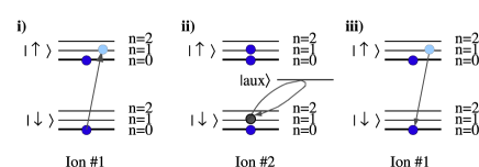
Figure 4: Cirac-Zoller Gate Scheme [7]. A phase gate is constructed by performing the sequence illustrated here: i) a $\pi$-pulse on the first blue sideband on the first ion to map the internal state to the collective vibrational state; ii) a $2\pi$-pulse between the $\left|\downarrow,n=1\right\rangle$ state and an auxiliary state $\left|aux\right\rangle$ on the second ion, resulting in a $\pi$ phase shift on the state $\left|\downarrow,n=1\right\rangle$; iii) a $\pi$-pulse on the first blue sideband on the first ion to map the vibrational state back to the internal state. A controlled-NOT gate can be constructed from a phase gate with a $\pi/2$-pulse on the second qubit before and after the phase gate. While the phase gate by definition maintains strict control of the qubit phase, the controlled-NOT gate relies on the two additional $\pi/2$-pulses having a particular phase with respect to the qubit.

Step (3) is identical to step (1) except the phase is shifted by $\pi.$ There are many ways to implement step (2), one of which is: i) a $\pi$-pulse blue sideband that maps the internal qubit state of the control qubit to the collective state of the ion pair, ii) a $2\pi$-pulse coupling the $\left|\downarrow_{2}\right\rangle\left|n=1\right\rangle$ state exclusively to an auxiliary level, and iii) a $\pi$-pulse on the blue sideband to map the collective motional state back to the control bit (see Figure 4). The net effect of these steps produces the following phase gate:

$$\begin{array}[]{rrr}\left|\uparrow\uparrow\right\rangle&\rightarrow&\left|\uparrow\uparrow\right\rangle\\ \left|\uparrow\downarrow\right\rangle&\rightarrow&\left|\uparrow\downarrow\right\rangle\\ \left|\downarrow\uparrow\right\rangle&\rightarrow&\left|\downarrow\uparrow\right\rangle\\ \left|\downarrow\downarrow\right\rangle&\rightarrow&-\left|\downarrow\downarrow\right\rangle\end{array}.$$ (10)

Here every state maintains a constant amplitude and the phase is well-defined. However, steps (1) and (3) contribute an additional phase to the controlled-NOT gate:

$$\begin{array}[]{rrr}\left|\uparrow\uparrow\right\rangle&\rightarrow&\left|\uparrow\uparrow\right\rangle\\ \left|\uparrow\downarrow\right\rangle&\rightarrow&\left|\uparrow\downarrow\right\rangle\\ \left|\downarrow\uparrow\right\rangle&\rightarrow&e^{i\phi}\left|\downarrow\downarrow\right\rangle\\ \left|\downarrow\downarrow\right\rangle&\rightarrow&e^{i\phi}\left|\downarrow\uparrow\right\rangle\end{array}.$$ (11)

The phase of the Cirac-Zoller controlled-NOT gate therefore depends solely on the phase of the $\pi/2$-pulse single qubit rotations. As mentioned in section 1.1, the sensitivity of single qubit rotations to optical phase can be removed using copropagating Raman beams requiring only a stable microwave source driving an optical modulator. This conversion between a phase gate and a controlled-NOT gate is extremely useful for many entangling gate schemes, since phase gates are more intuitive to construct and have an inherently well-defined phase.

The CZ model for trapped ion quantum logic gates has many drawbacks, including the need for individually addressing the ions with optical sources, and the requirement that the motion be prepared in a pure state of collective motion, usually through laser-cooling to the $\left|0_{\nu}\right\rangle$ state. In the remainder of this paper, we consider improved schemes for trapped ion quantum gates that do not have these requirements. In some cases, we will see that the sensitivity to the optical phase $e^{i\Delta kX_{0,i}-i\Delta\phi}$ can also be suppressed.

2 Spin-Dependent Forces in the Resolved-Sideband Limit

Unlike the Cirac-Zoller gate where the internal qubit state of one ion is directly transferred to particular eigenstates of motion, entangling gates using spin-dependent forces coherently displace the initial motional state in the position/momentum phase space, a process through which each spin state can acquire an independent geometric phase[11, 14, 10, 16, 12]. The nonlinearity in these phases can result in a final state that can no longer be separated into two independent qubit subspaces, thus entangling the internal states of the two ions. This produces a phase gate similar to the Cirac-Zoller scheme, which can then be converted to a controlled-NOT gate when combined with single qubit rotations.

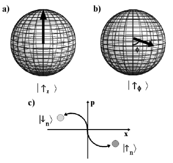
Figure 5: Representation of the eigenstate of a) $\mbox{\boldmath$\sigma$}\cdot\mathbf{z}$ and b) $\mbox{\boldmath$\sigma$}\cdot\mbox{\boldmath$\phi$}$ on the Bloch sphere corresponding to the eigenvalue $+1$. A spin-dependent force creates two separate coherent states in phase space corresponding to the eigenstates of $\mbox{\boldmath$\sigma$}\cdot\mathbf{n}$, as represented in c), thus entangling the internal spin with the external motion of the ion.

In this section, we focus on gates in the resolved-sideband limit where the interaction time is much longer than the trap period. The interaction Hamiltonian is proportional to $\hat{\mbox{\boldmath$\sigma$}}_{1}\cdot\mathbf{n}_{1}\otimes\hat{\mbox{\boldmath$\sigma$}}_{2}\cdot\mathbf{n}_{2}$, where $\hat{\mbox{\boldmath$\sigma$}}_{i}$ is the Pauli spin matrix operating on the internal qubit states, and $\mathbf{n}_{i}$ is a unit vector pointing in a particular direction on the Bloch sphere for ion $i$. The eigenstates of $\hat{\mbox{\boldmath$\sigma$}}_{1}\cdot\mathbf{n}_{1}\otimes\hat{\mbox{\boldmath$\sigma$}}_{2}\cdot\mathbf{n}_{2}$ each experiences a different force from the interaction (see Figure 5). The gates are categorized according to the direction of $\mathbf{n}_{i}$: in a “$\hat{\sigma}_{z}$ gate”, the differential force is applied via a differential AC Stark shift on the states $\left|\uparrow_{i}\right\rangle$ and $\left|\downarrow_{i}\right\rangle$ induced by the laser fields [16]. However, clock states exhibit no differential AC Stark shift when the Raman detuning $\Delta$ is large compared to the qubit frequency splitting $\omega_{0}$ (see Appendix A), so the only available qubit states for a $\hat{\sigma}_{z}$ gate are thus susceptible to magnetic field fluctuations. In a “$\hat{\sigma}_{\phi}$ gate”, optical fields driving spin flips and coupling to the motion produces a differential force between eigenstates of $\hat{\mbox{\boldmath$\sigma$}}_{i}\cdot\mbox{\boldmath$\phi$}_{i}$, where the unit vector $\mbox{\boldmath$\phi$}_{i}=\cos(\phi_{i})\mathbf{x}+\sin(\phi_{i})\mathbf{y}$ lies on the equatorial plane of the Bloch sphere[14, 10, 27, 17]. Although this gate is compatible with clock states, the optical beam configuration can give rise to extreme sensitivity of the qubit phase on the optical phase of the driving field, which can be the limiting factor in the fidelity of the gate[27]. In this section, we propose a method to cancel this phase dependence on the optical field, relaxing the constraint on long-term interferometric stability between the two Raman beam paths for the entirety of a multi-gate sequence quantum algorithm.

2.1 Forced Quantum Harmonic Oscillator

In order to understand the spin-dependent force, we start by considering the effects when a force is applied to a harmonic oscillator. In general, a forced harmonic oscillator has a Hamiltonian of the form [28]

$$\hat{H}=\hbar\omega(\hat{a}^{\dagger}\hat{a}+\frac{1}{2})+f^{*}(t)x_{0}\hat{a}+f(t)x_{0}\hat{a}^{\dagger},$$ (12)

where $\hat{a}$ and $\hat{a}^{\dagger}$ are the annihilation and creation operators respectively, and $x_{0}=\sqrt{\hbar/(2M\omega)}$ is the root mean square spatial spread of the ground state wavepacket. The first term is the unperturbed Hamiltonian for the harmonic oscillator of frequency $\omega$, and the last two terms correspond to an external time-dependent force $f(t)$ applied to the system. In the interaction picture

$$\hat{H}_{I}(t)=f^{*}(t)x_{0}\hat{a}e^{-i\omega t}+f(t)x_{0}\hat{a}^{\dagger}e^{i\omega t}.$$ (13)

Assuming the force $f(t)=Fe^{-i(\omega-\delta)t}/2$ is detuned from resonance by frequency $\delta\ll\omega$, then the interaction Hamiltonian can be rewritten as

$$\hat{H}_{I}(t)=\frac{F^{*}x_{0}}{2}\hat{a}e^{-i\delta t}+\frac{Fx_{0}}{2}\hat{a}^{\dagger}e^{i\delta t}.$$ (14)

The state after an interaction time $t$ is prescribed by the time-evolution operator

$$\hat{U}(t)=\exp\left\{-\frac{i}{\hbar}\left(\int_{0}^{t}\hat{H}_{I}(t^{\prime})dt^{\prime}+\frac{1}{2}\int_{0}^{t}dt^{\prime}\int_{0}^{t^{\prime}}dt^{\prime\prime}[\hat{H}_{I}(t^{\prime}),\hat{H}_{I}(t^{\prime\prime})]+...\right)\right\}.$$ (15)

If we consider only the first term in the exponent of the evolution operator and substituting in the interaction Hamiltonian from Equation 14, the resulting operator is exactly the displacement operator

$$\hat{D}(\alpha)=e^{\alpha\hat{a}^{\dagger}+\alpha^{*}\hat{a}},$$ (16)

with $\alpha$ defined as

$$\alpha(t)=-\frac{i}{\hbar}\int_{0}^{t}\frac{Fx_{0}}{2}e^{i\delta t^{\prime}}dt^{\prime}.$$ (17)

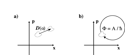
Figure 6: a) Displacement in phase space, in a frame rotating at the natural frequency of the harmonic oscillator. The displacement operator translates motional states in position/momentum phase space without distortion. b) For a force detuned from resonance, the motional state follows a circular path. For a closed trajectory, the quantum state acquires a geometric phase $\phi=A/\hbar$ in a round-trip orbit, where $A$ is the area enclosed by the trajectory.

The displacement operator translates motional states in position/momentum phase space without distortion (Figure 6). For example, a displacement on an initial ground state of motion results in a coherent state $\left|\alpha\right\rangle=\hat{D}(\alpha)\left|0\right\rangle$, where the final state is defined in terms of number states as $\left|\alpha\right\rangle=e^{-\frac{1}{2}\left|\alpha\right|^{2}}\sum_{n=0}^{\infty}\frac{\alpha^{n}}{\sqrt{n!}}\left|n\right\rangle.$ In terms of x-p coordinates, $\alpha=(1/2x_{0})(x+ip/M\omega)$.

The remaining higher order terms in the time-evolution operator originate from the non-commutative property of the interaction Hamiltonian at a given time with itself at different times. This can be understood by considering the displacement operators, which do not commute with one another but rather follow the commutation rule $\hat{D}(\alpha)\hat{D}(\beta)=\hat{D}(\alpha+\beta)e^{iIm(\alpha\beta^{*})}$. Therefore the complete time-evolution operator can be constructed by integrating over infinitesimal displacements in time:

$$\hat{U}(t)=e^{i\Phi(t)}\hat{D}(\alpha(t)),$$ (18)

with the geometric phase accumulated over the entire path from time $0$ to $t$ expressed as

$$\Phi(t)=Im(\int_{0}^{t}\alpha(t^{\prime})^{*}d\alpha(t^{\prime})).$$ (19)

For a near-resonant driving force with detuning $\delta$ (Equation 14), the initial motional state moves in a circular trajectory of radius $F/(2\hbar\delta)$ with periodicity $T=2\pi/\delta$ in the rotating frame of harmonic motion, following the path (from Equation 17)

$$\alpha(t)=\frac{Fx_{0}}{2\hbar\delta}\left(1-e^{i\delta t}\right).$$ (20)

In one period of evolution under this force, the motional state returns to its original phase space coordinates, but acquires a geometric phase of

$$\Phi_{0}=\frac{\pi\left|Fx_{0}\right|^{2}}{2(\hbar\delta)^{2}}$$ (21)

equivalent to the area enclosed by the trajectory (Figure 6).

For a single qubit experiencing a spin-dependent force, the interaction Hamiltonian includes a dependence on the internal spin state of the ion. Assuming the force couples to only one of the vibrational modes and the other mode can be neglected under the rotating wave approximation, the most general expression for the interaction Hamiltonian is

$$\hat{H}_{I}=\sum_{m=\uparrow_{\mathbf{n}},\downarrow_{\mathbf{n}}}\left(\frac{F_{m}^{*}x_{0}}{2}\hat{a}e^{-i\delta t}+\frac{F_{m}x_{0}}{2}\hat{a}^{\dagger}e^{i\delta t}\right)\left|m\right\rangle\left\langle m\right|,$$ (22)

where $m$ denotes the internal qubit state of the ion, and $\left|\uparrow_{\mathbf{n}}\right\rangle$ and $\left|\downarrow_{\mathbf{n}}\right\rangle$ are the eigenstates of $\hat{\mbox{\boldmath$\sigma$}}\cdot\mathbf{n}$ associated with eigenvalues $+1$ and $-1$ respectively. The interaction provides no coupling between the two orthogonal spin eigenstates of $\hat{\mbox{\boldmath$\sigma$}}\cdot\mathbf{n}$, but the motional state becomes entangled with the spin state as the differential force pushes the motional states of the two spin components in separate directions. At time $t=2n\pi/\delta$, where $n$ is an integer, the two motional states overlap again, disentangling the vibrational component of the wavefunction from the spin, but leaving the spin component with a phase shift due to the difference in the geometric phases of the paths. The interaction Hamiltonian can also be written in terms of the $\hat{\mbox{\boldmath$\sigma$}}\cdot\mathbf{n}$ operator as follows:

$$\hat{H}_{I}=\left(\frac{F_{+}^{*}x_{0}}{2}\hat{a}e^{-i\delta t}+\frac{F_{+}x_{0}}{2}\hat{a}^{\dagger}e^{i\delta t}\right)\hat{I}+\left(\frac{F_{-}^{*}x_{0}}{2}\hat{a}e^{-i\delta t}+\frac{F_{-}x_{0}}{2}\hat{a}^{\dagger}e^{i\delta t}\right)\hat{\mbox{\boldmath$\sigma$}}\cdot\mathbf{n},$$ (23)

where $\hat{I}$ is the identity operator, $F_{+}=(F_{\uparrow_{\mathbf{n}}}+F_{\uparrow_{\mathbf{n}}})/2$ and $F_{+}=(F_{\uparrow_{\mathbf{n}}}-F_{\uparrow_{\mathbf{n}}})/2$.

Now consider a spin-dependent force applied simultaneously to two ions in the same trapping potential. The total force on the system is now dependent on the spins of both ions. The interaction Hamiltonian now becomes

$$\hat{H}_{I}=\sum_{m1,m2=\uparrow_{\mathbf{n}},\downarrow_{\mathbf{n}}}\left(\frac{F_{m1,m2}(t)x_{0}}{2}\hat{a}^{\dagger}+\frac{F_{m1,m2}^{*}(t)x_{0}}{2}\hat{a}\right)\left|m1,m2\right\rangle\left\langle m1,m2\right|,$$ (24)

where $m_{1}$, $m_{2}$ denotes the internal qubit state of ion 1 and ion 2 respectively, and $F_{m1,m2}=F_{m1}+F_{m2}$ is the total force applied to the state $\left|m1,m2\right\rangle$. The geometric phase of an enclosed loop is proportional to $\left|F_{m_{1},m_{2}}x_{0}\right|^{2}/\delta$ (Equation 21), which can be calibrated so that the nonlinearity results in a wavefunction whose spins are not factorizable, thus creating entanglement between two ions.

The following sections will provide specific examples of entangling gates using spin-dependent forces. While the fundamental concept is the same in both instances, the experimental requirements and the susceptibility to various sources of phase decoherence are distinct. We will discuss these cases in detail and provide some solutions for phase control of these gates.

2.2 The $\hat{\sigma}_{z}$-gate

As the name implies, the $\hat{\sigma}_{z}$-gate applies a differential force on the eigenstates of the unperturbed Hamiltonian. The interaction has no coupling between the two eigenstates of $\hat{\sigma}_{z}$, conveniently avoiding the neccessity to produce large frequency shifts in the Raman beams to bridge the hyperfine splitting. Instead, the Raman beams couple to the vibrational states without driving a spin flip. The two Raman beams form a beating wave with periodicity $2\pi c/(\omega_{\nu}-\delta)$ along the weakest trap dimension. Due to the AC Stark effect, this wave form a moving periodic potential, exerting a near-resonant force on the ion in the direction of travel. If the AC Stark effect has different amplitude on the two qubit states, then the two states experience different forces from the beating wave [16].

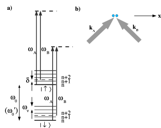
Figure 7: A $\sigma_{z}$-dependent force is driven by electromagnetic fields with two frequencies separated by $\omega_{\nu}+\delta$, as shown in a). These fields couple the two qubit states to the excited states with different coupling strengths (depending on polarization), producing a differential AC Stark shift that oscillates at $\omega_{\nu}+\delta$. The two fields must have a non-zero wave-vector difference $\Delta\mathbf{k}=\mathbf{k}_{B}-\mathbf{k}_{A}$ with a component in the $x$ direction.

The $\hat{\sigma}_{z}$ gate uses two non-copropagating beams with frequency difference $\omega_{\nu}-\delta$, where $\omega_{\nu}$ is the frequency of vibration and $\delta$ is the detuning from the vibration frequency. For this example, we will let the beams couple to the stretch mode $\omega=\omega_{2}=\sqrt{3}\omega_{1}$, though the same algebra can be carried out for the center-of-mass mode. (Stretch mode is a better candidate since it exhibits lower levels of decoherence from background electric fields [18].) We apply two fields $E_{A}e^{i(\mathbf{k}_{A}\cdot\mathbf{x}-\omega_{A}t-\phi_{A})}\mbox{\boldmath$\epsilon$}_{A}+E_{B}e^{i(\mathbf{k}_{B}\cdot\mathbf{x}-\omega_{B}t-\phi_{B})}\mbox{\boldmath$\epsilon$}_{B}$ where the frequency difference $\omega_{B}-\omega_{A}=\omega_{2}-\delta$ is slightly detuned from the stretch mode frequency. The field couples each of the spin states to the excited $P$ state, and is detuned by a large frequency $\Delta$ (see Figure 7). Using the same RWA and adiabatic elimination of the excited state used to obtain Equation 3, the interaction Hamiltonian for a single ion becomes

$$\hat{H}_{I}=\frac{\hbar}{4\Delta}\left\{\left[\left|g_{\uparrow A}\right|^{2}+\left|g_{\uparrow B}\right|^{2}+\left(2g_{\uparrow A}^{*}g_{\uparrow B}e^{i(\Delta\mathbf{k}\cdot\hat{\mathbf{R}}-(\omega_{2}-\delta)t-\Delta\phi)}+h.c.\right)\right]\left|\uparrow\right\rangle\left\langle\uparrow\right|\right.$$

$$+\left.\left[\left|g_{\downarrow A}\right|^{2}+\left|g_{\downarrow B}\right|^{2}+\left(2g_{\downarrow A}^{*}g_{\downarrow B}e^{i(\Delta\mathbf{k}\cdot\hat{\mathbf{R}}-(\omega_{2}-\delta)t-\Delta\phi)}+h.c.\right)\right]\left|\downarrow\right\rangle\left\langle\downarrow\right|\right\}$$ (25)

where $g_{m,l}=\mbox{\boldmath$\mu$}_{m}\cdot\mbox{\boldmath$\epsilon$}_{l}E_{l}/2\hbar$ is the single photon Rabi frequencies associated with each field $l$ coupling qubit state $\left|m\right\rangle$ to excited level $\left|e\right\rangle$, $\Delta\mathbf{k}=\mathbf{k}_{B}-\mathbf{k}_{A}$ is the wave vector difference, and $\Delta\phi=\phi_{B}-\phi_{A}$ is the phase difference between the driving fields. The first two terms in the expressions in Equation 25 contribute to the average Stark shift for each of the states, which can be canceled by carefully choosing the polarizations $\mbox{\boldmath$\epsilon$}_{1}$ and $\mbox{\boldmath$\epsilon$}_{2}$ [16]. The cross terms represent the variation in intensity formed by the interference pattern that pushes the ion, and must have a different magnitude and/or phase between the two qubit states to create a differential force. In the Lamb-Dicke limit, and assume the detuning $\Delta$ is approximately the same for both spin states ($\Delta\gg\omega_{0}$), the interaction Hamiltonian for two ions can be written as

$$\hat{H}_{I}=\frac{\hbar}{2}\sum_{i=1,2}\sum_{m_{i}=\uparrow,\downarrow}\eta_{2}\Omega_{m_{i}}D^{\prime}_{n_{2},n_{2}^{\prime}}\left(\hat{a}_{2}e^{-i(\delta t-\phi_{i})}+\hat{a}_{2}^{\dagger}e^{i(\delta t-\phi_{i})}\right)\left|m_{i}\right\rangle\left\langle m_{i}\right|$$

$$\hbox to0.0pt{\hss${}={}$}\sum_{m_{1},m_{2}=\uparrow,\downarrow}\left(\frac{F_{m_{1},m_{2}}^{*}q_{2}}{2}\hat{a}_{2}e^{-i\delta t}+\frac{F_{m_{1},m_{2}}q_{2}}{2}\hat{a}_{2}^{\dagger}e^{i\delta t}\right)\left|m_{1}m_{2}\right\rangle\left\langle m_{1}m_{2}\right|,$$ (26)

where $F_{m_{1},m_{2}}q_{2}=(\hbar\eta_{2}D^{\prime}_{n_{2,}n_{2}}/\Delta)(g_{m_{1},A}^{*}g_{m_{1},B}e^{i\phi_{1}}-g_{m_{2},A}^{*}g_{m_{2},B}e^{i\phi_{2}})$, and $\phi_{i}=\Delta kX_{0,i}-\Delta\phi$.

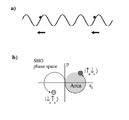
Figure 8: The spacing of the two ions determines the relative phase of the optical field experienced by each ion. a) The ions drawn are spaced by an integer multiple of the optical wavelength, creating an equal force on the two ions given the same internal state. In this scenario, b) spin states with opposite parity can excite the stretch mode, and the geometric phase acquired by each state is proportional to the area covered by the trajectory in phase space ($\pi/2$ for the phase gate shown in Equation 27). The spin states with the same parity remain at the origin (not shown here) and acquire no geometric phase.

The phase difference between the force applied to the two ions is determined by the optical phase difference $\phi_{1}-\phi_{2}$, which corresponds to the ion spacing at equilibrium. If the ions are spaced by an integer multiple of the optical wavelength, i.e. $\Delta k(X_{0,1}-X_{0,2})=2n\pi$, then they experience the same phase in the force, i.e. $\phi_{1}=\phi_{2}$ (see Figure 8). This is a convenient case since the forces cancel when the two spins are aligned in the same direction, and displacement occurs only when the spins are anti-aligned. A physical explanation of this scenario is that the stretch mode can be excited only when the two ions are pushed in different directions or with different magnitudes. The fastest gate time possible for this scheme is when the anti-aligned states acquire a $\pi/2$ phase shift in time $T=2\pi/\delta$, or in other words, a round-trip geometric phase $\Phi_{0}=\pi\left|F_{\uparrow,\downarrow}q_{2}\right|^{2}/2(\hbar\delta)^{2}=\pi/2$. Under these conditions, and assuming all the average Stark shifts have been accounted for, the gate performs the operation [16, 11]:

$$\begin{array}[]{rrr}\left|\uparrow\uparrow\right\rangle&\rightarrow&\left|\uparrow\uparrow\right\rangle\\ \left|\uparrow\downarrow\right\rangle&\rightarrow&i\left|\uparrow\downarrow\right\rangle\\ \left|\downarrow\uparrow\right\rangle&\rightarrow&i\left|\downarrow\uparrow\right\rangle\\ \left|\downarrow\downarrow\right\rangle&\rightarrow&\left|\downarrow\downarrow\right\rangle\end{array}.$$ (27)

With a phase shift of $-\pi/2$ on both qubits, the final state is equivalent to the result from a standard phase gate in Equation 10.

Note that the end result is completely independent of the optical phase of the drive field. The optical phase $\phi_{i}$ is absorbed in the term $F_{m_{1},m_{2}}$, translating to a phase shift in $\alpha$ that defines the coherent state. Since the acquired geometric phase depends only on the area enclosed by the trajectory, the phase of the resulting state has no correlation to the phase of $F_{m_{1},m_{2}}$. While the optical phase still needs to be coherent during a gate, variations in phase between gates are acceptable since they have no impact on the outcome.

Ideally, if the $\hat{\sigma}_{z}$ gate can be performed on magnetic field insensitive states, the gate would be extremely phase stable. Unfortunately, in the limit where the detuning from the excited state is large compared to the hyperfine splitting, magnetic field insensitive states have no differential Stark shift (see Appendix A). Therefore, this gate is susceptible to decoherence from magnetic field fluctuations if performed on magnetic field sensitive states, or if performed on magnetic field insensitive states in the limit where detuning from excited state is comparable to the hyperfine splitting, by spontaneous emission from the excited state.

2.3 $\hat{\sigma}_{\phi}$-gate

We call the gate scheme proposed by Mølmer and Sørensen [14, 10] a $\hat{\sigma}_{\phi}$ gate because the interaction is analogous to the $\hat{\sigma}_{z}$ gate operating in a rotated basis. Although the original treatment describes the interaction in a four-level ladder system, here we describe it in terms of spins and displaced motional states as in section 2.1. The Mølmer-Sørensen gate employs simultaneous addressing of both ions with bichromatic fields, one detuned from the red sideband of a vibrational mode by frequency $\delta$ and the other from the blue sideband by $-\delta$. The two sidebands have equal strength $\eta_{\nu}\Omega/2$ in the Lamb-Dicke Limit, and once again we assume the force couples only to the stretch mode. The interaction Hamiltonian is simply the sum of the red sideband plus the blue sideband (from Equations 7 and 8) with a detuning $\delta$:

$$\hat{H}_{I}=-\frac{\hbar}{2}\sum_{i=1,2}\eta_{2}\Omega_{i}D^{\prime}_{n_{2},n^{\prime}_{2}}(e^{i(\Delta k_{r}X_{0,i}-\Delta\phi_{r})}\hat{\sigma}_{+}^{(i)}\hat{a}_{2}e^{-i\delta t}+e^{i(\Delta k_{b}X_{0,i}-\Delta\phi_{b})}\hat{\sigma}_{+}^{(i)}\hat{a}_{2}^{\dagger}e^{i\delta t}+h.c.),$$ (28)

where $\eta_{2}\Omega_{0}D^{\prime}_{n_{2},n^{\prime}_{2}}$ is the sideband Rabi frequency, $\Delta k_{r}$ and $\Delta k_{b}$ are the wave-vector difference for the red and blue sidebands, $X_{0,i}$ indicates the equilibrium position of the $i$-th ion along the x-axis, and $\Delta\phi_{r}$ and $\Delta\phi_{b}$ are the phases of the red and blue sidebands respectively. We can simplify this expression to:

$$\hat{H}_{I}=\sum_{i=1,2}\frac{F_{i}q_{2}}{2}\hat{\sigma}_{\phi_{S,i}}(e^{i\phi_{M,i}}\hat{a}_{2}e^{i\delta t}+e^{-i\phi_{M,i}}\hat{a}_{2}^{\dagger}e^{-i\delta t})$$

$$\indent=\sum_{m_{1}=\uparrow_{\phi_{S,1}},\downarrow_{\phi_{S,1}}}\sum_{m_{2}=\uparrow_{\phi_{S,2}},\downarrow_{\phi_{S,2}}}\left(\frac{F_{m_{1},m_{2}}^{*}q_{2}}{2}\hat{a}_{2}e^{i\delta t}+\frac{F_{m_{1}m_{2}}q_{2}}{2}\hat{a}_{2}^{\dagger}e^{-i\delta t}\right)\left|m_{1}m_{2}\right\rangle\left\langle m_{1}m_{2}\right|,$$

(29)

where

$$\hat{\sigma}_{\phi_{S,i}}^{(i)}=\hat{\mbox{\boldmath$\sigma$}}_{i}\cdot\left[\cos(\phi_{S,i})\mathbf{x}+\sin(\phi_{S,i})\mathbf{y}\right]=\hat{\sigma}_{+}^{(i)}e^{-i\phi_{S,i}}+\hat{\sigma}_{-}^{(i)}e^{i\phi_{S,i}}.$$ (30)

Here $F_{i}=\hbar\eta_{2}\Omega_{i}D^{\prime}_{n_{2},n^{\prime}_{2}}/q_{2}$ is the differential force on the $i$-th ion, $\phi_{S,i}=-(\Delta k_{r}X_{0,i}-\Delta\phi_{r}+\Delta k_{b}X_{0,i}-\Delta\phi_{b})/2$ is the spin phase of the $i$-th ion, $\phi_{M,i}=(\Delta k_{r}X_{0,i}-\Delta\phi_{r}-\Delta k_{b}X_{0,i}+\Delta\phi_{b})/2$ is the phase of the force on the $i$-th ion, and $F_{m_{1},m_{2}}=\pm F_{1}e^{-i\phi_{M,1}}\pm F_{2}e^{-i\phi_{M,2}}$ where $\pm F_{i}$ corresponds to the force on the spin state $m_{i}=\uparrow_{\mathbf{\phi}_{S,i}},\downarrow_{\mathbf{\phi}_{S,i}}$ respectively on the $i$-th ion. As in the $\hat{\sigma}_{z}$ gate, we set the phase of the force acting on the two ions to be opposite, i.e. $F_{1}e^{i\phi_{M,1}}=-F_{2}e^{i\phi_{M,2}}$, and choose $\delta$ and $F$ such that the round-trip geometric phase satisfies the condition $\Phi_{0}=2\pi\left|F_{1}q_{2}\right|^{2}/(\hbar\delta)^{2}=\pi/2$. Then the final state of the gate is equivalent to the final state in Equation 27, except $\left|\uparrow_{i}\right\rangle$ and $\left|\downarrow_{i}\right\rangle$, the eigenstates of $\hat{\sigma}_{z}^{(i)}$, are replaced by $\left|\uparrow_{\mathbf{\phi}_{S,i}}\right\rangle$ and $\left|\downarrow_{\mathbf{\phi}_{S,i}}\right\rangle$, the eigenstates of $\hat{\sigma}_{\mathbf{\phi}_{S,i}}^{(i)}$. This gate written in the $\hat{\sigma}_{z}$ basis produces the following truth table:

$$\begin{array}[]{ccl}\left|\uparrow\uparrow\right\rangle&\rightarrow&\frac{1}{\sqrt{2}}\left\{\left|\uparrow\uparrow\right\rangle-ie^{i(\phi_{s1}+\phi_{s2})}\left|\downarrow\downarrow\right\rangle\right\}\\ \left|\uparrow\downarrow\right\rangle&\rightarrow&\frac{1}{\sqrt{2}}\left\{\left|\uparrow\downarrow\right\rangle-i\left|\downarrow\uparrow\right\rangle\right\}\\ \left|\downarrow\uparrow\right\rangle&\rightarrow&\frac{1}{\sqrt{2}}\left\{\left|\downarrow\uparrow\right\rangle-i\left|\uparrow\downarrow\right\rangle\right\}\\ \left|\downarrow\downarrow\right\rangle&\rightarrow&\frac{1}{\sqrt{2}}\left\{\left|\downarrow\downarrow\right\rangle-ie^{-i(\phi_{s1}+\phi_{s2})}\left|\uparrow\uparrow\right\rangle\right\}\end{array}$$ (31)

Note that after the gate, only the spin phase remains, while the motion phase has no effect on the final state. As in the $\hat{\sigma}_{z}$ gate, drifts in the motion phase between gates is acceptable. However, the spin phase must be maintained between gates, or alternatively, an equivalent entangling gate with the dependence on the spin phase removed can be formed using a combination of $\hat{\sigma}_{\phi}$ gate and other quantum operations.

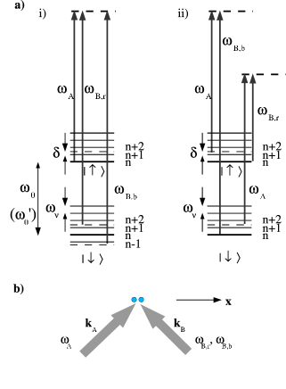
Figure 9: A $\hat{\sigma}_{\phi}$-dependent force is driven by electromagnetic fields with at least three optical frequencies as shown in a). Two frequencies separated by $\omega_{0}^{\prime}-\omega_{\nu}-\delta$ drive a detuned red sideband and a third frequency differs from one of them by $\omega_{0}^{\prime}+\omega_{\nu}+\delta$ to drive a detuned blue sideband. i) and ii) are two examples of possible frequency configurations. Some of the fields can have overlapping wave-vectors, but any pair of frequencies that drives a sideband must have a non-zero wave-vector difference with a component in the $x$ direction.

An analysis of noise sources for the spin phase requires careful consideration of the physical experimental setup in the laboratory. To drive the red sideband and the blue sideband transitions simultaneously, a minimum of three optical frequencies are required, assuming one frequency can be used for both sideband couplings (see Figure 9). Since each of the two fields driving a sideband must have a non-zero wave-vector difference $\Delta\mathbf{k}$, the optical beams can be set up such that two fields at different frequencies share the same wave-vector $\mathbf{k}_{B}$, and each individual field combined with a third field having a different wave-vector $\mathbf{k}_{A}$ drives a sideband transition. In other words, if the field along $\mathbf{k}_{A}$ has frequency $\omega_{A}$, then the field propagating along $\mathbf{k}_{B}$ needs both a frequency component $\omega_{A}\pm(\omega_{0}^{\prime}-\omega_{2}-\delta)$ to drive a detuned red sideband, and a frequency component $\omega_{A}\pm(\omega_{0}^{\prime}+\omega_{2}+\delta)$ to drive a detuned blue sideband. The choice of the positive or negative frequency differences between the fields determines the sign of $\Delta k_{r}$ and $\Delta k_{b}$, and determines the gate’s susceptibility to the phase stability between the two wave-vectors.

2.3.1 Phase sensitive geometry

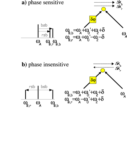
Figure 10: Possible beam configurations for the $\sigma_{\phi}$ gate. a) Phase sensitive configuration. The wave-vector difference for pairs of frequencies driving the red sideband and the blue sideband travel in the same direction $\Delta\mathbf{k}_{r}=\Delta\mathbf{k}_{b}$, using the frequency configuration shown in Figure 9 a) i) ). A phase shift $\delta\phi$ in one beam path results in a phase shift in the spin of the entangled state. b) Phase insensitive configuration. The wave-vector difference for pairs of frequencies driving the red sideband and the blue sideband travel in the opposite direction $\Delta\mathbf{k}_{r}=\Delta\mathbf{k}_{b}$, using the frequency configuration shown in Figure 9 a) ii). A phase shift $\delta\phi$ in one beam path results in no net phase shift in the spin of the entangled state.

The first scenario involves frequencies of both fields along $\mathbf{k}_{B}$ being higher (or lower) than $\omega_{A}$, then the wave-vector difference $\Delta\mathbf{k}$ for both the red and the blue sideband propagates in the same direction (Figure 10a). For example, let the field along $\mathbf{k}_{B}$ include both $\omega_{A}+\omega_{0}^{\prime}-\omega_{2}-\delta$ and $\omega_{A}+\omega_{0}^{\prime}+\omega_{2}+\delta$ frequency components. Then the wave-vector difference $\Delta\mathbf{k}_{r}=\mathbf{k}_{B}-\mathbf{k}_{A}=\Delta\mathbf{k}_{b}$ for the red sideband and the blue sideband point in the same direction. Instability in the relative beam paths results in an equal phase shift in the sideband transitions, i.e. $\delta\phi_{r}=\delta\phi_{b}=\delta\phi$. This results in a net shift in the spin phase by $\delta\phi_{S,i}=\delta\phi$. This is not a desirable situation since the outcome of the gate is sensitive to changes in the beam path length difference on the scale of an optical wavelength.

However, we note that the spin phase shift is exactly the same as the phase shift on the non-copropagating carrier transition, i.e. when the field propagating along $\mathbf{k}_{B}$ has frequency $\omega_{A}+\omega_{0}^{\prime}$. Therefore it is possible to construct a phase gate using the following Ramsey experiment: 1) Perform a $\pi/2$ rotation on both ion with phase shift $\delta\phi_{S,i}=\delta\phi$ using the non-copropagating transition; 2) Perform the $\hat{\sigma}_{\phi}$ gate using the frequencies listed above; 3) Perform a $-\pi/2$ rotation on both ions with phase shift $\delta\phi_{S,i}=\delta\phi$ using the non-copropagating transition. This rotation from $\mathbf{z}$ to $\mathbf{\phi}$ before the $\hat{\sigma}_{\phi}$ gate and the subsequent rotation back to $\mathbf{z}$ after the $\hat{\sigma_{\phi}}$ gate effectively removes the dependence on the spin phase $\phi$ as long as the spin phase is constant during the Ramsey experiment. The final state becomes identical to Equation 27 and has no residual dependence on $\delta\phi$. In addition, this scheme is also insensitive to ion spacing since the phase of the push force is always zero in the basis defined by $\phi_{S,i}$.

2.3.2 Phase insensitive geometry

Another scenario is to select the frequencies along $\mathbf{k}_{B}$ to straddle the frequency along $\mathbf{k}_{A}$. Then the wave-vector difference for the red and the blue sideband propagates in opposite directions. For example, let the field along $\mathbf{k}_{B}$ include both $\omega_{A}-(\omega_{0}^{\prime}-\omega_{2}-\delta)$ and $\omega_{A}+\omega_{0}^{\prime}+\omega_{2}+\delta$ frequency components (Figure 10b). Then the wave-vector difference for the red sideband $\Delta\mathbf{k}_{r}=-\mathbf{k}_{B}+\mathbf{k}_{A}=-\Delta\mathbf{k}_{b}$ is in the opposite direction as the blue sideband. Instability in the relative beam paths results in an opposite phase shift in the sidebands, i.e. $-\delta\phi_{r}=\delta\phi_{b}=\delta\phi$. This results in a net zero change in the spin phase $\delta\phi_{S,i}=0$, removing any spin phase dependence on $\delta\phi$ from the gate. Hence this configuration is termed “phase insensitive”.

However, the motion phase in this setup acquires a dependence on the phase shift $\delta\phi$. Therefore the phase of the force on each ion should be calibrated to be the same by setting the ion spacing (using the trap frequency as a tuning parameter) equal to $X_{0,1}-X_{0,2}=2n\pi/\Delta k$, where $n$ in an integer. While it is possible to produce similar entanglement operations with other values of ion spacing, the gate speed will be slower for the same intensity from the laser, and the output will appear different than the expression in Equation 31.

Similar to the other configuration, it is possible to construct a phase gate with the transformation in Equation 27, using an analogous Ramsey experiment involving single qubit rotations in phase with the gate: 1) Perform a $\pi/2$ rotation on both ion with phase shift $\delta\phi_{S,i}=0$ using either a calibrated and phase locked microwave source or a copropagating Raman transition; 2) Perform the $\sigma_{\phi}$ gate using the frequencies listed here; 3) Perform a $-\pi/2$ rotation on both ions with phase shift $\delta\phi_{S,i}=0$.

3 $\sigma_{z}$-gate with fast pulses

The $\sigma_{z}$-gate can also be achieved by applying spin-dependent momentum kicks on the ions with fast laser pulses [12, 29]. For gates in the resolved-sideband limit discussed in section 2, the ion is assumed to be confined within the Lamb-Dicke limit, where the spread in the position of the ions from their equilibrium positions is much smaller than the optical wave length. Outside of this limit, the effective Rabi frequency fluctuations leads to significant gate errors. For gates using fast laser pulses [12, 29], the impulsive spin-dependent force from the traveling wave has an almost uniform intensity distribution around the ion’s position, and this fluctuation of the effective Rabi frequency can be safely neglected. These pulsed gates can therefore faithfully operate outside of the Lamb-Dicke limit. In this section, we want to show that non-trivial phase errors can arise when the ions are outside the Lamb-Dicke limit, and suggest a method to cancel these errors by carefully selecting the direction and timing of momentum transfer, a technique reminiscent of the phase cancellation effect in the phase insensitive $\sigma_{\phi}$ gate configuration discussed in section 2.3.2.

The central component of the fast $\sigma_{z}$ gate in the context of ground state hyperfine qubits is a set of fast resonant laser pulse pairs that exclusively couple one of the two qubit states (here taken to be $\left|\downarrow\right\rangle$) of each ion to the excited state $\left|e\right\rangle$. The coupling Hamiltonian follows from from Equation 2 with $\Delta=0$:

$$\hat{H}_{I}=\hbar\sum_{i=1,2}-\left(\frac{g(t)}{2}e^{ik\cdot X_{0,i}-i\phi}e^{-i\eta_{1}(\hat{a}_{1}+\hat{a}_{1}^{\dagger})\mp i\eta_{2}(\hat{a}_{2}+\hat{a}_{2}^{\dagger})}\left|e_{i}\right\rangle\left\langle\downarrow\right|+h.c.\right)$$ (32)

where $g(t)$ is the resonant Rabi frequency of the transition for each ion and as before, the plus (minus) sign refers to ion $i=1$ ($i=2$). The pulse pairs are set to drive successive $\pi$-pulses ($\int_{0}^{\tau}g(t)dt=\pi$) from $\left|\downarrow_{i}\right\rangle\rightarrow\left|e_{i}\right\rangle\rightarrow\left|\downarrow_{i}\right\rangle$ on the electronic transitions of each ion, with the pulse duration $\tau$ taken to be much shorter than the radiative lifetime of $\left|e\right\rangle$ as well as the trap period $2\pi/\omega_{\nu}$.

When these two successive fast pulses have non-copropagating wave-vectors $\mathbf{k}_{A}$ and $\mathbf{k}_{B}$, and both $\pi$-pulses are completed in a time much shorter than the lifetime of state $\left|e_{i}\right\rangle$, the result is the following evolution for two ions [30, 12]:

$$\begin{array}[]{lll}\uparrow_{1}\uparrow_{2}\left|\alpha\right\rangle_{1}\left|\alpha\right\rangle_{2}&\rightarrow&\uparrow_{1}\uparrow_{2}\left|\alpha\right\rangle_{1}\left|\alpha\right\rangle_{2}\\ \uparrow_{1}\downarrow_{2}\left|\alpha\right\rangle_{1}\left|\alpha\right\rangle_{2}&\rightarrow&\uparrow_{1}\downarrow_{2}\left|\alpha+i\eta_{1}\right\rangle_{1}\left|\alpha-i\eta_{2}\right\rangle_{2}\\ \downarrow_{1}\uparrow_{2}\left|\alpha\right\rangle_{1}\left|\alpha\right\rangle_{2}&\rightarrow&\downarrow_{1}\uparrow_{2}\left|\alpha+i\eta_{1}\right\rangle_{1}\left|\alpha+i\eta_{2}\right\rangle_{2}\\ \downarrow_{1}\downarrow_{2}\left|\alpha\right\rangle_{1}\left|\alpha\right\rangle_{2}&\rightarrow&\downarrow_{1}\downarrow_{2}\left|\alpha+2i\eta_{1}\right\rangle_{1}\left|\alpha\right\rangle_{2}\end{array}.$$ (33)

In this expression, $\left|\alpha_{1}\right\rangle$ and $\left|\alpha_{2}\right\rangle$ are initial coherent states of the two modes of motion, and $\eta_{\nu}$ are the Lamb-Dicke parameters of the two modes associated with the wave-vector difference $\Delta\mathbf{k}_{j}\equiv\mathbf{k}_{A}-\mathbf{k}_{B}$, exactly as defined in section 1.1.

In the fast $\sigma_{z}$ gate, a series of pulse pairs is applied to the ions so that the motional states of both modes of motion simultaneously return to the same position in phase space regardless of the state of the two qubits. When these fast pulses are interspersed with periods of free evolution of the two modes of harmonic motion, the result can be a $\sigma_{z}$ phase gate for appropriate choices of pulse timing [12, 29]. This fast gate works independent of the motional state and outside of the Lamb-Dicke limit, as long as the motion remains harmonic.

However, outside of the Lamb-Dicke regime, we find that this gate can be sensitive to changes in the phase of the optical fields due to the change in the position of the ions at different times. In order to see this effect, we note that this fast $\sigma_{z}$-gate involves a spin-dependent force on the ion from absorption of a photon from a laser pulse traveling in the $\mathbf{k}_{A}$ direction and emission of another photon to a pulse propagating in a different $\mathbf{k}_{B}$ direction. We can lock the relative phase of these two propagating laser beams so that their phase difference is set to zero at the ion’s equilibrium position. Then, if during the above impulsive kicks, the ion is at a position $\mathbf{r}$ from its equilibrium site, it will acquire a net spin-dependent phase factor of $e^{i\Delta\mathbf{k}\cdot\mathbf{r}}$ from the absorption and the emission of the photon. This phase factor from each spin-dependent kick is non-negligible if the ion is outside of the Lamb-Dicke limit. For a complete gate operation with a series of laser kicks, with the spin-dependent phase factor for the $j$-th kick is denoted by $e^{i\Delta\mathbf{k}_{j}\cdot\mathbf{r}_{j}}$, the total phase factor after $N$ kicks is given by $e^{i\varphi_{t}}$ with $\varphi_{t}=\sum_{j=1}^{N}\left(\Delta\mathbf{k}_{j}\cdot\mathbf{r}_{j}\right)$. If the gate speed is comparable or slower than the local ion oscillation frequency, the ion’s position $\mathbf{r}_{j}$ at different laser kicks changes depending on the initial momentum and position are become almost uncorrelated. Therefore, the above effect contributes a random phase to the spin, which is a source of the gate infidelity.

To eliminate this random phase effect when the ion is outside the Lamb-Dicke limit, one needs to require the gate speed to be significantly faster than the local ion oscillation frequency. In that case, the ion’s position at different laser kicks are almost the same although they are still unknown. For any two positions $\mathbf{r}_{j}$ and $\mathbf{r}_{k}$ during the $j$-th and $k$-th kick respectively, the difference between them can be bounded as $\left|\mathbf{r}_{k}-\mathbf{r}_{j}\right|\lesssim vT_{g}$, where $v$ is the ion’s typical speed and $T_{g}$ denotes the gate time. Due to this position correlation and the fact that the total momentum kicks $\sum_{j=1}^{N}\Delta\mathbf{k}_{j}=0$ for the fast gate, we conclude that the random phase $\varphi_{t}$ is bounded by $\varphi_{t}\lesssim\left|\Delta\mathbf{k}_{j}\right|vT_{g}$, and the gate infidelity $\delta F\equiv 1-F$ from this random phase scales as $\left(\left|\Delta\mathbf{k}\right|vT_{g}\right)^{2}$. The scaling of $\delta F$ can be further improved to $\left(\left|\Delta\mathbf{k}\right|vT_{g}\right)^{2n}$ if we use a more involved sequence of the kicking forces with $n$ basic cycles. The gate time must be short enough to make the scaling parameter $\left|\Delta\mathbf{k}\right|vT_{g}<1$. Under that condition, the gate infidelity can then be reduced rapidly to zero with an appropriate pulse sequence even if the ion is outside of the Lamb-Dicke limit [29].

Conclusion

Most quantum logic gate schemes for trapped ions operate through interactions with optical electromagnetic fields. Some schemes, such as the $\sigma_{\phi}$ gate and the fast $\sigma_{z}$ gate, have a phase dependence on the phase of the optical driving field, which can become a major source of decoherence if uncontrolled. We have shown here methods to remove this phase dependence for these two entangling gates by choosing appropriate wave-vector orientations and pulse timings that naturally cancel the phase factor $e^{i\Delta\mathbf{k}\cdot\mathbf{r}}$ upon the completion of the gate. Furthermore, the sideband resolved $\sigma_{\phi}$ gate can operate on magnetic field insensitive qubit states, removing an unavoidable vulnerability of the $\sigma_{z}$ gate. These techniques eliminates the random phase from the optical driving field while maintaining phase coherence at the rf or microwave atomic frequencies, allowing long gate sequences to be performed over the timescales beyond the coherence time of the optical fields.

Appendix A Magnetic field insensitivity

In this appendix we will show that magnetic field insensitive states have no differential Stark shift in the limit where the detuning from the excited state is much larger than the hyperfine splitting, i.e. $\Delta_{HF}/\Delta\rightarrow 0$ [31]. To find the field insensitive states for a system in the $S_{1/2}$ ground state with some nuclear spin $I$, we write down the Hamiltonian for the hyperfine interaction in the presence of a magnetic field $\mathbf{B}$:

$$\hat{H}=\mbox{\boldmath$\mu$}_{B}\cdot\mathbf{B}+A\hat{\mathbf{I}}\cdot\hat{\mathbf{J}}=g_{J}\mathbf{B}\cdot\hat{\mathbf{J}}+g_{I}\mathbf{B}\cdot\hat{\mathbf{I}}+A\hat{\mathbf{I}}\cdot\hat{\mathbf{J}},$$ (34)

where $\hat{\mathbf{J}}$ is the total angular momentum of the electron, $\hat{\mathbf{I}}$ is the nuclear spin, and $A\hat{\mathbf{I}}\cdot\hat{\mathbf{J}}$ is the contact term. $g_{I}$ and $g_{J}$ are the Lande g-factors for the nucleus and the electron. The eigenstates of the Hamiltonian are linear combinations of the $m_{F}$ states, and can be represented as $\left|\Psi_{i}\right\rangle=a_{i}\left|g;m_{J}=\frac{1}{2},m_{I}=m_{F,i}-\frac{1}{2}\right\rangle+b_{i}\left|g;m_{J}=-\frac{1}{2},m_{I}=m_{F,i}+\frac{1}{2}\right\rangle$. The coefficients $a$ and $b$ are functions of the magnetic field. If two states $\left|\Psi_{1}\right\rangle$ and $\left|\Psi_{2}\right\rangle$ are magnetic field insensitive, then

$$\frac{\partial}{\partial B}\left(E_{1}-E_{2}\right)=0.$$ (35)

Applying Ehrenfest’s theorem,

$$\frac{\partial E_{i}}{\partial B}=\left\langle g_{J}J_{z}+g_{I}I_{z}\right\rangle=\left|a_{i}\right|^{2}\left[\frac{g_{J}}{2}+g_{I}(m_{F,i}-\frac{1}{2})\right]+\left|b_{i}\right|^{2}\left[\frac{g_{J}}{2}+g_{I}(m_{F,i}+\frac{1}{2})\right].$$ (36)

Normalization of the eigenstates and solving Equation 35 gives the result $\left|a_{1}\right|^{2}=\left|a_{2}\right|^{2}+g_{I}\Delta m_{F}/(g_{J}-g_{I})$. Since the dipole moment of the electron dominates the dipole moment of the nucleus, i.e. $g_{I}/g_{J}\approx 10^{-3}$, we can approximate it as

$$\left|a_{1}\right|^{2}=\left|a_{2}\right|^{2}$$

$$\left|b_{1}\right|^{2}=\left|b_{2}\right|^{2}.$$ (37)

Now consider the Stark shift for each of these magnetic field insensitive states. The AC Stark shift is given by

$$\chi_{i}=\sum_{m_{J},m_{I}}\frac{\left\langle\Psi_{i}\right|E\cdot d\left|e,m_{J}m_{I}\right\rangle\left\langle e,m_{J}m_{I}\right|E\cdot d\left|\Psi_{i}\right\rangle}{\Delta-E_{1}+E_{i}},$$ (38)

where $\left|e;m_{J},m_{I}\right\rangle$ is the excited state with the corresponding z-component of the electron and nuclear spins. Since the electric dipole only couples the orbital angular momentum of the electron, $\Psi_{i}$ only couples to the states with the same $m_{I}$. So the expression can be simplified to

$$\chi_{i}=\left|a_{i}\right|^{2}\sum_{m_{J}}\frac{\left|\left\langle g;m_{J}=\frac{1}{2}\right|E\cdot d\left|e,m_{J}\right\rangle\right|^{2}}{\Delta-E_{1}+E_{i}}+\left|b_{i}\right|^{2}\sum_{m_{J}}\frac{\left|\left\langle g;m_{J}=-\frac{1}{2}\right|E\cdot d\left|e,m_{J}\right\rangle\right|^{2}}{\Delta-E_{1}+E_{i}}.$$ (39)

If the energy difference between the two states $\Psi_{1}$ and $\Psi_{2}$ is small compared to $\Delta$, and applying the results from equation 37, then we find that $\chi_{1}=\chi_{2}$. So we conclude that the energy shift due to Stark effect is the same for any two magnetic field insensitive states.

Appendix B Driving stimulated Raman transitions using an Electro-optic Modulator

The fields driving stimulated Raman transition in ions are typically generated from a single laser source with the multiple frequencies generated by optical modulators. Acousto-optic modulators can produce frequency shifts up to about 1 GHz, while electro-optic modulators can modulate at upwards of 10 GHz or more. The electro-optic modulator offers a solution for driving Raman transitions in ion species with a large hyperfine splitting, but unlike acousto-optic modulators, all frequencies in the modulated field have the same wave-vector, making it difficult to separate different frequency components.

Electro-optic modulators control the birefringence of uniaxial crystals with a lower frequency electric field, effectively modulating either the phase or the polarization of the incident optical field, depending on the orientation of the optical axes. Since the Raman coupling is polarization-dependent, the polarization modulation is equivalent to an amplitude modulation. For non-copropagating Raman beam geometry, the modulated field is divided using a beam splitter and the two beams recombine at the trap from different angles. If the difference between any frequency from one beam and any frequency from the other beam matches the energy splitting of two atomic and/or phonon levels, then a transition can potentially be driven. However, the amplitude of each pair of frequencies driving the transition can result in cancellations in the total transition rate. Usually, amplitude modulation produces sidebands with the same phase, resulting in the transition rates adding constructively. But phase modulation produces a comb of sidebands, some having amplitudes with opposite phases, which could result in a total transition rate of zero. This problem can be remedied by setting the beam path length difference between the two beams to certain values that produces a non-zero total transition rate [32]. This effectively adds a different phase to each sideband, resulting in a transition rate proportional to the squared electric field

$$\Gamma_{k}(\phi)\sim\sum_{n=-\infty}^{\infty}J_{n}(\phi)e^{in\theta}J_{n+k}(\phi)e^{i(n+k)\theta}=J_{k}\left(2\phi\sin\left(\theta\right)\right)$$ (40)

where $J_{n}(x)$ is the $n$-th order Bessel function. Equation 40 describes the Raman transition rate involving the optical carrier and the $k$-th frequency modulated sideband with modulation index $\phi$ with a phase shift of $\theta=(\delta k\Delta x)mod(2\pi)$. Here $\delta k$ is the wave-number associated with the modulation frequency and $\Delta x$ is the beam path length difference.

To avoid nulling the average intensity due to destructive interference between the two fields at the ion, the field propagating along one path can be frequency shifted slightly from the field in the other path. The modulation frequency would then have to be adjusted to compensate for this frequency shift so that pairs of frequencies matches the energy difference between the two coupled levels. When the frequency offset is accounted for, all the $\Delta\mathbf{k}$ vectors driving the transition have the same sign, and the resulting transition is exactly the same as if each of the two beams having only a single frequency. To reverse the $\Delta\mathbf{k}$ vector, only the frequency offset on one beam needs to be changed. For example, to drive a Raman transition between two levels which have an energy splitting of $\hbar\omega_{transition}$, the modulation frequency of the EOM can be set to $\omega_{EO}<\omega_{transition}$. The modulated beam is split into two paths, with the beam in path A frequency shifted by $\omega_{offset}$ and the beam in path B frequency shifted by $\omega_{offset}+\omega_{transition}-\omega_{EO}$. The two beams are recombined at the ion, with wave-vector $\mathbf{k}_{A}$ and $\mathbf{k}_{B}$ respective to beam path A and B. In this case the wave-vector difference $\Delta\mathbf{k}$ for the Raman transition is equal to $\mathbf{k}_{B}$$-\mathbf{k}_{A}$, since the beam in path B has higher frequency. The beam in path B can also be frequency shifted by $\omega_{offset}+\omega_{EO}-\omega_{transition}$ instead, in which case the wave-vector difference $\Delta\mathbf{k}$ would be $\mathbf{k}_{A}-\mathbf{k}_{B}$ since the beam in path A would have the higher frequency.

The reversal of $\Delta\mathbf{k}$ is useful in the phase stable configuration for a $\sigma_{\phi}$ gate (see section 2.3.2). To generate red and blue sidebands with opposite wave-vector difference $\Delta\mathbf{k}_{r}=-\Delta\mathbf{k}_{b}$ , the frequency of the field along $\mathbf{k}_{B}$ can be shifted by $\omega_{offset}+\omega_{0}^{\prime}-\omega_{2}-\delta-\omega_{EO}$ to generate the red sideband and by $\omega_{offset}-\omega_{0}^{\prime}-\omega_{2}-\delta+\omega_{EO}$ to generate the blue sideband. These two frequencies can be arbitrarily close to one another by tuning the modulation frequency of the EO close to the qubit frequency splitting $\omega_{0}^{\prime}$, which allows both frequencies to be generated using a single frequency shifter with a given bandwidth. However, if the modulation frequency of the EO is exactly $\omega_{0}$, then each beam would simultaneously drive a copropagating carrier transition (see section 1.2.1) that will interfere with the $\sigma_{\phi}$ operation. Therefore the modulation frequency should be tuned to approximately but not exactly $\omega_{0}^{\prime}$.

References

Figure 2: Qubit with coherent Raman coupling via an excited state. Fields at frequency $\omega_{\alpha}$ and $\omega_{\beta}$ couple the qubit levels $\left|\uparrow\right\rangle$ and $\left|\downarrow\right\rangle$ via the excited state $\left|e\right\rangle$. The fields are detuned from the excited state resonances $\tilde{\omega}_{\uparrow,e}$ and $\tilde{\omega}_{\downarrow,e}$ by frequency $\Delta$.

Figure 3: Stimulated Raman transition between vibrational levels. Coupling depends on the beat note of the two Raman fields $\omega_{\beta}-\omega_{\alpha}$: a) $\omega_{0}^{\prime}$ for carrier transition, b) $\omega_{0}^{\prime}-\omega_{\nu}$ for first red sideband transition, and c) $\omega_{0}^{\prime}+\omega_{\nu}$ for first blue sideband transition. The qubit frequency splitting shifts from $\omega_{0}$ to $\omega_{0}^{\prime}$ due to AC Stark effect when the fields are turned on.

Figure 11: Demonstration of the phase sensitivity of the Mølmer-Sørensen ($\sigma_{\phi}$) force applied to a single ion using different beam configurations. (a) Pulse sequence of a photon-echo experiment for testing optical phase sensitivity of the $\sigma_{\phi}$ force. The echo pulses are carrier transitions driven by non-copropagating Raman beams propagating along the same wave-vectors as the $\sigma_{\phi}$ force, and an applied phase shift $\phi_{0}$ is added using an acousto-optic modulator that controls the timing of the pulse. The $\sigma_{\phi}$ force is applied for sufficient time such that the two motional states corresponding to spin states $\left|\uparrow_{\phi}\right\rangle$ and $\left|\downarrow_{\phi}\right\rangle$ have very little overlap at time $\tau$. A separate pulse in the other arm of the echo experiment cancels the residual AC Stark shift induced by the field driving the $\sigma_{\phi}$ force (the ratio $\omega_{0}/\Delta$ is significant enough to produce a non-negligible differential Stark shift between the two qubit states in this experiment) . (b) Probability of detecting $\left|\downarrow\right\rangle$ vs. applied shift in the phase of the echo pulses $\phi_{0}$ using the phase sensitive configuration described in section 2.3.1 and Figure 10a. The fringe contrast shows coherence between the phase $\phi$ in the $\sigma_{\phi}$ force and the phase $\phi_{0}$ in the Raman carrier pulses (Probability should vary sinusoidally from 0 to 0.5 when there is no decoherence). (c) Same plot using the phase insensitive configuration described in section 2.3.2 and Figure 10b. This time there is no coherence between the phase-insensitive $\sigma_{\phi}$ force and the phase-sensitive non-copropagating Raman carrier pulses.

Figure 12: Raman spectrum of two ions in the trap using a frequency comb generated by an electro-optic modulator (modulation frequency $\omega_{EO}-\omega_{0}=1.5$MHz in this case). The x-axis shows the frequency difference between the fields along the two beam paths. The carrier transition appears at $\pm 1.5$MHz ($C$), with corresponding first center-of-mass blue sideband transition at $\mp 0.6$MHz ($B_{1}$) $(\omega_{1}/2\pi=2.1$MHz) , first center-of-mass red sideband transition at $\pm 3.6$MHz ($R_{1}$), first stretch mode blue sideband at $\mp 2.1$MHz ($B_{2}$) $(\omega_{2}/2\pi=3.6$MHz), and first stretch mode red sideband at $\pm 5.1$MHz ($R_{2}$).

References

- [1] Divincenzo D P 2000 Fortschr. Phys., 48 771
- [2] Shor P W 1994 Proc. of the 35th Annual Symp. on the Foundations of Computer Science (New York: IEEE Computer Society Press) p 124
- [3] Grover L K 1997 Phys. Rev. Lett., 79 325
- [4] Shor P W 1995 Phys. Rev. A, 52 R2493
- [5] Steane A 1996 Phys. Rev. Lett., 77 793
- [6] Zurek W H 1999 Physics Today, 52 24
- [7] Cirac J I and Zoller P 1995 Phys. Rev. Lett., 74 4091
- [8] Wineland D J et al1998 J. Res. Nat. Inst. Stand. Tech. 103 259
- [9] Kielpinski D et al2002 Nature 417 709
- [10] Sørensen A and Mølmer K 1999 Phys. Rev. Lett. 82 1971
- [11] Milburn G J et al2000 Fortschr. Phys. 48 9, 801
- [12] Garcia-Ripoll J J et al2003 Phys. Rev. Lett. 91 157901
- [13] Häffner H et al2003 Phys. Rev. Lett. 90 143602
- [14] Mølmer K and Sørensen A 1999 Phys. Rev. Lett. 82 1835
- [15] Solano E et al1999 Phys. Rev. A 59 R2539
- [16] Leibfried D et al2003 Nature, 422 412
- [17] Haljan P C et al2005 Phys. Rev. Lett. 94 153602
- [18] Turchette Q A et al2000 Phys. Rev. A 61 063418
- [19] Deslauriers L et al2004 Phys. Rev. A 70 043408
- [20] Bollinger J J et al1991 IEEE Trans. Instr. Meas. 40 126
- [21] Paul W 1990 Rev. Mod. Phys. 62 531
- [22] Dehmelt H G 1967 Advances in Atomic and Molecular Physics, vol 3. (New York: Academic Press) p 53
- [23] Monroe C et al1995 Phys. Rev. Lett. 75 4714
- [24] Thomas J E et al1982 Phys. Rev. Lett. 48 867
- [25] Jaynes E T and Cummings F W 1963 Proc. of the IEEE 51 89
- [26] Schmidt-Kaler F et al2003 Nature 422 408
- [27] Sackett C A et al2000 Nature 404 256
- [28] Merzbacher E 1998 Quantum Mechanics (New York: John Wiley and Sons) p 335
- [29] Duan L M 2004 Phys. Rev. Lett. 93 100502
- [30] Poyatos J F et al1996 Phys. Rev. A 54 1532
- [31] Langer C et al2005 Preprint quant-ph/0504076
- [32] Lee P J et al2003 Optics Lett. 28 1852