Probabilistic programmable quantum processors with multiple copies of program state

Abstract

We examine the execution of general U(1) transformations on programmable quantum processors. We show that, with only the minimal assumption of availability of copies of the one-qubit program state, that the apparent advantage of existing schemes proposed by G.Vidal et al. [Phys. Rev. Lett. 88, 047905 (2002)] and M.Hillery et al. [Phys. Rev. A. 65, 022301 (2003)] to execute a general U(1) transformation with greater probability using complex program states appears not to hold.

I Introduction

In conventional classical computation, the data is manipulated by the computer (the “processor”) according the dictates of a program. Picking the program correctly ensures that the output data of the operation is as desired; the processor itself has general utility and can execute many different programs.

Nielsen and Chuang Nielsen97 have investigated the possibility of a general quantum processor. Modelling the processor as a quantum gate array into which we input a data state $|\psi\rangle_{d}$ represented by an array of qubits, and a program state $|\Xi\rangle_{p}$ that is also represented by an array of qubits, we can consider the operation of the quantum processor as effected by a unitary $G$:

$$|\psi\rangle_{d}\otimes|\Xi\rangle_{p}\rightarrow G[|\psi\rangle_{d}\otimes|\Xi\rangle_{p}].$$ (1)

In the case that the processor is to execute a particular unitary, $U$, on the data register, we would have:

$$G[|\psi\rangle_{d}\otimes|\Xi_{U}\rangle_{p}]=(U|d\rangle_{d})\otimes|\Xi_{U}^{{}^{\prime}}\rangle_{p},$$ (2)

as shown in Fig. 1, where $|\Xi_{U}\rangle_{p}$ is a program state to cause the execution of $U$ on the data state and it can be shown that the subsequent state of the program register, $|\Xi_{U}^{\prime}\rangle_{p}$, cannot be dependent on the data state, which for general processing will be unknown to us.

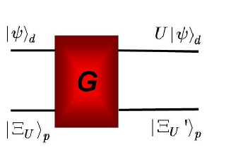
Figure 1: Model of a general quantum processor.

Nielsen and Chuang Nielsen97 have shown that a deterministic universal quantum processor of finite size does not exist. The problem is that a new dimension must be added to the program space for each unitary operator $U$ that one wants to be able to perform on the data $|\psi\rangle_{d}$. A similar situation holds if one studies quantum circuits that implement completely-positive, trace-preserving maps rather than just unitary operators Hillery2001 ; Hillery2002a . Some families of maps can be implemented with a finite program space, for example, the phase damping channel, but others, such as the amplitude damping channel, require an infinite program space. If one drops the requirement that the processor be deterministic, then universal processors become possible Nielsen97 ; Preskill1998 ; Vidal02 ; Hillery2002b . These processors are probabilistic: they sometimes fail, but we know when this happens.

In a probabilistic processor we demand that by measurement of the program register, we can tell whether the desired unitary operation has been performed on the data state or whether some other unitary operation has been performed upon it, i.e., that the state of the program register associated with the execution of $U$, $|\Xi_{U}^{\prime}\rangle_{p}$, is orthogonal to the states of the program register associated with other, undesired, outcomes on the data state (the identity of these states of the program register will in general be dependent on the nature of the processor itself). A model of this is shown in Fig. 2 where the outcome of the measurement of the program register, $|k\rangle_{p}$, indicates which unitary operation, $U_{k}$, has been performed on the data state.

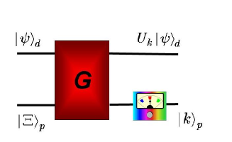
Figure 2: Model of a probabilistic general quantum processor. On the output of the program register a measurement is performed.

The simplest case of desired programmable operation on a qubit is the execution of a $U(1)$ transformation, $U(\theta)=e^{i\theta\sigma_{z}/2}$, upon a data qubit $|\psi\rangle_{d}=\alpha|0\rangle_{d}+\beta|1\rangle_{d}$. Here the unknown phase of the rotation $\theta$ is encoded in the programme state

$$|\Xi_{\theta}\rangle_{p}=\frac{1}{\sqrt{2}}\left(|0\rangle_{p}+e^{-i\theta}|1\rangle_{p}\right)\,,$$ (3)

while the processor itself is represented by a CNOT gate with data qubit as control and program qubit as target, followed by a measurement of the program qubit in the basis $\{|0\rangle_{p},|1\rangle_{p}\}$ (see Fig. 3).

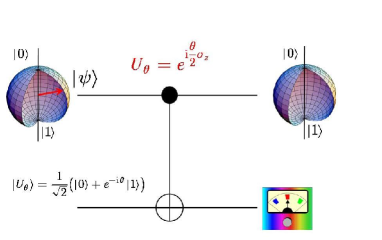
Figure 3: Model of a probabilistic CNOT quantum processor performing the $U(1)$ rotation of the input data state $|\psi\rangle$ by the angle $\theta$ that is encoded in the program state $|\Xi_{\theta}$ given by Eq. (3). On the output of the program register a measurement is performed.

The action of the CNOT processor on the data and the program input states is

$$|\psi\rangle_{d}|\Xi_{\theta}\rangle_{p} \longrightarrow \frac{1}{\sqrt{2}}U(\theta)|\psi\rangle_{d}|0\rangle_{p}$$ (4)

$$+\frac{1}{\sqrt{2}}U(-\theta)|\psi\rangle_{d}|1\rangle_{p}\,.$$

From this equation we see that when a projective measurement in the computer basis $\{|0\rangle,|1\rangle\}$ on the program qubit at the output of the CNOT is performed and the result $|0\rangle$ is registered then the data qubit that has been prepared in an unknown state $|\psi\rangle$ is rotated by the unknown angle $\theta$ as desired, i.e. with probability 1/2 we obtain the state $U(\theta)|\psi\rangle_{d}$ (see Fig. 4).

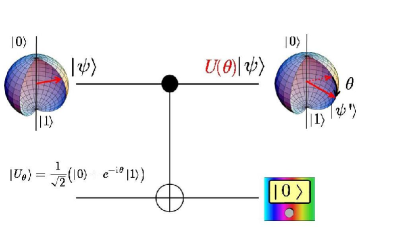
Figure 4: Model of a probabilistic CNOT quantum processor performing the $U(1)$ rotation of the input data state $|\psi\rangle$ by the angle $\theta$ that is encoded in the program state $|\Xi_{\theta}$. When the measurement performed on the program qubit result in the state $|0\rangle_{p}$ the desired rotation $U(\theta)$ is performed on the data qubit. The probability of success is equal to 1/2.

On the other hand, when the program qubit is measured in the state $|1\rangle_{p}$ then the data qubit is rotated in the opposite (“wrong”) direction, i.e. with probability 1/2 we obtain at the output of the probabilistic processor the state $U(-\theta)|\psi\rangle_{d}$ (see Fig. 5).

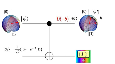
Figure 5: Model of a probabilistic CNOT quantum processor performing the $U(1)$ rotation of the input data state $|\psi\rangle$ by the angle $\theta$ that is encoded in the program state $|\Xi_{\theta}$. When the measurement performed on the program qubit results in the state $|1\rangle_{p}$ the rotation $U(-\theta)$ in the wrong direction is performed on the data qubit. The probability of this result is equal to 1/2.

In Sec. II we shall be considering three methods of increasing the success probability of this operation: the Vidal-Masanes-Cirac (VMC) Vidal02 method that uses a special $N$-qubit program state iteratively and terminates when a “good” result is achieved, the Hillery-Ziman-Bužek (HZB) Hillery03 scheme that uses the same program state as the VMC scheme but performs the operation in one step, and lastly in Sec. III we consider simply using $N$ copies of the basic program state $|\Xi_{\theta}\rangle$ given by Eq. (3). In the latter case, we consider three scenarios: iterative use of the program states, one-step use of the program states and, finally, preprocessing of the program states to produce a program state of the sort used by the VMC and HZB schemes, which is then put through a VMC or HZB processor. Sec. IV is devoted to conclusions and some technical details of our calculations are presented in Appendix.

II Increasing the probability of success

II.1 The VMC scheme

The probability of successfully carrying out the $U(1)$ operation on the data qubit can be increased through the enlargement of the program space Vidal02 ; Hillery03 . In the VMC scheme, if the first operation failed, that is, we performed $U(-\theta)$ on the data state, we could attempt to correct this by performing the rotation $U(2\theta)$ on the wrongly transformed data state $U(-\theta)|\Psi\rangle_{d}$ and if that failed we could attempt to perform the transformation $U(4\theta)$ on the data state $U(-3\theta)|\Psi\rangle_{d}$, etc. The $N$-qubit program state $|\Xi_{\theta}^{(N)}\rangle_{\vec{p}}$ used for this iterative operation can be written as

$$|\Xi_{\theta}^{(N)}\rangle_{\vec{p}} = |\Xi_{2^{N}\theta}\rangle_{p_{1}}\otimes|\Xi_{2^{N-1}\theta}\rangle_{p_{2}}\otimes\ldots\otimes|\Xi_{\theta}\rangle_{p_{N}}$$ (5)

$$= \frac{1}{\sqrt{2^{N}}}\sum_{j=0}^{2^{N}-1}e^{-ij\theta}|j\rangle_{\vec{p}},$$

with $|j\rangle_{\vec{p}}=|j_{N}\rangle_{p_{N}}\otimes|j_{N-1}\rangle_{p_{N-1}}\dots\otimes|j_{1}\rangle_{p_{1}}$, where $j_{l}$ is the $l$th bit in the binary representation of $j$.

II.2 The HZB scheme

Instead of using iteratively the CNOT processor following Ref. Hillery03 one can design a general quantum processor

$$G_{dp}=\sum_{j,k=1}^{2^{N}-1}A_{jk}\otimes|j\rangle_{p}\ \ {{}_{p}\langle k|}\,,$$ (6)

where $\{j\rangle_{p}|\ j=0,\ldots 2^{N}-1\}$ is an orthonormal basis for the program space and the $A_{jk}$ are operators acting on the data space such that:

$$\sum_{j=0}^{2^{N}-1}A_{xj}^{{\dagger}}A_{jy}=\sum_{j=0}^{2^{N}-1}A_{xj}A_{jy}^{{\dagger}}=I_{d}\delta_{xy}.$$ (7)

The result of the circuit on the combined data and program states input $|\Psi\rangle_{d}\otimes|\Xi\rangle_{p}\in{\cal H}_{d}\otimes{\cal H}_{p}$ can be expressed as:

$$G(|\Psi\rangle_{d}\otimes|\Xi\rangle_{p})=\sum_{j=0}^{2^{N}-1}A_{j}(\Xi)|\Psi\rangle_{d}\otimes|j\rangle_{p},$$ (8)

where the program operators $A_{j}(\Xi)$ are given by:

$$A_{j}(\Xi)=\sum_{k=0}^{2^{N}-1}{{}_{p}\langle k}|\Xi\rangle_{p}A_{jk}\,.$$ (9)

If the measurement of the program state returns $|n\rangle_{p}$, then Eq. (8) tells us that the operation $A_{n}(\Xi)$ has been carried out on the the data state.

To perform the $U(1)$ operation with only one iteration of the processor in the HZB scheme, we use the same program program state as for the VMC scheme given by Eq. (5). The circuit (processor) is then determined by the operators

$$A_{jk}=\delta_{j,k}|0\rangle_{d}{{}_{d}\langle 0|}+\delta_{j\oplus 1,k}|1\rangle_{d}{{}_{d}\langle 1|}$$ (10)

with $\oplus$ indicating addition modulo $2^{N}$. The program state is then measured and any result other than $|2^{N}-1\rangle_{p}$ indicates success. The success probability for this circuit is the same as that for the VMC circuit and it reads:

$$p=1-\frac{1}{2^{N}}\,.$$ (11)

This is the highest possible success probability achievable from the starting state $|\Xi_{\theta}^{(N)}\rangle_{p}$ for a general probabilistic quantum processor Vidal02 .

III Using multiple copies of the basic program state

III.1 Iterative process with multiple copies of the program state $|\Xi_{\theta}\rangle$

Given that $\theta$ is not known, it is not clear how the program states for the improved schemes above might in general be produced deterministically given no prior knowledge of $\theta$. General execution of $U(1)$ on a data qubit using a single program qubit and a CNOT gate is known to be optimally achieved using the program state $|\Xi_{\theta}\rangle$ given by Eq. (3) (see Ref. Ziman03 ), so assuming the availability of this state seems a reasonable minimal assumption. To increase the probability of success above 1/2 using just a CNOT, we require more copies of this basic program state and, if the operation $U(-\theta)$ has been carried out, we can reprocess the data state with a new copy of $|\Xi_{\theta}\rangle$ and continue this process until the desired transformation has been executed or until the available program states are exhausted . If $N$, the number of available copies of $|\Xi_{\theta}\rangle$, is an odd number (there is no benefit to using an even number of program states), the probability $p$ of succeeding before running out of copies of $|\Xi_{\theta}\rangle$ is given by the expression

$$p=1-\frac{1}{2^{N}}\left(\begin{array}[]{c}N\\ (N-1)/2\end{array}\right),$$ (12)

and, in the limit of large $N$:

$$p_{N\rightarrow\infty}=1-\sqrt{\frac{2}{\pi N}}.$$ (13)

III.2 Single-shot process with multiple copies of the program state $|\Xi_{\theta}\rangle$

The process can be carried out with one iteration of a larger gate array where we use an odd number of program qubits $N$ so that our combined program and data state is:

$$|\psi\rangle_{d}\otimes|\Xi_{\theta}\rangle_{p}^{\otimes N}=\frac{|\psi\rangle_{d}}{\sqrt{2^{N}}}\otimes\sum_{j=0}^{2^{N}-1}e^{-i|j|\theta}|j\rangle_{\vec{p}},$$ (14)

where $|j|$ is the Hamming weight of the binary representation of $j$ and we use the same basis for the program space as previously. Putting $A_{kk}=|0\rangle_{d}{{}_{d}}\langle 0|$ as before, we select the position of the terms $A_{jk}=|1\rangle_{d}{{}_{d}}\langle 1|$ according to the Hamming weight of the $j$ and $k$ such that

$$|k|=|j|+1$$ (15)

to the largest extent possible so that Eq. (7) is obeyed and we can position the other terms arbitrarily so as to respect Eq. (7). Where we can give the $A_{jk}$ values according to Eq. (15), measurement in the program basis will, up to global phase, ensure that the data qubit has been transformed by $U(\theta)$. The rows (values of $j$) where $A_{jk}=|1\rangle_{d}{{}_{d}}\langle 1|$ are not positioned according to $|k|=|j|+1$ indicate measurement outcomes where the desired transformation has not been carried out but instead a rotation through some negative multiple of $\theta$ has occurred. The number $R$ of rows that cannot be created so that Eq. (15) is obeyed is given by:

$$R=\left(\begin{array}[]{c}N\\ (N-1)/2\end{array}\right)$$ (16)

Each (incorrect) program operator corresponding to one of these rows has probability $2^{-N}$ so again the success probability is given by Eq. (12).

III.3 Preprocessing

If we wish to use, from a starting state of multiple copies of $|\Xi_{\theta}\rangle$, the VMC or HZB schemes, we can process these copies to produce a state of the form given in Eq. (5) that can then be used as the program state for the VMC or HZB processors. The $X-$qubit program state $|\Xi_{\theta}^{(X)}\rangle_{p}$ can be probabilistically constructed from a minimum of $N=2^{X}-1$ copies of $|\Xi_{\theta}\rangle$, and so it is possible, by preprocessing these copies of $|\Xi_{\theta}\rangle$, to construct, with some probability, a state $|\Xi(\theta)_{s}\rangle_{p}$ where $s\leq X$. A preprocessing scheme that produces the same overall probability of success, in executing $U(\theta)$ on a data qubit, as the schemes in Sec. II can be constructed by permuting the phases in $|\Xi_{\theta}\rangle^{\otimes 2^{X}-1}$ and making a measurement in the computational basis, initially on $2^{X}-1-X=M$ of the qubits.

We give two specific examples, of preprocessing. Firstly, we will assume to have three identical program states $|\Xi_{\theta}\rangle^{\otimes 3}$. Then we will consider the case with seven identical program states, i.e. $|\Xi_{\theta}\rangle^{\otimes 7}$. Using 3 and 7 program state we can probabilistically prepare the program states $|\Xi_{\theta}^{(2)}\rangle_{p}$ and $|\Xi_{\theta}^{(3)}\rangle_{p}$, respectively. In the Appendix we will quote the result for general $N$.

III.3.1 Preprocessing with three copies of $|\Xi_{\theta}\rangle$

We have that:

$$|\Xi_{\theta}\rangle^{\otimes 3} = \frac{1}{2\sqrt{2}}(|000\rangle+e^{-i\theta}|001\rangle+e^{-i\theta}|010\rangle$$ (17)

$$+ e^{-2i\theta}|011\rangle+e^{-i\theta}|100\rangle+e^{-2i\theta}|101\rangle$$

$$+ e^{-2i\theta}|110\rangle+e^{-3i\theta}|111\rangle),$$

in the computational basis. The states that can be constructed from this are $|\Xi^{(1)}_{\theta}\rangle$ and $|\Xi^{(2)}_{\theta}\rangle$ which are, up to global phase and in the computational basis:

$$|\Xi^{(1)}_{\theta}\rangle=\frac{1}{\sqrt{2}}(|0\rangle)+e^{-i\theta}|1\rangle)$$ (18)

and

$$|\Xi^{(2)}_{\theta}\rangle = |\Xi_{2\theta}\rangle\otimes|\Xi_{\theta}\rangle$$

$$= \frac{1}{2}(|00\rangle)+e^{-i\theta}|01\rangle+e^{-i2\theta}|10\rangle+e^{-3i\theta}|11\rangle).$$

The state is permuted, which has the effect of reassigning the phases:

$$|\Xi_{\theta}\rangle^{\otimes 3} \mapsto \frac{1}{2\sqrt{2}}(|000\rangle+e^{-i\theta}|001\rangle+e^{-2i\theta}|010\rangle$$

$$+ e^{-3i\theta}|011\rangle+e^{-i\theta}|100\rangle+e^{-2i\theta}|101\rangle$$

$$+ e^{-i\theta}|110\rangle+e^{-2i\theta}|111\rangle)$$

$$= \left(\frac{|0\rangle}{\sqrt{2}}\otimes|\Xi^{(2)}_{\theta}\rangle\right)$$

$$+ \left(\frac{e^{-i\theta}|1\rangle}{\sqrt{2}}\otimes\left(\frac{|0\rangle}{\sqrt{2}}\otimes|\Xi^{(1)}_{\theta}\rangle+\frac{|1\rangle}{\sqrt{2}}\otimes|\Xi^{(1)}_{\theta}\rangle\right)\right).$$

Eq. (LABEL:eq:3_qubit_end_state) shows that a measurement on the first (leftmost in the right-hand-side of the previous equation) qubit would either give $|\Xi^{(2)}_{\theta}\rangle$ upon measurement outcome $|0\rangle$, or a state, on measurement outcome $|1\rangle$ which can be reduced to $|\Xi^{(1)}_{\theta}\rangle$, up to global phase, by measurement of the remaining leftmost qubit. Each of these final results occurs with probability $1/2$ and so, using Eq. (11), we find that the overall probability of successfully executing the operation $U(\theta)$ following preprocessing of the state and then input of the outcome, as a program state, into a HZB or VMC process is $5/8$, which is in fact the same as that for iterative or single-shot processing of the state $|\Xi_{\theta}\rangle^{\otimes 3}$ from Secs. III.1 and III.2, as can be calculated from Eq. (12).

The preprocessing transformation (LABEL:eq:3_qubit_end_state) can be easily realized using a single CNOT gate with the second qubit in Eq.(17) playing the role of a control with the first qubit acting as a target.

III.3.2 Preprocessing with 7 copies of the program state $|\Xi_{\theta}\rangle$

In considering the preprocessing of $|\Xi_{\theta}\rangle^{\otimes 7}$ we introduce a technique for permutation design that is helpful in describing the derivation of the general preprocessing procedure for $|\Xi_{\theta}\rangle^{\otimes N}$.

The starting point is the state:

$$|\Xi_{\theta}\rangle^{\otimes 7} = \frac{1}{\sqrt{128}}\sum_{j=0}^{127}e^{-i|j|}|j\rangle$$

$$= \frac{1}{\sqrt{128}}\sum_{p=0}^{15}|p\rangle\otimes\sum_{q=0}^{7}e^{-i(|q|+|p|)\theta}|q\rangle$$

and the procedure is to perform a permutation of the state so that measurement of the first four qubits in the computational basis will yield either $|\Xi^{(3)}_{\theta}\rangle$ or a state from which measurement of the one or two remaining leftmost qubits will yield $|\Xi^{(2)}_{\theta}\rangle$ or $|\Xi^{(1)}_{\theta}\rangle$, respectively, up to a global phase. The numbers of terms with each phase are given by

$$\begin{array}[]{|c||c|c|c|c|c|c|c|c|}\hline\cr-ik\theta&0&-i\theta&-2i\theta&-3i\theta&-4i\theta&-5i\theta&-6i\theta&-7i\theta\\ \hline\cr m&1&7&21&35&35&21&7&1\\ \hline\cr\end{array}$$

and the aim is to allocate those phases to terms so that, upon measurement of the leftmost four qubits, the state is either projected into $|\Xi^{(3)}_{\theta}\rangle$ or else a state from which further measurement will project into $|\Xi^{(2)}_{\theta}\rangle$ or $|\Xi^{(1)}_{\theta}\rangle$ up to global phase. Noting that one set of the phases $0$, $-i\theta$, $-2i\theta$, $-3i\theta$, $-4i\theta$, $-5i\theta$, $-6i\theta$, $-7i\theta$ are available, the permutation can be constructed so that the 4-qubit measurement outcome $|0\rangle$ in Eq. (III.3.2) is:

$$\frac{1}{4}|0\rangle \otimes \frac{1}{\sqrt{8}}\left(|0\rangle+e^{-i\theta}|1\rangle+e^{-2i\theta}|2\rangle+e^{-3i\theta}|3\rangle\right.$$ (23)

$$+ \left.e^{-4i\theta}|4\rangle+e^{-5i\theta}|5\rangle+e^{-6i\theta}|6\rangle e^{-7i\theta}|7\rangle\right)$$

$$= \frac{1}{4}|0\rangle\otimes|\Xi^{(3)}_{\theta}\rangle\,.$$

The following phases

$$\begin{array}[]{|c||c|c|c|c|c|c|c|c|}\hline\cr-ik\theta&0&-i\theta&-2i\theta&-3i\theta&-4i\theta&-5i\theta&-6i\theta&-7i\theta\\ \hline\cr m&0&6&20&34&34&20&6&0\\ \hline\cr\end{array}$$

remain unassigned in the permutation. It can be seen that the terms associated with the 4-qubit measurement outcome $|1\rangle$ cannot constitute $|\Xi^{(3)}_{\theta}\rangle$, as the requisite phases have already been allocated to the terms associated with the measurement outcome $|0\rangle$. However, allocation of the phases $-i\theta$, $-2i\theta$, $-3i\theta$ and $-4i\theta$ and also $-3i\theta$, $-4i\theta$, $-5i\theta$ and $-6i\theta$ allows that the permutation can be designed such that the 4-qubit measurement outcome $|1\rangle$ is

$$\frac{1}{4}|1\rangle \otimes \frac{1}{\sqrt{8}}\left(e^{-i\theta}|0\rangle+e^{-2i\theta}|1\rangle+e^{-3i\theta}|2\rangle+e^{-4i\theta}|3\rangle\right.$$

$$+ \left.e^{-3i\theta}|4\rangle+e^{-4i\theta}|5\rangle+e^{-5i\theta}|6\rangle+e^{-6i\theta}|7\rangle\right)$$

$$= \frac{1}{4}|1\rangle\otimes\frac{1}{\sqrt{2}}\left(|0\rangle\otimes e^{-i\theta}|\Xi^{(2)}_{\theta}\rangle+|1\rangle\otimes e^{-3i\theta}|\Xi^{(2)}_{\theta}\rangle\right)\,.$$

A further measurement of the leftmost remaining qubit will project the state of remaining qubits into $|\Xi^{(2)}_{\theta}\rangle$ up to a global phase of $e^{-i\theta}$ or $e^{-3i\theta}$. The remaining phases are

$$\begin{array}[]{|c||c|c|c|c|c|c|c|c|}\hline\cr-ik\theta&0&-i\theta&-2i\theta&-3i\theta&-4i\theta&-5i\theta&-6i\theta&-7i\theta\\ \hline\cr m&0&5&19&32&32&19&5&0\\ \hline\cr\,.\end{array}$$

The same allocation can be performed for the 4-qubit measurement outcomes $|2\rangle$ to $|6\rangle$. The remaining unallocated phases are

$$\begin{array}[]{|c||c|c|c|c|c|c|c|c|}\hline\cr-ik\theta&0&-i\theta&-2i\theta&-3i\theta&-4i\theta&-5i\theta&-6i\theta&-7i\theta\\ \hline\cr m&0&0&14&22&22&14&0&0\\ \hline\cr\end{array}$$

and it is therefore possible to construct the permutation so that the measurement outcomes $|7\rangle$ to $|13\rangle$ are

$$\frac{1}{4}|j\rangle \otimes \frac{1}{\sqrt{8}}\left(e^{-2i\theta}|0\rangle+e^{-3i\theta}|1\rangle+e^{-4i\theta}|2\rangle+e^{-5i\theta}|3\rangle\right.$$

$$+ \left.e^{-2i\theta}|4\rangle+e^{-3i\theta}|5\rangle+e^{-4i\theta}|6\rangle+e^{-5i\theta}|7\rangle\right)$$

$$= \frac{1}{4}|j\rangle\otimes\left(\frac{|0\rangle+|1\rangle}{\sqrt{2}}\right)\otimes e^{-2i\theta}|\Xi^{(2)}_{\theta}\rangle\,;\ \ j=7\dots 13\,.$$

Any measurement on the leftmost remaining qubit projects into the state $e^{-2i\theta}|\Xi^{(2)}_{\theta}\rangle$. Finally, the remaining phases,

$$\begin{array}[]{|c||c|c|c|c|c|c|c|c|}\hline\cr-ik\theta&0&-i\theta&-2i\theta&-3i\theta&-4i\theta&-5i\theta&-6i\theta&-7i\theta\\ \hline\cr m&0&0&0&8&8&0&0&0\\ \hline\cr\end{array}$$

are allocated to the 4-qubit measurement outcomes $|14\rangle$ and $|15\rangle$ like so

$$\frac{1}{4}|l\rangle \otimes \frac{1}{\sqrt{8}}\left(e^{-3i\theta}|0\rangle+e^{-4i\theta}|1\rangle+e^{-3i\theta}|2\rangle+e^{-4i\theta}|3\rangle\right.$$

$$+ \left.e^{-3i\theta}|4\rangle+e^{-4i\theta}|5\rangle+e^{-3i\theta}|6\rangle+e^{-4i\theta}|7\rangle\right)$$

$$= \frac{1}{2}|14\rangle\otimes\left(\frac{|0\rangle+|1\rangle+|2\rangle+|3\rangle}{2}\right)\otimes e^{-3i\theta}|\Xi^{(1)}_{\theta}\rangle$$

with $l=14,15$. A measurement of the two leftmost remaining qubits will project the remaining qubits into the state $e^{-3i\theta}|\Xi^{(1)}_{\theta}\rangle$. Thus, the permutation construction is complete and the overall, permuted state, $|\tilde{\Xi}_{\theta}\rangle_{7}$ is given by:

$$|\tilde{\Xi}_{\theta}\rangle_{N}=\frac{1}{4}|0\rangle \otimes |\Xi^{(3)}_{\theta}\rangle$$

$$+\frac{1}{4}\sum_{k=1}^{7}|k\rangle \otimes \frac{1}{\sqrt{2}}\left(|0\rangle\otimes e^{-i\theta}|\Xi^{(2)}_{\theta}\rangle+|1\rangle\otimes e^{-3i\theta}|\Xi^{(2)}_{\theta}\rangle\right)$$

$$+\frac{1}{4}\sum_{k=8}^{13}|k\rangle \otimes \left(\frac{|0\rangle+|1\rangle}{\sqrt{2}}\right)\otimes e^{-2i\theta}|\Xi^{(2)}_{\theta}\rangle$$

$$+\frac{1}{2}\sum_{k=14}^{15}|k\rangle \otimes \left(\frac{|0\rangle+|1\rangle+|2\rangle+|3\rangle}{2}\right)\otimes e^{-3i\theta}|\Xi^{(1)}_{\theta}\rangle.$$

The probability of the preprocessing procedure, following the 4-qubit measurement in the computational basis, producing the outcome $|\Xi^{(3)}_{\theta}\rangle$ is $1/16$, that of producing outcome $|\Xi^{(2)}_{\theta}\rangle$ is $13/16$ and that of producing outcome $|\Xi^{(1)}_{\theta}\rangle$ is $1/8$. The overall probability, p, then, of achieving the rotation $U(\theta)$ from the starting state $|\Xi_{\theta}\rangle^{\otimes 7}$ by preprocessing and then input of the preprocessed state into the VMC or HZB processors, is

$$p=\left(\frac{7}{8}\times\frac{1}{16}\right)+\left(\frac{3}{4}\times\frac{13}{16}\right)+\left(\frac{1}{2}\times\frac{1}{8}\right)=\frac{93}{128},$$ (28)

which is the same as the iterative or single-shot procedures outlined in Secs. III.1 and III.2, as can be confirmed with use of Eq. (12). It should be noted that the permutation outlined above is not unique and that other permutations could be devised to achieve the same overall success probability.

III.3.3 Preprocessing with $N$ copies of the program state $|\Xi_{\theta}\rangle$

The equivalence of the iterative, single-shot and preprocessing schemes can be shown to be true in general for states of $N=2^{X}-1$, $X=1,2,\ldots$ copies of $|\Xi_{\theta}\rangle$, as described in Appendix, so that the overall success probability from a preprocessing of the state $|\Xi_{\theta}\rangle^{\otimes N}$ as described above, followed by input of the result of the preprocessing into a VMC or HZB processor, is the same as that in Eq. (12), i.e.,

$$p=1-\frac{1}{2^{N}}\left(\begin{array}[]{c}N\\ (N-1)/2\end{array}\right),$$ (31)

and thus we see that the use of the VMC or HZB schemes holds no advantage in terms of overall success probability when we are constrained to start with $|\Xi_{\theta}\rangle^{\otimes N}$. This is the main result of our paper.

IV Conclusion

If we have no reason to assume that previous operations have produced a program state $|\Xi_{\theta}^{(N)}\rangle_{\vec{p}}$, then it is reasonable to assume that we only have access to copies of the basic program state $|\Xi_{\theta}\rangle$; in this case there is no advantage, in terms of probability of success, in using the more sophisticated VMC and HZB schemes to execute the desired $U(1)$ operation because what we gain from those schemes we lose in producing the correct input program state. It appears that all strategies, in practice, give the same probability of success in executing the desired $U(1)$ rotation on a qubit. There may, however, be contextual advantages to the preprocessing scheme, for example, if the program state is to be teleported to a remote location before execution of the program; in this case, preprocessing means that the number of qubits to be transported is significantly lessened, which would be helpful if teleportation resources are scarce. On the other hand, if teleportation is unreliable but teleportation resources are not scarce, it might be better to teleport the copies of the basic program state as is, because the effect of losing a program qubit is not so great as in the case of sending the preprocessed states.

It is an open question as to whether a similar situation holds for the execution of the most general unitary operations on a qubit, the $SU(2)$ operations (see, for example, Refs. Nielsen97 ; Hillery03 ).

Acknowledgements
We thank Mario Ziman for useful discussions. This work was supported in part by the European Union projects QGATES and CONQUEST, and by the UK Engineering and Physical Sciences Research Council.

Appendix A PREPROCESSING SUCCESS PROBABILITY

We have seen how the preprocessing scheme works for $|\Xi_{\theta}\rangle^{\otimes 3}$ and $|\Xi_{\theta}\rangle^{\otimes 7}$, and that it produces the same probability for success as the one-shot and iterative schemes with the same starting states. The general scheme for preprocessing $2^{X}-1$ copies of the basic program state, where $X$ is an integer, is an extension of the method used in Sec. III.3. Given $|\Xi_{\theta}\rangle^{\otimes 2^{X}-1}$, the best VMC/HZB program state that can be produced is $|\Xi^{(X)}_{\theta}\rangle$, because the phases start at $0$, rise in increments of $-i\theta$ and the largest phase in $|\Xi_{\theta}\rangle^{\otimes 2^{X}-1}$ is $-i(2^{X}-1)\theta$, which is also the biggest phase in $|\Xi^{(X)}_{\theta}\rangle$, where the phases also rise in increments of $-i\theta$ from a phase of $0$. The strategy will be to permute the phases on the $2^{2^{X}-1}$ terms in $|\Xi_{\theta}\rangle^{\otimes 2^{X}-1}$, where the number of terms with each phase is binomially distributed, in a useful way and then measure the leftmost $M=2^{X}-1-X$ qubits to project into a remainder $X$-qubit state which will be $|\Xi^{(X)}_{\theta}\rangle$ or some other state which, upon further measurements of leftmost remaining qubits, will be projected into $|\Xi^{(r)}_{\theta}\rangle$ where $r\in\{1,2,\ldots X-1\}$, up to a global phase, as was the case in the examples in Sec. III.3 for $X=2$ and $X=3$, i.e., the permutation achieves:

$$\frac{1}{\sqrt{2^{2^{X}-1}}}\sum_{j=0}^{2^{2X-1}}e^{i|j|\theta}|j\rangle\rightarrow\frac{1}{\sqrt{2^{M}}}\sum_{k=0}^{2^{M}-1}|k\rangle\otimes|k_{\Xi}\rangle\,.$$ (32)

The $X$-qubit states $|k_{\Xi}\rangle$ are given by

$$|k_{\Xi}\rangle=\sum_{l=1}^{X}\sum_{t=0}^{2^{X-l}-1}a_{lt}^{k}\left(|t\rangle\otimes|\Xi_{\theta}^{(l)}\rangle\right),$$ (33)

where the $|t\rangle$ are $(X-l)$-qubit computational basis states and normalisation requires that

$$\sum_{l=1}^{X}\sum_{t=0}^{2^{X-l}-1}|a_{lt}^{k}|^{2}=1$$ (34)

and we note that not all of the $a_{l}^{k}$ need be non-zero. In addition, these coefficients have to be such that the measurement outcomes subsequent to the initial M-qubit measurement are entangled with a particular eventual outcome, i.e., one of the $|\Xi^{l}\rangle$ so that if we measure the initial $M$ qubits then carry out some more measurements, that the final measurement outcome $|t\rangle$ tells us what VMC/HZB program state we have.

The allocation of phases in the construction of the permutation is done in the same way as was shown in some detail for $|\Xi_{\theta}\rangle^{\otimes 7}$, which is to say, first one of each phase is allocated to the $2^{X}$ terms that will produce $|\Xi^{(X)}_{\theta}\rangle$ upon one outcome of the measurement of the $M$ leftmost qubits. Following that, phases $-i\theta\ldots-2^{X-1}i\theta$ and $-i(2^{X-1}-1)\theta\ldots-i(2^{X}-2)\theta$ (that was $-i\theta$ to $-4i\theta$ and $-3i\theta$ to $-6i\theta$ in the $X=3$, $N=7$ examples) are allocated to sets of $2^{X-1}$ terms until the phases $-i\theta$ and $-i(2^{X}-2)\theta$ are exhausted and then phases $-2i\theta\ldots-(2^{X-1}+1)i\theta$ and $-(2^{X-1}-2)i\theta\ldots-i(2^{X}-3)$ are allocated, etc, until there are only $2^{X-1}-2$ different phases left available (the “middle” $2^{X-1}-2$ phases if laid out as in the tables of Sec. III.3). These groups of terms will be those that realise $|\Xi^{(X-1)}_{\theta}\rangle$ post-measurement. Following this, the procedure is to allocate groups of $2^{X-2}$ phases so as to create groups of terms that will realise $|\Xi^{(X-2)}_{\theta}\rangle$ post-measurements, and so on, until the last remaining phases, $-i(2^{X-1}-1)\theta$ and $-2^{X-1}i\theta$, are allocated to the terms that will produce $|\Xi^{(1)}_{\theta}\rangle$ post-measurements.

The key facts here are that all of the phases can be allocated in this way to a group of terms associated, post-measurements, with the realisation of a state $|\Xi(\theta)_{s}\rangle_{p}$ where $s\leq X$, as a little thought will show. Furthermore, with the phases allocated in this way, every group of phases allocated contains the “middle” two phases, $-i(2^{X-1}-1)\theta$ and $-2^{X-1}i\theta$. Thus, the number of groups of phases, $W$, is equal to the number of terms in $|\Xi_{\theta}\rangle^{\otimes 2^{X}-1}$ that have phase $-i(2^{X-1}-1)\theta$ or $-2^{X-1}i\theta$, i.e.,

$$W=\left(\begin{array}[]{c}2^{X}-1\\ (2^{X}-2)/2\end{array}\right).$$ (35)

If the number of groups corresponding to $|\Xi(\theta)_{s}\rangle_{p}$ is $W_{s}$, then, because each individual phase from the terms in $|\Xi_{\theta}\rangle^{\otimes 2^{X}-1}$ is allocated to one of these groups,

$$\sum_{s=1}^{X}W_{s}=W=\left(\begin{array}[]{c}2^{X}-1\\ (2^{X}-2)/2\end{array}\right).$$ (38)

Additionally, because all of the $2^{2^{X}-1}$ terms in $|\Xi_{\theta}\rangle^{\otimes 2^{X}-1}$ end up permuted into one of these sets, and because each set of form $|\Xi^{(s)}_{\theta}\rangle$ contains $2^{s}$ terms, with $W_{s}$ sets of form $|\Xi^{(s)}_{\theta}\rangle$ and $s$ different types of set, then

$$\sum_{s=1}^{X}2^{s}W_{s}=2^{(2^{X}-1)}.$$ (39)

The probability, $q_{s}$, that the final result is $|\Xi^{(s)}_{\theta}\rangle$ following measurement(s), can be expressed in terms of $W_{s}$. It is equal to the number of terms that belong in sets of form $|\Xi^{(s)}_{\theta}\rangle$ divided by the total number of terms, ie:

$$q_{s}=\frac{2^{s}W_{s}}{2^{(2^{X}-1)}}.$$ (40)

Each state $|\Xi^{(s)}_{\theta}\rangle$ will, if it is the outcome of the calculation, succeed in the VMC/HZB scheme with a probability $p_{s}$ given by:

$$p_{s}=1-\frac{1}{2^{s}}$$ (41)

from Eq. (11).

The total success probability, $p_{X}$, from preprocessing $|\Xi_{\theta}\rangle^{\otimes 2^{X}-1}$ followed by the input of the resulting state as the program state into the HZB/VMC scheme, is

$$p_{X} = \sum_{s}^{X}p_{s}q_{s}$$ (44)

$$= \frac{1}{2^{(2^{X}-1)}}\left(\sum_{s=1}^{X}2^{s}W_{s}-\sum_{s=1}^{X}W_{s}\right)$$

$$= 1-\frac{1}{2^{(2^{X}-1)}}\left(\begin{array}[]{c}2^{X}-1\\ (2^{X}-2)/2\end{array}\right).$$

where the last step was achieved using Eqs. (38) and (39). The total number of basic program qubits, $N$, is given by:

$$N=2^{X}-1$$ (45)

and substituting this into Eq. (44), the overall probability of success, $p$, is given by:

$$p=1-\frac{1}{2^{N}}\left(\begin{array}[]{c}N\\ (N-1)/2\end{array}\right).$$ (48)

This is the same result as for the single-shot and iterative procedures on $|\Xi_{\theta}\rangle^{\otimes N}$ and so preprocessing gives the same overall probability of success as in those case and the result is proved. Although this calculation is based on a specific method of allocation of the states, it will be true for any permutation allocation that puts all of the phases in the state $|\Xi_{\theta}\rangle^{\otimes 2^{X}-1}$ into a grouping that produces a state $|\Xi(\theta)_{s}\rangle_{p}$, $s\leq X$ and in which each grouping contains the two “middle” phases, i.e., the phases $-i(2^{X-1}-1)\theta$ and $-2^{X-1}i\theta$.

References

• (1) M. Nielsen and I.L. Chuang, Phys. Rev. Lett. 79, 321 (1997).
• (2) M. Hillery, V. Bužek, and M. Ziman, Fortschritte der Physik 49, 987 (2001).
• (3) M. Hillery, M. Ziman, and V. Bužek Phys. Rev. A 66, 042302 (2002).
• (4) J. Preskill, Proc. Roy. Soc. Lond. A 454, 385 (1998).
• (5) G. Vidal, L. Masanes, and J.I. Cirac, Phys. Rev. Lett. 88 047905 (2002).
• (6) M. Hillery, V. Bužek, and M. Ziman, Phys. Rev. A 65, 022301 (2002).
• (7) M. Hillery, M. Ziman, and V. Bužek, Phys. Rev. A 69, 042311 (2004).
• (8) M. Ziman and V. Bužek, Int. J. Quant. Inf, 1, 527 (2003)