Effective mass in cavity QED

Abstract

We consider propagation of a two-level atom coupled to one electro-magnetic mode of a high-Q cavity. The atomic center-of-mass motion is treated quantum mechanically and we use a standing wave shape for the mode. The periodicity of the Hamiltonian leads to a spectrum consisting of bands and gaps, which is studied from a Floquet point of view. Based on the band theory we introduce a set of effective mass parameters that approximately describe the effect of the cavity on the atomic motion, with the emphasis on one associated with the group velocity and on another one that coincides with the conventional effective mass. Propagation of initially Gaussian wave packets is also studied using numerical simulations and the mass parameters extracted thereof are compared with those predicted by the Floquet theory. Scattering and transmission of the wave packet against the cavity are further analyzed, and the constraints for the effective mass approach to be valid are discussed in detail.

I Introduction

Cavity quantum electro dynamics (QED) qed has experienced a tremendous progress during the last decades. In experiments where atoms interact with a cavity field, the lifetimes of both the cavity and atomic states can be made rather long, up to tens of milliseconds. This makes it possible to carry out several operations on the combined system before decoherence plays an influential role. It is also possible to single out a unique atomic transition to interact with only one cavity mode, implying that only two atomic states $|\uparrow\rangle$ and $|\downarrow\rangle$ together with one electro-magnetic mode $|n\rangle$ need to be taken into account, while other atomic states and modes are neglected. In such situations, the Jaynes-Cummings (JC) model jc1 ; jc2 has proven to be remarkably well suited for describing the coherent interaction. Cavity QED has thus become one of the candidates for implementing quantum information processing, see for example qc1 ; qc2 ; qc3 ; qc4 and it has also turned out to be a very useful tool for studying purely quantum mechanical phenomena, such as sub-poissonian Fock states fock and Schrödinger cat states cat .

The simple JC model is not, however, always valid. For example, if the atom’s kinetic energy is of the same order of magnitude as the atom-cavity interaction energy, the dynamics is significantly changed mazer0 ; mazer1 . Thus, for very cold atoms, the kinetic energy term for the atomic center-of-mass motion must be treated quantum mechanically. In the standard JC model, the atom is either assumed to stay still relative to the cavity mode, or to have a large kinetic energy; in both cases the atomic motion is described classically and the kinetic-energy term may be excluded from the Hamiltonian. Another simplification of the JC model is that the spatial shape of the cavity mode is not taken into account and it is assumed constant. This is, of course, not always valid, since an atom traversing a cavity will see a mode that varies with respect to the atomic position. The mode variation is given by the particular shape of the electric field and is, therefore, space dependent. The proper approach in such a case is to introduce an atom-field coupling that is position-dependent $g(x)=\bar{d}\cdot\bar{E}(x)/\hbar$, where $\bar{d}$ is the dipole moment of the atomic transition and $\bar{E}(x)$ is the electric field of the cavity mode involved. For a smooth coupling and small velocities, the atoms see the cavity mode as an effective potential which is, in the adiabatic limit, given by $\pm\sqrt{\Delta^{2}/4+g^{2}(x)}$, here $\Delta$ is the atom-cavity detuning. Consequently, the atom experiences an effective force from the potential and it may, for instance, be reflected or transmitted by the cavity refl1 ; refl2 ; refl3 or even trapped inside it trap1 ; trap2 ; trap3 ; trap4 ; trap4b ; trap5 ; trap6 . The situation in which the atom experiences both an effective cavity potential and an external potential has also been discussed ext . Today it is possible to trap ions inside cavities even using external traps atcavtrap , which open up new possibilities for realizing certain desirable systems.

The shape of the cavity mode depends on the boundaries of the cavity, the most commonly considered being Gaussian, standing wave, travelling waves in ring cavities, and whispering-gallery modes. We consider here a standing wave mode with a wave number $q$, $g(x)=g_{0}\cos(qx)$, where $g_{0}$ is the scaled strength of the coupling. For such a system, an extended JC model including atomic centre of mass motion and a standing wave coupling has been studied in a large number of papers, here we just mention a few. The dynamics has been analysed in, for example, dyn1 ; dyn2 ; dyn3 ; dyn4 ; dyn5 ; dyn6 ; appdyn1 ; appdyn2 ; appdyn3 ; appdyn4 , while in appdyn1 ; appdyn2 ; appdyn3 ; appdyn4 , approximation methods are used, such as Raman-Nath, Bragg, tight-binding or large detuning. In the Raman-Nath approximation, the kinetic energy term is neglected, and this has been assumed in Refs. rm1 ; rm2 ; rm3 , where effects from various measurements on the field or the atom have been studied.

Clearly, with a standing wave coupling, the Hamiltonian is periodic with period $\lambda=2\pi/q$. The spectra of periodic Hamiltonians are known to consist of allowed energies in forms of bands, separated by forbidden gaps. They are most commonly treated using the Floquet theory, which has been done, for example, in Refs. dyn1 ; dyn4 ; appdyn2 . An interesting observation is that the Brilluin zone is now twice as wide as in the usual case for one dimensional periodic Hamiltonians. This derives from the fact that the two atomic levels are coupled to the motion, in contrast to electrons in solid crystals where electronic spin flips are not coupled to the lattice potential. In an atom-cavity system, every time the atom absorbs or emits a photon and gets a momentum ’kick’, its internal state $|\pm\rangle$ is also changed. Hence, in the rotating wave approximation, an emission (absorption) must take place between two absorptions (emissions). The symmetry of the system is, therefore, generated by displacement of half the spatial period accompanied by an atomic inversion (performing this twice yields the spatial periodicity of the Hamiltonian), which renders the Brillouin zone (in momentum space) twice as wide.

In solid state physics, it has proved useful to describe an electron propagating within a periodic structure in terms of a dispersion relation $E=E^{\nu}(k)$ where $k$ is called the quasi-momentum of the state and $\nu$ is an index for the electronic band; in this picture the electron is considered to move freely, with its propagation characteristics defined by the dispersion relations. Here, as below, we set Planck’s constant $\hbar=1$. If the electronic wave function is represented by a (Gaussian) wave packet centred around (quasi-) momentum $k_{0}$, its propagation velocity, i.e., group velocity, is given by $v_{{\rm g}}=\partial E^{\nu}(k)/\partial k|_{k=k_{0}}$. Thus, the velocity of the electron is no longer determined by its original mass, such that $v=k/m$, but by a renormalized mass defined as $m_{1}=k/v_{{\rm g}}$, which depends on the dominant quasi-momentum of the state. As the tangent of the dispersion curve gives the group velocity, which is related to the free space velocity through the ration $m/m_{1}$, the curvature determines the amount of spreading of the Gaussian wave packet and likewise it defines another mass parameter $m_{2}=\left(\frac{\partial^{2}E}{\partial k^{2}}\right)^{-1}$. In this paper we study the dynamics of a two-level atom interacting with a standing wave cavity mode and discuss the effect of masses $m_{1}$ and $m_{2}$, replacing the original free mass of the atom.

In ordinary QED, the assignment of mass to electrons is an essential part of the renormalization program, where the mass may be considered shifted by the presence of the zero-point energy of the vacuum; the fact that formally infinite entities are manipulated does not invalidate the general picture. Likewise, one may expect that the presence of a finite energy in the field may give its own contribution to the renormalized quantities, in particular the mass. This quantity is usually considered to be too small to have any observable consequences. In a cavity, on the other hand, the coupling of an atom to the cavity modes is enhanced, and it may be possible to interrogate the effect of the field on the mass.

In most setups for atom-cavity QED experiments, the atom is prepared in some initial state outside the cavity and is then allowed to propagate through the cavity field. Provided that the photonic wavelength $\lambda$ is small compared with the cavity length, the system can be treated approximately as periodic, and the results of the Floquet theory are applicable. If, for instance, the atom is prepared with a kinetic energy that lies in a forbidden energy gap, it cannot enter the cavity but must be reflected from it, possibly with a flipped internal atom-field state $|\pm\rangle$, as will be shown below. When the kinetic energy falls within the allowed energy bands, the atom will traverse the cavity with a (group) velocity $v_{{\rm g}}=k/m_{1}$. We also simulate wave packet propagation in these situations using the split operator method. The results obtained from the Floquet theory and the wave packet propagations are compared. Since the mass parameters $m_{1}$ and $m_{2}$ depend on the effective coupling $g_{0}\sqrt{n}$, where $n$ is the photon number, a measurement of $m_{1}$ or $m_{2}$ also yields indirectly the photon number inside the cavity. The reflection and transmission of atoms against the cavity may also be used for state preparation or ’Stern-Gerlach’ type of measurements between different internal orthogonal states.

The paper is outlined as follows: First, in Section II, the Hamiltonian describing the dynamics is introduced and solved numerically for the eigenenergies and eigenstates in accordance with the Floquet theory. The bare and dressed states of the system are presented and analytic approximations for the lowest band is obtained. The more illustrative approach of wave packet simulations is considered in III and the effective masses $m_{1}$ and $m_{2}$ are defined. Both the propagation of Gaussian bare and Gaussian dressed states are discussed and, in order to get a deeper understanding of these two cases, we analyze the comparison between bare and dressed states. The masses $m_{1}$ and $m_{2}$ are extracted numerically and compared between bare and dressed states wave packet propagation and also with the masses obtained from the Floquet theory. Further it is shown with simulations how atoms may be reflected or transmitted by the cavity mode and we discuss possible applications for state preparation and state measurements. Finally, in IV we conclude with a discussion of the results and possibilities to observe the mass in realistic experiments.

II The Floquet approach

We describe the atom-cavity system with a Jaynes-Cummings model jc1 that takes into account two atomic levels, coupled to a single field mode in the rotating wave and dipole approximations; two essential parameters are the atom-field coupling $g_{0}$ and the detuning $\Delta$ between the atomic transition frequency $\omega$ and mode frequency $\Omega$. Moreover, the field mode is assumed to be a standing wave along the cavity axis $x$, and the parallel atomic motion is quantized. The spectrum of the Hamiltonian is obtained using the Floquet theory, and it has a band structure with Brillouin zones twice as wide as for one-level particals dyn1 ; dyn4 ; appdyn2 . The effects of the band and band-gaps will be discussed in Section III, where we consider physically realistic situations.

II.1 Jaynes-Cummings model for a moving atom

The Jaynes-Cummings model jc1 describes the interaction between a two-level atom and a single field mode. As mentioned in the Introduction above, the atomic center-of-mass motion has been ignored and the parameters are assumed to be independent of the atomic position in the original Jaynes-Cummings model; these conditions are not, however, always satisfied in realistic atom-cavity experiment. As the atom traverses the cavity, the shape of the coupling will be governed by the cavity mode structure. For a standing wave mode, with wave number $q=2\pi/\lambda$, the mode is a given by $g(x)=g_{0}\cos(qx)$. In most studies and experiments, the atomic velocity is large enough that it can be described classically; thus its energy merely adds a $c$-number to the Hamiltonian. In such situations, assuming the atom to be point-like, the position operator $x$ can be replaced by the classical center-of-mass position moving with the velocity $v$, i.e., $x=vt$, see jonas2 ; schlicher . For cold atoms, however, the center of mass motion must be considered quantum mechanically mazer0 ; mazer1 and the kinetic energy operator term must be included in the original Hamiltonian. In many of the studies where the kinetic energy term is included, however, the system is simplified by adiabatic elimination of the excited state in the limit of large detuning stigadd1 ; stigadd2 .

The extended Jaynes-Cummings Hamiltonian, with standing wave mode structure and quantized atomic motion, becomes

$$H=\frac{P^{2}}{2m}+\frac{1}{2}\hbar\tilde{\Delta}\sigma_{3}+\hbar\tilde{g}(X)\left(a\sigma^{+}+a^{\dagger}\sigma^{-}\right);$$ (1)

Here the tilde notation ($\sim$) indicates the original dimensional variables. Also $m$ is the atomic ’free’ mass, capital $P$ and $X$ are the momentum and position operators, $a$ and $a^{\dagger}$ boson annihilation and creation operators for the cavity mode, and the $\sigma$-operators are the Pauli matrices acting on the internal two states of the atom. Note that we only consider quantized motion in one dimension along the cavity axis. The coupling will be taken as $\tilde{g}(X)=2\tilde{g_{0}}\cos(\tilde{q}X)$. The evolution Hamiltonian is written in the interaction picture with respect to the ’free Hamiltonian’ $H_{0}=\hbar\Omega(\frac{1}{2}\sigma_{3}+a^{\dagger}a+\frac{1}{2})$ and $\tilde{\Delta}=\omega-\Omega$ is the atom-cavity detuning.

Since the Hamiltonian has been given in the rotating-wave approximation, the total number of excitations in the system $N=a^{\dagger}a+\frac{1}{2}\sigma_{3}$ is a conserved quantity and the dynamics therefore splits up into separated decoupled subsystems for each number of excitations. In the joint Hilbert space of the internal atomic state and the cavity mode, we define the basis states as

$$\begin{array}[]{cc}|+\rangle&=\left[\begin{array}[]{c}1\\ 0\end{array}\right]=|\uparrow,n-1\rangle\\ \\ |-\rangle&=\left[\begin{array}[]{c}0\\ 1\end{array}\right]=|\downarrow,n\rangle,\end{array}$$ (2)

where the atomic states $|\uparrow\rangle$ and $|\downarrow\rangle$ are the atomic upper state and lower states of the transition, and $|n\rangle$ are the cavity mode Fock states. Using this basis and scaled parameters, the Hamiltonian assumes the form

$$H=-\frac{1}{2}\frac{\partial^{2}}{\partial x^{2}}+\left[\begin{array}[]{cc}\frac{\Delta}{2}&\sqrt{n}g(x)\\ \sqrt{n}g(x)&-\frac{\Delta}{2}\end{array}\right],$$ (3)

where, after introducing a characteristic time and length scale $T_{s}$ and $X_{s}$, the scaled parameters are expressed in terms of the old ones according to

$$\begin{array}[]{ccc}g=T_{s}\tilde{g},&&\Delta=T_{s}\tilde{\Delta}=T_{s}(\omega-\Omega),\\ \\ x=\frac{X}{X_{s}},&q=\tilde{q}X_{s},&T_{s}=\frac{mX_{s}^{2}}{\hbar},\end{array}$$ (4)

and $n$ is the photon number. We will take the photon momentum $\tilde{q}$ to define the characteristic length scale as $X_{s}=1/\tilde{q}$. We shall consistently indicate $q$ in all equations below, but use the numerical value $q=1$ in all the figures in accordance with the chosen length scale. In this way, momenta $k$ will be given in units of q and the relevant parameters of the model are $g_{0}/q^{2}$ and $\Delta/q^{2}$. In most of the following analysis, we will assume the atom to be initially in its ground state $|\downarrow\rangle$ and the mode to contain one single photon. We should emphasize that the Hamiltonian (3) then becomes identical to the on describing a two-level atom interacting with a classical standing wave field. Therefor, our model may not only be used for describing atom-cavity QED dynamics, but also the interaction between two-level atoms and classical fields, for example, if the cavity is driven by a classical source or the field is given by a laser beam. More general situations of the quantized field could be considered in a straightforward generalization, but in this paper we only discuss the basic features and keep the model as simple as possible.

An interesting observation is that for zero detuning $\Delta=0$, the unitary operator

$$U=\frac{1}{\sqrt{2}}\left[\begin{array}[]{cc}1&1\\ 1&-1\end{array}\right]$$ (5)

decouples the system into two ordinary one-dimensional Schrödinger equations with potentials $V_{\pm}(x)=\pm 2\cos(qx)$; these equations are known as Mathieu equations math .

Due to the spatial periodicity $\lambda$ of the cavity mode, the operator

$$T={\rm e}^{i\lambda p},$$ (6)

with $\lambda=2\pi/q$, commutes with the Hamiltonian (3); this symmetry property is the background for the Floquet theory. Another, slightly less obvious symmetry is associated with the operator

$$I=\sigma_{3}{\rm e}^{i\frac{\lambda}{2}p}$$ (7)

that also commutes with the Hamiltonian dyn1 . This is a ’half-period’ displacement combined with an atomic inversion and it includes the first symmetry operation since $T=I^{2}$. Consequently, the first Brillouin zone is within $-q<k<q$, and not within $\pm q/2$, as implied by $T$ alone. Physically this derives from the fact that every absorption or emission of a photon flips the internal state $|\pm\rangle\rightarrow|\mp\rangle$, while after absorption + emission (or vice versa) the internal atomic state remains unchanged. The center-of-mass momentum in the two step process will either be the same or shifted by $\pm 2q$, depending on the direction of the emitted/absorbed photons.Note that the first Brillouin zone has occasionally been defined to extend within $-\frac{q}{2}<k\leq\frac{q}{2}$, which produces two sets of dispersion curves, one for each internal state $|\pm\rangle$, see Refs. dyn1 ; kolovsky .

II.2 Energy band structure

Due to the conservation of the total excitation number $N=a^{\dagger}a+\frac{1}{2}\sigma_{3}$, the system Hilbert space $\mathcal{H}$ may be represented as a direct sum of $\mathcal{H}_{1}$ and $\mathcal{H}_{2}$ that are not coupled by the Hamiltonia. We limit the discussion to $\mathcal{H}_{1}$ that is spanned by the bare states

$$|\psi_{\mu}(k)\rangle=\left\{\begin{array}[]{lll}|k+\mu q\rangle|-\rangle&&\mathrm{\mu\,\,\,even}\\ |k+\mu q\rangle|+\rangle&&\mathrm{\mu\,\,\,odd}\end{array}\right.$$ (8)

which are energy eigenstates of the system in the absence of interaction, with their energies given by $\mathcal{E}^{\mu}=\frac{1}{2m}(k+\mu q)^{2}-(-1)^{\mu}\frac{\Delta}{2}$. The quasimomentum $k$ is here limited into the first Brillouin zone $-q<k\leq q$ and the integer index $\mu$ denotes the Brillouin zone or, equivalently, the energy band. Thus the physical momenta of the bare states have well-defined values $k+\mu q$ and, in particular, the internal $|-\rangle$ state with zero-momentum is given by $|\psi_{0}(0)\rangle$ while the $|+\rangle$ state, by $|\psi_{-1}(q)\rangle$.

The energy eigenstates of the interacting Hamiltonian given by Eq. (3),

$$\begin{array}[]{cccc}H|\phi_{\nu}(k)\rangle=E^{\nu}(k)|\phi_{\nu}(k)\rangle,&&&\nu=1,2,3,...\end{array},$$ (9)

are called dressed states and they can be expressed as linear combinations of the bare states

$$|\phi_{\nu}(k)\rangle=\sum_{\mu=-\infty}^{\infty}\,c_{\mu}^{\nu}(k)\,|\psi_{\mu}(k)\rangle.$$ (10)

Each dressed state is assigned to some energy band (Brillouin zone) $\nu$, which is numbered $1,2,3,...$ for increasing energy, and is also indexed with a continuous variable $k$, which is now called the quasi-momentum; the entire quantum states contain all momenta $k+\mu q$. The functional dependence of the energy eigenvalue on the quasi-momentum $E^{\nu}(k)$ is called the dispersion curve, assigned to each Brillouin zone. The dressed states for each quasi-momentum are obtained by solving the secular equation given by the infinite matrix Hamiltonian

$$\tiny\left[\begin{array}[]{ccccccc}\ddots&\vdots&\vdots&\vdots&\vdots&\vdots&\\ \ldots&\frac{(k-2q)^{2}}{2}\!-\!\frac{\Delta}{2}&g_{0}&0&0&0&\ldots\\ \ldots&g_{0}&\frac{(k-q)^{2}}{2}\!+\!\frac{\Delta}{2}&g_{0}&0&0&\ldots\\ \ldots&0&g_{0}&\frac{k^{2}}{2}\!-\!\frac{\Delta}{2}&g_{0}&0&\ldots\\ \ldots&0&0&g_{0}&\frac{(k+q)^{2}}{2}\!+\!\frac{\Delta}{2}&g_{0}&\ldots\\ \ldots&0&0&0&g_{0}&\frac{(k+2q)^{2}}{2}\!-\!\frac{\Delta}{2}&\ldots\\ &\vdots&\vdots&\vdots&\vdots&\vdots&\ddots\end{array}\right].$$ (11)

The eigenvalues and eigenvectors of this infinite Hamiltonian are not known in the general case but approximate analytical results may be found, see Refs. appdyn1 ; appdyn2 ; appdyn3 ; appdyn4 . For example, one interesting approximation, related to the Raman-Nath limit, is when the $q^{2}$-terms are neglected and it may be solved analytically. Here we will not discuss these approximations, but first solve the problem numerically and then make different perturbative expansions for the eigenvalues.

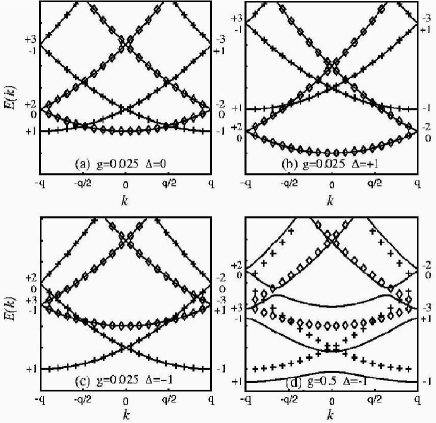
Figure 1: The lowest lying bands of the Hamiltonian given by Eq. (3) for the first Brillouin zone. The dressed energy bands are marked on the $y$-axis with the dominant bare state index $\mu$. Crosses shows the bare energy bands for excited states $|+\rangle$ and diamonds bands for ground bare states $|-\rangle$. In the last figure (d), the coupling is so strong that the bare and dressed energies starts differ considerable. The parameters are given on top of each figure.

In order to solve the problem numerically, the Hamiltonian has to be truncated at some dimension $n$. For small $k$ and relatively low bands, this $n$ should be chosen odd, in order to be consistent with coupling to equal number of states in both ’directions’ from a given initial state. For $n=1$, we obtain the bare eigenenergy, for $n=3$, the bare state $|\psi_{0}^{k}\rangle$ couples to the states $|\psi_{\pm 1}^{k}\rangle$ and so on. In Figs. 1 (a)-(d) we show the lowest-lying bands for the first Brillouin zone, obtained numerically with $n=201$, for the parameters (a) $\Delta=0$, (b) $\Delta=1$ and (c) and (d) $\Delta=-1$. In (d) the coupling is 20 times as large, making the bare and dressed energies differ significantly. On the $y$-axis the dressed bands are labelled with the corresponding dominant $\mu$-value that the bare eigenenergies would have had in the limit of weak coupling, and diamonds indicate a bare lower state $|-\rangle$ energies and crosses bare states $|+\rangle$ energies. When adding the coupling, the crossings become ’avoided’. Note how the gap size decreases with the band index $\nu$, indicating that the state is more weakly coupled to far-away lying states. The crossings between even-even $\mu$ or odd-odd $\mu$ are called Bragg resonances and between odd-even or even-odd $\mu$ Doppleron resonances dyn4 .

In Fig. 2 we illustrate how the presence of the periodic interaction couples the momentum eigenstates (bare states) into dressed states. In Fig. 2(a), the coefficients for the first four dressed states ($\nu=1,2,3,4$) are plotted as a function of $\mu$ for zero quasi-momentum $k=0$. Note that the solutions are either odd or even in $\mu$ and that only the first one is not ’degenerate’ since all other are centered around a crossing. Figure 2(b) shows the same coefficients for a non-zero quasi-momentum $k_{0}=q/4$, and the solutions are no longer symmetric around $\mu=0$. Note that, if any of the coefficients $c_{\mu}^{\nu}$ (for each $\nu$) in Eq. (10) has an absolute value close to unity, the presence of the periodic coupling only modifies the properties of a bare state without too much coupling to other bare states; this is usually the case away from the crossings.

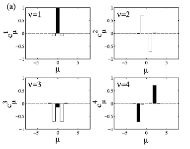
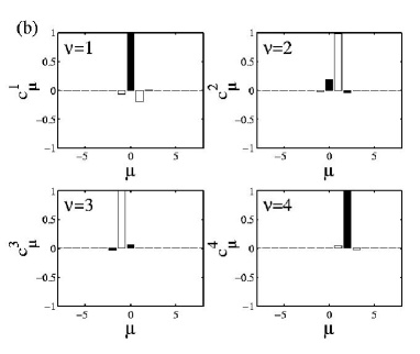
Figure 2: The expansion coefficients $c_{\mu}^{\nu}$ for the four lowest dressed states $\nu=1,2,3,4$, Eq. (10), of bare states $\mu$ for (a) $k=0$ and (b) $k=1/4$. Black bars corresponds to even $\mu$’s with ground state atom, and white bars to odd $\mu$’s with excited atom. The coefficients are symmetric around $\mu=0$ only for $k_{0}=0$. The parameters are in both plots the same as for Fig. 1: $\Delta=0$ and $g_{0}=0.05$.

II.3 Extraction of the effective parameters

We now look for an analytical expression for the energy eigenvalues of the Hamiltonian (11) and for the dispersion curves. Denoting the bare-state energies by

$$\mathcal{E}^{\mu}(k)=\frac{(k+\mu q)^{2}}{2}-(-1)^{\mu}\frac{\Delta}{2},$$ (12)

the energy eigenvalue equation $H|\phi\rangle=E|\phi\rangle$ (for a predefined $k$) can be written as a recursion equation

$$\mathcal{E}^{\mu}c_{\mu}+g(c_{\mu+1}+c_{\mu-1})=Ec_{\mu}.$$ (13)

This equation has, naturally, an infinite number of solutions corresponding to different bands. Truncation of the recursion symmetrically around some index $\nu$ and elimination of the expansion coefficients $c_{\mu}$ yields a continued fraction-like expression

$$\begin{array}[]{ll}E=\mathcal{E}^{\nu}+\frac{g^{2}}{E-\mathcal{E}^{\nu-1}-\frac{g^{2}}{E-\mathcal{E}^{\nu-2}+\frac{g^{2}}{\ldots}}}+\frac{g^{2}}{E-\mathcal{E}^{\nu+1}-\frac{g^{2}}{E-\mathcal{E}^{\nu+2}+\frac{g^{2}}{\ldots}}},\end{array}$$ (14)

which has a form of an iteration equation. We assume that this equation is most applicable in the region where one bare state dominates the dressed state and the truncation of the Hamiltonian (11) or, equivalently, of the recursion equation (13) is performed symmetrically around this state. Note that the truncation of the Hamiltonian is also an effective expansion in the coupling constant $g_{0}$ since, for a small coupling, each base state only couples to a few neighboring bare states while, for a large coupling, many bare states are required to represent a dressed state. This is not, however, true in the vicinity of level crossings where two bare state couple to each other even over many intermediate states.

We illustrate the truncation error with

$$\delta(g_{0},\Delta;n)=|E(k)-E_{n}(k)|,$$ (15)

where $E(k)$ represents the exact dispersion curve and $E_{n}(k)$ the one obtained from a truncated $n\times n$ Hamiltonian. We emphasize that the error depends only on the parameters $g_{0}$ and $\Delta$ due to the chosen length scale; in physical units they both contain the photon wave number since $g_{0}\propto\tilde{g}_{0}/\tilde{q}^{2}$ and $\Delta\propto\tilde{\Delta}/\tilde{q}^{2}$. As already mentioned, we use $q=1$ throughout the paper.

Figure 3 illustrates $\delta(g_{0},\Delta;n)$ as function of $g_{0}$ and $\Delta$, for $k=0$. An almost identical plot of the error is obtained for $k=q/4$, therefore it is omitted. The error increases for large couplings, which is easily understood since a large coupling means that the initial bare state will couple more strongly to other bare states and the dimension of the Hamiltonian must be chosen higher. It is also seen that the increasing detuning $\Delta$, which makes the diagonal elements in the Hamiltonian larger, yields smaller errors.

Figure 3: Error estimate $\delta(g_{0},\Delta;n)$ for $n=5$, as defined in Eq. (15). The quasi-momentum $k=0$. The errors for the $k=1/4$ case is almost identical.

The number of $g_{0}^{2}$-terms included in the continued fraction (14) is related to the truncated size of the Hamiltonian as $(n-1)/2$. Taking any initial value of $E$ and iterating Eq. (14) it is expected that the iteration converges to some eigenvalue $E^{\nu}(k)$ close to the initial value of $E$. For example, for moderate couplings and away from crossings, starting with $E$ coinciding with a bare energy eigenvalue, the iteration is supposed to converge to the corresponding dressed energy eigenenvalue. Thus, analytical approximate results are obtainable by truncation the continued fraction to some $(n-1)/2$ terms and iterate it $j$ times. From numerical investigations of the validity of these two approximations, we draw the conclusion that for certain rangers of the parameters, especially for small couplings $g_{0}$ and large detunings $\Delta\gg 1$, the order of approximation does not need to be very high away from crossings. It has turned out that truncating the Hamiltonian to a $5\times 5$-matrix and iterating the continued fraction (14) twice gives an eigenenergy, which is valid for a large range of parameters. Having an analytical expression for the energy, we can easily calculate the mass parameters. Below we will give only the analytic expression for the case when $k\approx 0$, but the same procedure could be carried out for other cases as well. Since we have assumed $|k|\ll q$, we expand the eigenenergy around $k=0$, but we will also expand the result in powers of $g_{0}^{2}$. The result obtained becomes is given by

$$\begin{array}[]{ccl}E^{(1)}(k)&\approx&-\frac{\Delta}{2}-\frac{4g_{0}^{2}}{q^{2}+2\Delta}+\frac{4\left(7q^{2}-2\Delta\right)g_{0}^{4}}{q^{2}(q^{2}+2\Delta)}+\mathcal{O}(g_{0}^{6})\\ \\ &&+\!\left(\!\frac{1}{2}\!-\!\frac{16q^{2}g_{0}^{2}}{(q^{2}+2\Delta)^{3}}\!+\!\frac{4(111q^{6}-46\Delta q^{4}-28\Delta^{2}q^{2}-8\Delta^{3})g_{0}^{4}}{q^{4}(q^{2}+2\Delta)^{5}}\right.\\ \\ &&+\mathcal{O}(g_{0}^{6})\Big{)}k^{2}+\mathcal{O}(k^{4}).\end{array}$$ (16)

III Propagation of wave packets

In this Section, we analyze the propagation of Gaussian dressed and Gaussian bare states using the effective mass parameters and compare the results with wave function simulations. We also discuss the physical difference of initial bare and dressed states.

Propagation of an initial Gaussian state can be understood in terms of effective parameters, such as the group velocity and the effective mass, which depend on the dispersion curve and are evaluated at the dominant quasi-momentum $k_{0}$ of the wave packet. We assume that the wave packet inside the cavity is initially described by a Gaussian momentum wave function

$$\varphi(k)=\frac{1}{\sqrt[4]{2\pi\Delta_{k}^{2}}}{\rm e}^{-\frac{(k-k_{0})^{2}}{4\Delta_{k}^{2}}}$$ (17)

where $\Delta_{k}$ is the width of the momentum distribution and it is related to the initial width of the position distribution according to $\Delta_{k}=1/(2\pi\Delta_{x})$, whence the initial state is a minimum uncertainty state. Within its range, the energy of the dressed states (belonging to the band $\nu$) can be expanded as

$$\begin{array}[]{cl}E(k)&\approx E(k_{0})+v_{{\rm g}}(k_{0})(k-k_{0})+\frac{1}{2}\frac{1}{m^{*}(k_{0})}(k-k_{0})^{2}\\ \\ &=E_{0}+\frac{1}{2m_{0}(k_{0})}k_{0}^{2}+\frac{1}{m_{1}(k_{0})}k_{0}(k-k_{0})\\ \\ &+\frac{1}{2m_{2}(k_{0})}(k-k_{0})^{2},\end{array}$$ (18)

with $E_{0}=E(k=0)$. We have chosen to use mass parameters for each term in the expansion. Note that, for a free particle, this is merely an expansion of the energy term $E=\frac{1}{2m}k^{2}$ around $k_{0}$, and all the mass parameters $m_{\rm i}$ coincide with the natural mass of the particle.

The three mass parameters in Eq. (18) can now be given the following interpretations: $m_{0}$ yields the energy of a dressed eigenstate as $E(k_{0})-E_{0}=\frac{1}{2m_{0}}k_{0}^{2}$ and, hence, it defines the phase velocity of the dressed state as $v_{p}=E_{0}/k_{0}=\frac{1}{2m_{0}}k_{0}$, $m_{1}$ defines the group-velocity–quasi-momentum relation as $k_{0}=m_{1}v_{{\rm g}}$, and $m_{2}$ determines the mass associated with the wave-packet spreading. Note that, even though we do not consider the case here, $m_{2}$ coincides with the conventional effective mass $m^{*}$ that determines the acceleration caused by an external force acting on the particle wave packet. The first mass parameter $m_{0}$ is, however, nonphysical since its value depends on the choice of zero energy level. It may, however, affect some interference experiment, but we do not consider it here, since it is not expected to effect the propagation. Equation (16) can be used to deduce approximate values for $m_{1}$ and $m_{2}$ near zero-momentum.

III.1 Propagation of Gaussian dressed states

By Gaussian dressed states we mean wave packets centered around the quasi-momentum $k_{0}$, where each wave component belongs to the same energy band of the interacting Hamiltonian,

$$|\Phi_{\nu}(t)\rangle=\int_{-\infty}^{\infty}\varphi(k)|\phi_{\nu}(k)\rangle{\rm e}^{-{\rm i}E^{\nu}(k)t}{\rm d}k.$$ (19)

In principle, the integral should be limited to the first Brillouin zone (or to any one Brillouin zone); in this expression it is assumed that $k_{0}$ is sufficiently far from its boundaries so that the momentum distribution $\varphi(k)$ is negligible outside the zone.

With the use of the expansion of the dressed states in terms of bare states, Eq. (10), and of the integral equality

$$\begin{array}[]{c}\int_{-\infty}^{\infty}\varphi(k)\,{\rm e}^{{\rm i}(kx-E_{\nu}(k)t)}\,{\rm d}k\\ \\ \approx\frac{1}{\sqrt[4]{2\pi\left(\frac{1}{2\Delta_{k}}+\frac{{\rm i}\Delta_{k}t}{m_{2}}\right)^{2}}}{\rm e}^{-\frac{{\left(x-v_{{\rm g}}t\right)}^{2}\,}{4\left(\frac{1}{4\Delta_{k}^{2}}+\frac{{\rm i}t}{2m_{2}}\right)}}{\rm e}^{{\rm i}(k_{0}x-E(k_{0})t)}\end{array}$$ (20)

(the approximate value derives from neglecting higher terms in Eq. (18)), the Gaussian dressed states evolve in time as

$$\begin{array}[]{cc}|\Phi_{\nu}(t)\rangle&=\frac{1}{\sqrt[4]{2\pi\left(\frac{1}{2\Delta_{k}}+\frac{{\rm i}\Delta_{k}t}{m_{2}}\right)^{2}}}{\rm e}^{-\frac{{\left(x-v_{{\rm g}}t\right)}^{2}\,}{4\left(\frac{1}{4\Delta_{k}^{2}}+\frac{{\rm i}t}{2m_{2}}\right)}}|\phi_{\nu}(k_{0})\rangle\end{array}$$ (21)

and has the time-dependent width $\Delta_{x}(t)=|\frac{1}{2\Delta_{k}}+\frac{{\rm i}\Delta_{k}t}{m_{2}}|$. Here we have further assumed that the expansion coefficients $c_{\mu}^{\nu}(k)$ remain constant within the Gaussian momentum distribution. Inclusion of a correction term $c_{\mu}^{\nu}(k)\approx c_{\mu}^{\nu}(k_{0})+d_{\mu}^{\nu}(k_{0})(k-k_{0})$ gives rise to an additional term in the integral, but it still has a Gaussian envelope moving with the same group velocity. In Figs. 4 (a) and (b) we show the propagation of initial Gaussian dressed and bare states. The dressed state stays approximately Gaussian throughout the evolution, while the initial bare state splits up in three main sub-packets corresponding to the bare states $|-,k_{0}\rangle$, $|+,k_{0}-q\rangle$ and $|+,k_{0}+q\rangle$. In order to prepare the initial dressed states, the coupling amplitude is taken to be time dependent $g_{0}(t)$ and is turned on adiabatically from $g_{0}=0$ up to the final value $g_{0}(t)=g_{0}$. In that way, the state remains dressed during the turn-on assuming an adiabatic switch on. As $g_{0}(t)$ has reached the final value $g_{0}$, the wave packet has already broadened, so after the preparation process we do no longer have $\Delta_{x}=1/(2\Delta_{k})$. The numerical method used for wave packet simulations will be discussed in Section III.3.

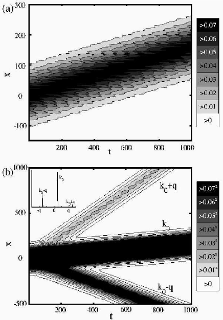
Figure 4: The evolution of (a) an initial Gaussian dressed state and (b) an initial Gaussian bare state. The dressed state stays localized around an average position, while the bare state clearly splits up. The three sub-packets in (b) correspond to the bare states $|-,k_{0}\rangle$, $|+,k_{0}-q\rangle$ and $|+,k_{0}+q\rangle$, which is also seen in the inset showing the final momentum distribution $|\langle k|\Psi\rangle|^{2}$. The parameters are the same in both plots, $g_{0}=0.001$, $\Delta=0$, $x_{0}=0$, $k_{0}=1/4$ and $\Delta_{k}^{2}=1/10000$, and in (b) the atom is initially in its lower state. The contour-bar shows relative values.

III.2 Comparison between bare and dressed states

While in most experimental situations an atom enters a cavity in a well-defined bare state, the mass parameters defined above characterize a dressed state and are not directly applicable. We introduce therefore the overlap (often called Fidelity) between bare and dressed states

$$F^{\nu,\mu}(k)=|\langle\psi_{\mu}^{k}|\phi_{\nu}^{k}\rangle|^{2},$$ (22)

which is the same as the absolute square of the coefficients $c_{\mu}^{\nu}$ in Eq. (10) For a relative small coupling and away from crossings, it is clear which bare state $|\psi_{\mu}^{k}\rangle$ has the largest overlap with a given dressed state $|\phi_{\nu}^{k}\rangle$. However, near crossings two bare states will become important, but still it is easy to decide which ones. Note that, given a quasi-momentum $k$, the crossings depend on the parameter $\Delta$, and the fidelity will change drastically around some particular value on $\Delta$, see Fig. 1. For example, picking $k=q/4$ and $\Delta=0$, the largest overlap with the dressed state with $\nu=1$ is assumed to be with the $\mu=0$ bare state, assuming a small coupling $g_{0}$, while for $-3q^{2}/4<\Delta<-q^{2}/4$ the largest overlap is expected for the $\mu=-1$ bare state.

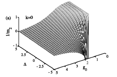
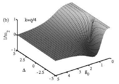
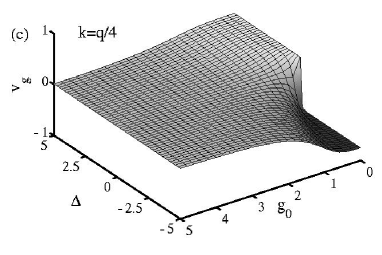
Figure 5: The scale mass parameters $1/(m_{2})$ and $v_{{\rm g}}=k_{0}/m_{1}$ as functions of $g_{0}$ and $\Delta$. The first two plots (a) and (b) show $1/(m_{2})$ for $k=0$ and $k=q/4$, respectively, and (c) the group velocity $v_{{\rm g}}$ for $k=q/4$, where the unperturbed velocity ($g_{0}=0$) should be $v_{0}=1/4$. The result derives from numerical diagonalization of the matrix (11) and numerical calculation of the coefficients of the dispersion curve around the point $k$ of interest. The bare energies of states $\mu=0,-1$ cross for $\Delta=kq-q^{2}/2$ and the dominant bare states of the lowest band changes. This leads to a drastic change in the effective parameters, as seen in the figures.

In Fig. 5 we display the coefficients $m/(m_{2})$ and $v_{{\rm g}}=k_{0}/m_{1}$ as function of $g_{0}$ and $\Delta$. In Figs. 5 (a) and (b) $1/(m_{2})$ is shown for $k=0$ and $k_{0}=1/4$ respectively, and in Fig. 5(c) the group velocity is plotted for $k=1/4$.

From Fig. 5, it is clear that $1/(m_{2})$ differs considerably from the unperturbed value $m=1$. It is now of interest to see how well the corresponding bare and dressed states overlap for the same parameter rangers. We calculate the overlaps $F^{\nu=1,\mu=0}(k=0)$ and $F^{\nu=1,\mu=0}(k=q/4)$ for the two examples. The results are plotted in Figs. 6(a) and (b). As justified earlier, a small coupling increases the overlap. Note that there are ranges where the masses $m_{1}$ (or $v_{{\rm g}}$) and $m_{2}$ are shifted significantly from the free mass $m$ and still the overlap is large, meaning that an initial Gaussian bare state should evolve approximately freely with mass parameters $m_{1}$ and $m_{2}$. In the wave packet simulations below it will be shown that the shifted masses can be observed also for propagating bare states.

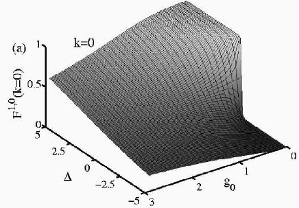
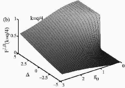
Figure 6: The variation of the overlap (a) $F^{1,0}(0)$ and (b) $F^{1,0}(q/4)$, as defined in Eq. (22), with respect to $g_{0}$ and $\Delta=0$. For positive $k$, a huge change in the overlap occurs when $\Delta=kq-q^{2}/2$, which was also seen in the previous figure of the mass parameters. For such $\Delta$, the corresponding quasi-momentum $k$ is located at a gap, and as $\Delta$ changes more, the lowest dressed states $\nu=1$ will have a larger overlap with bare states with $\mu=\pm 1$ rather than $\mu=0$. This can be clearly understood from Fig. 1 (b) and (c). The photon momentum $q$, which was used to define the characteristic length scale, is, as earlier 1.

III.3 State propagation simulations

Independently of the chosen basis (bare or dressed states), the time evolution of the atom-cavity system is governed by a time-independent Hamiltonian $H=p^{2}/(2m)+V(x)$; with an initial state $|\Psi(t=0)\rangle$ it is written as

$$|\Psi(t)\rangle={\rm e}^{-{\rm i}Ht}|\Psi(t=0)\rangle.$$ (23)

For an $x$-dependent potential $V(x)$, we find, in general, that the kinetic energy term of the Hamiltonian does not commute with the potential. The exponential can therefore not be separated into one momentum exponential and one spatial exponential. However, if the time of propagation $\delta t$ is chosen sufficiently small, the error of splitting up the exponential becomes negligible

$$|\Psi(t+\delta t)\rangle\approx{\rm e}^{-{\rm i}\frac{p^{2}}{2m}\delta t}{\rm e}^{-{\rm i}V(x)\delta t}|\Psi(t)\rangle.$$ (24)

This is called the split operator method, see Ref. split , and the procedure goes as follows: Starting with some state $|\Psi(0)\rangle$ in the $x$-representation, we multiply it by the exponential $\exp(-{\rm i}V(x)\delta t)$, we then take the Fourier transform of the state and obtain it in the $p$-representation, and then we multiply it by $\exp\left[-{\rm i}p^{2}\delta t/(2m)\right]$, and finally transform it back to the $x$-representation with the inverse Fourier transform, which gives us $|\Psi(\delta t)\rangle$. Repeating this $N$ times we obtain $|\Psi(t)\rangle$, for $t=N\delta t$.

For the system considered here, the kinetic and potential terms are

$$\begin{array}[]{ccc}E_{\rm kin}&=\frac{p^{2}}{2}\left[\begin{array}[]{cc}1&0\\ 0&1\end{array}\right]\\ \\ V(x)&=\left[\begin{array}[]{cc}\frac{\Delta}{2}&g(x)\\ g(x)&-\frac{\Delta}{2}\end{array}\right].\end{array}$$ (25)

If the atom is initially in a bare state corresponding to the internal state $|-\rangle$, the wave function is

$$|\Psi(t=0)\rangle=\left[\begin{array}[]{c}0\\ \int dk\,\varphi(k)|k\rangle\end{array}\right]$$ (26)

while, for an initial dressed state, it is given by Eq.(19) for $t=0$.

III.4 Propagation within the cavity

For a given $k_{0}$, the properties of the dispersion curve, and hence of the mass parameters, depend on the physical parameters of the system. From Eq. (16), it is expected that effects are largest for $\Delta=0$ as long as $k_{0}$ is far from a crossing, and thus we choose $\Delta=0$ in the analysis below. Furthermore, we choose to calculate the quantities for $k_{0}=0$ and $k_{0}=q/4$ in the lowest band $\nu=1$.

We will, in this Subsection, show numerical simulations and calculations of the effective parameters for a Gaussian wave packet inside a cavity, but first we investigate the evolution of a bare Gaussian wave packet that is prepared inside the cavity with a momentum $k_{0}=q/2$, corresponding to a gap. At an energy gap, the dispersion curve has a vanishing first order derivative. Hence, if the wave packet has a large overlap with the corresponding dressed states, its group velocity is close to zero. In the weak coupling limit, the time dependent bare state can be expressed in terms of dressed states approximately as

$$\begin{array}[]{ccl}|\psi(t,k_{0}=0.5)\rangle&\approx&\frac{1}{\sqrt{2}}\left({\rm e}^{-{\rm i}E^{\nu=1}t}|\phi_{1}(k_{0}=q/2)\rangle\right.\\ \\ &&+\left.{\rm e}^{-{\rm i}E^{\nu=2}t}|\phi_{2}(k_{0}=q/2)\rangle\right),\end{array}$$ (27)

and using that the gap size is approximately $2g_{0}$ it follows

$$\begin{array}[]{ccl}|\psi(t,k_{0}=q/2)\rangle&\approx&\frac{1}{\sqrt{2}}\left({\rm e}^{i{\rm}g_{0}t}|\phi_{1}(k_{0}=q/2)\rangle\right.\\ \\ &&+\left.{\rm e}^{-{\rm i}g_{0}t}|\phi_{2}(k_{0}=q/2)\rangle\right){\rm e}^{-{\rm i}\mathcal{E}^{0}t}.\end{array}$$ (28)

Thus, the bare state wave packet is supposed to oscillate between upper and lower states $|\pm\rangle$. Figure 7 shows the evolution of such a prepared state. The upper figure shows the wave packets in the $x$-representation for upper, lower and combined internal states, while the lower plot displays the momentum packets.

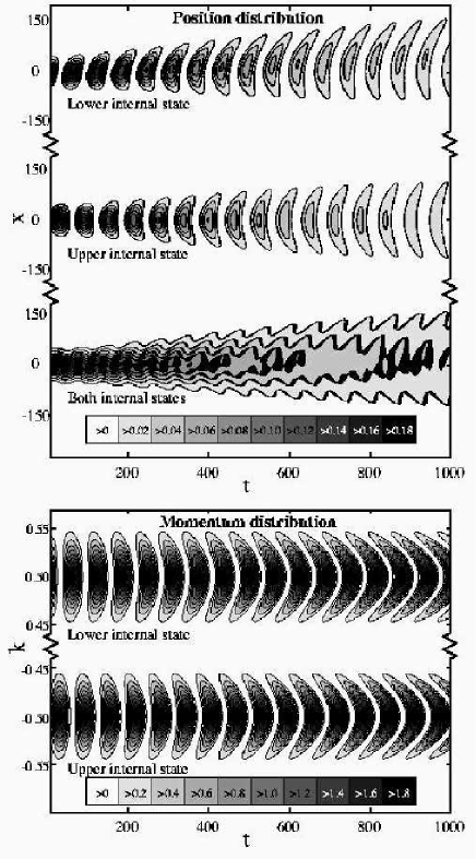
Figure 7: The evolution of an initial Gaussian bare wave packet prepared inside the cavity with $\Delta_{x}^{2}=500$ and $k_{0}=1/2$, corresponding to a quasi-momentum of the first forbidden energy gap. The upper plot shows the wave packets of the ground, excited and total (ground plus excited) atomic state in the $x$-representation. The lower figure displays the wave packet of the ground and excited atomic state in the momentum $k$-representation. It is clear that we have a spreading in $x$ and also a small drift of the lower atomic wave packet. The population ’Rabi’ oscillates between the two states with a period $T_{R}\approx\pi/g_{0}$, corresponding to the $2\pi$ divided by the energy gap size $2g_{0}$ in first order. The remaining parameters are $\Delta=0$ and $g_{0}=0.05$. The contour-bars gives the relative values.

When the atom propagates inside an infinite cavity, it should be possible to describe the atomic wave packet as a freely evolving particle with effective mass parameters defined in Eq. (18), which will be analyzed next. The time of flight $t_{\rm f}$ between $x_{0}$ and $x_{\rm f}$ is given by

$$t_{\rm f}=\frac{x_{\rm f}-x_{0}}{v_{{\rm g}}}=\frac{m_{1}}{m}\frac{(x_{\rm f}-x_{0})}{v_{\rm initial}},$$ (29)

where $v_{\rm initial}$ is the velocity of the atom in absence of the cavity interaction. We will simulate propagation of both bare and dressed wave packets. In the simulation of bare state propagation we use averages, for the atomic state of interest, that is for the wave packet of the ground state, $\langle x\rangle=\frac{\langle-|x|-\rangle}{\langle-|-\rangle}$, in other words we select the wave packet of the ground state $|-\rangle$ and normalize it and then calculate the averages. Physically that assumes that a projective measurement is carried out on the lower state before that position measurement is done. For the dressed states the averages are calculated for the whole atomic wave packet and no projective measurement is assumed. We propagate the initial wave packet from a certain $\langle x_{0}\rangle$ for a time $t_{\rm f}$ and calculate the final average position $\langle x_{\rm f}\rangle$, and deduce the propagation velocity $v=\frac{\langle x_{{\rm f}}\rangle-\langle x_{0}\rangle}{t_{{\rm f}}}$, which should coincide with the group velocity $v_{{\rm g}}=k_{0}/m_{1}$. We use the parameters of one of the previous examples, $\Delta=0$, $\Delta_{x}^{2}=2500$ and $k_{0}=q/4$, but vary the coupling strength $g_{0}$; the final time is taken to be $t_{\rm f}=1000$. During the adiabatic preparation, the dressed wave packet will already broaden, whence its initial width is no longer $\Delta_{x}^{2}=2500$, but this is not expected to affect the group velocity. In Fig. 8 we compare propagation velocities for dressed and bare states with the group velocity obtained from the Floquet theory. The three curves coincide rather well, but, for the case of initial bare state, the agreement is good only for the lower initial state $|-\rangle$, as described above. The whole atomic wave packet, containing both upper and lower atomic states, gives a value $\langle x_{{\rm f}}\rangle$ different from the one using just one atomic state. Thus, we emphasize again that, extracting the propagation velocity with the bare states assumes that the position measurement is carried out for the atom in its lower state, in other words, some of the outcomes will fail, namely when the atom is measured while being excited. The slight difference between dressed state propagation and the Floquet theory might be due to non-adiabatic generation of the initial dressed state.

This scheme clearly gives a good measure of the group velocity and from that it is possible to calculate the mass $m_{1}$.

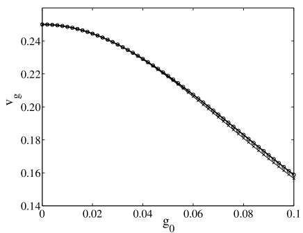
Figure 8: The group velocity $v_{{\rm g}}$ as function of the coupling, obtained, both from the wave packet simulation, circles shows the result from bare state propagation and crosses from dressed state propagation, and the Floquet theory (solid line), when $k_{0}=q/4$. A clear agreement is seen, but unexpectedly the bare state result coincide better with the Floquet one, which might be due to a not fully adiabatic preparation of the dressed state. The parameters are $t_{\rm f}=1000$, $\Delta=0$ and $\Delta_{x}^{2}=2500$.

The mass parameter $m_{2}$, enters the wave packet dynamics through the broadening of the Gaussian dressed state according to

$$\Delta_{x}^{2}(t)=\langle x^{2}\rangle=\frac{1}{4\Delta_{k}^{2}}+\left(\frac{\Delta_{k}}{m_{2}}\right)^{2}t^{2}.$$ (30)

Initial Gaussian bare states do not, however, remain Guassian but split into several wave packets, corresponding to a number of dressed states. In Fig. 4 (b) the initial bare state splits into three main wave packets and, even though the two outer ones may be small, they contribute significantly to the variance since they are far from the center packet. Thus, for the calculation of the bare state variance, the packets in the tails $|x|>150$, which mostly corresponds to excited atomic states, are excluded when $\langle x^{2}\rangle$ is calculated. In Fig. 9 the mass $m_{2}$ is displayed as function of $g_{0}$. The time of propagation is $t_{{\rm f}}=10$, and the mass is obtained by a least square fit of Eq. (30), knowing $\Delta_{x}^{2}(t)$ and $t$. Note that when we prepare the Gaussian dressed states by an adiabatic turn on of the coupling amplitude, Eq. (30) is valid, but the mass $m_{2}$ is not constant during the turn-on, which must be taken into account. This is carried out by assuming a constant coupling amplitude, adjusted by introducing an effective turn-on time $t_{{\rm eff}}$. Thus Eq. (30) becomes

$$\Delta_{x}^{2}(t)=\frac{1}{4\Delta_{k}^{2}}+\left(\frac{\Delta_{k}}{m_{2}}\right)^{2}(t_{{\rm eff}}+t)^{2},$$ (31)

where the mass $m_{2}$ is now constant during the turn-on process. In lowest order, the mass $m_{2}$ behaves as $\propto g_{0}^{2}$, according to Eq. (16), which is indicated in Fig. 9 and it has been confirmed by a polynomial fit to the data, where the dominant coefficient is the one of $g_{0}^{2}$.

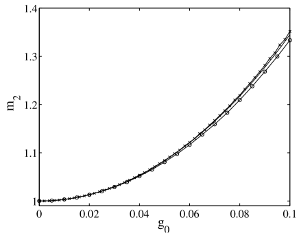
Figure 9: The effective mass $m_{2}$ as function of the coupling, obtained, both from the wave packet simulation of bare (circles) and dressed states (crosses) and the Floquet theory (solid line), when $k=0$. The main reason for the deviation of the result of the bare state propagation is that the wave packet of the lower atomic state, which is used in the calculation, does not stay Gaussian and the tails of the distribution are cut off for $|x|>15$ in the calculation of $\Delta_{x}^{2}$. The parameters are $t_{\rm f}=1000$, $\Delta=0$ and $\Delta_{x}^{2}=1500$.

The measurements of the masses proposed in this Subsection may be used for state preparation. The masses are functions of $g_{0}$, $\Delta$ and $q$ for the one excitation case, but in general it is a function of the effective coupling $g_{0}\sqrt{n}$, where $n$ is the photon number, instead of $g_{0}$. Thus, for a general initial state of the cavity field, a perfect mass measurement will give $m_{1,2}=m_{1,2}(g_{0}\sqrt{n},\Delta,q)$ for any $n$. Only masses $m_{1,2}(g_{0}\sqrt{n},\Delta,q)$ with $n$’s that has a non-vanishing probability from the initial photon distribution, can be detected. Knowing $m_{1}$ or $m_{2}$ and $g_{0}$, $\Delta$ and $q$ it is possible to solve for $n$, meaning that measuring the mass reduces the field to the Fock state $|n\rangle$, a sort of projective measurement. Physically this means that an initial state $|\Phi(t=0)\rangle$ splits up in a set of states $|\Phi(t)\rangle_{n}$ for the various photon numbers $n$. If all overlaps between different final states $|\Phi(t)\rangle_{n}$ vanish it is possible to separate the individual parts with one single measurement. However, having non-overlapping final states seems unlikely in realistic experiments.

III.5 Scattering and transmission

In order to simulate atomic scattering and transmission by the cavity, the mode function coupling $g(x)$ needs to be modified by multiplication of an envelope function

$$\bar{g}=\frac{1}{2}\left[\tanh\left(\frac{x+x_{{\rm l}}}{x_{{\rm e}}}\right)-\tanh\left(\frac{x-x_{{\rm l}}}{x_{{\rm e}}}\right)\right].$$ (32)

This function goes to zero for large $|x|$ and is centered around $x=0$, the cavity length is given by $2x_{{\rm l}}$, and the ’slope’ how fast it turns on/off is determined by $x_{{\rm e}}$. Thus, the coupling will approximately be zero for $x<-x_{{\rm l}}$ and $x>x_{{\rm l}}$, and in the interval $[-x_{{\rm l}},x_{{\rm l}}]$ it behaves as $g(x)=2g_{0}\cos(qx)$. We choose $x_{{\rm l}}$ such that $2x_{{\rm l}}\ll\lambda=2\pi/q$, and $x_{{\rm e}}$ such that the coupling is turned on/off smoothly, but fast enough for a non-adiabatic transition. The envelope function allows us to test boundary effects from not having a completely periodic potential; it turns out, however, that the dynamics follows very well the Floquet predictions as long as $\lambda\ll 2x_{{\rm l}}$.

An incoming atom entering a cavity has been studied in a series of papers refl1 ; refl2 ; refl3 , were, in particular, the transmission and reflection coefficients have been calculated. In these papers, either a mesa function or a hyperbolic secant squared coupling $g(x)$ was used to obtain analytical solutions. The spatial wave function was assumed to be a plane wave and not a propagating wave packet. In the case of a mesa function or a hyperbolic secant, the atom effectively sees a potential barrier or a well with an amplitude $\pm\sqrt{\Delta^{2}/4+g^{2}(x)n}$, where $n$ is the photon number. The case of a standing wave shape of the coupling is, however, different; the spectrum of allowed energies is then formed by bands, with forbidden gaps in between. Thus, an atom entering the cavity mode must have an allowed energy in order to traverse the cavity. If the atom has an energy falling into forbidden energy gaps, it must be reflected (assuming the tunneling rate through the cavity to be negligible).

Going back to Fig. 1, we see that, when $\Delta=0$, the crossings occur for $(\mu+1/2)q$ and $\mu q$, where, as before, $\mu=0,\pm 1,\pm 2,...\,$ . We know that these become avoided crossings when the coupling is turned on, and they give the forbidden energy gaps in the spectrum. The gap size decreases for increasing band index $\nu$, and the largest gap is at $k=\pm q/2$ between the first two bands. If the momentum distribution $\varphi(k)$ of the incident atom is such that $\langle k\rangle\approx 0.5q$ and the energy spread, due to the spread $\Delta k$, is smaller than the gap width, the atom should be reflected when it approaches the cavity mode, and from energy conservation we must have $\langle k\rangle\approx 0.5q\,\Rightarrow\langle k\rangle\approx-0.5q$. The atom thus shifts the momentum by one unit $q$ and, due to the form of the Hamiltonian (3), also the internal atomic-cavity state flips. Hence the quantum state is changed, by the reflection against the lowest gap, as

$$\int\,dk\,\varphi(k)|k\rangle|\pm\rangle\,\,\Rightarrow\,\,\int\,dk\,\varphi(k)|k-q\rangle|\mp\rangle.$$ (33)

On the other hand, the internal atomic state will not flip for scattering against a gap corresponding to momentum $\mu q$. If the atom goes from $|\uparrow\rangle$ ($|\downarrow\rangle$) to $|\downarrow\rangle$ ($|\uparrow\rangle$), the photon number must also change as $n\rightarrow n\pm 1$. This means, for example, that starting with the vacuum and reflecting $N$ excited atoms from the cavity allows one to create an $N$-photon Fock state in the mode. If instead the atoms scatter when they are initially in their ground state, the mode will be cooled down towards lower photon numbers.

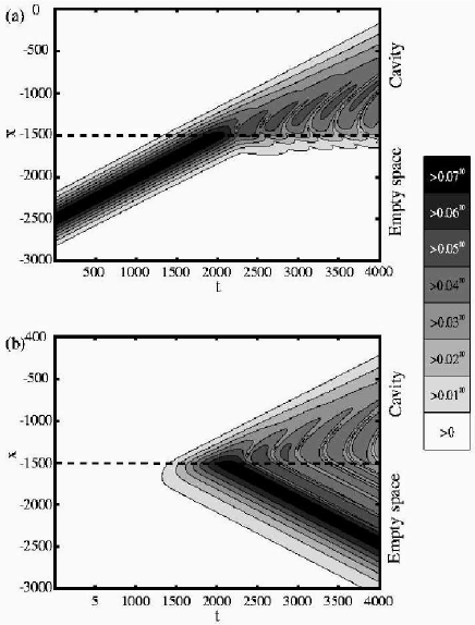
Figure 10: Scattering of an atom against a cavity. The cavity is located within $|x|\lesssim x_{{\rm l}}$ for $x_{{\rm l}}=1500$ (marked with dashed line) and $x_{{\rm e}}=50$. In (a) we show the ground state atomic wave function $|\langle-|\langle x|\Psi\rangle|^{2}$ and in (b) the upper state $|\langle+|\langle x|\Psi\rangle|^{2}$ as function of position $x$ and time $t$. Note that the atom starts to propagate in its lower state at $x_{0}=-2500$ at the time $t=0$ with momentum $k_{0}=q/2$ until it reaches the cavity boundary at $x=-1500$. It is reflected and its internal state is flipped to the upper state $|\uparrow\rangle$. The reflection is due to the fact that its energy coincides with an energy gap; hence the atom absorbs the photon from the cavity field and the impact changes the direction of propagation. Note the scale of the contours, which indicate that almost everything is reflected, as confirmed in Fig. 13 for the atomic inversion. The parameters are here are $g_{0}=0.01$, $\Delta=0$, and $\Delta_{x}^{2}=2500$. The contour-bar shows relative values.

Figure 10 shows the results of a numerical simulation, in which an atom reflects from a cavity. The atom is initially in its lower atomic state $|-\rangle$ and ends up in $|+\rangle$. The cavity starts at around $x=-150$ and ends at $x=150$, $x_{{\rm l}}=1500$ and $x_{{\rm e}}=50$, and the flip takes place at the edge of the cavity. The scale of the contours is chosen such that even the small amplitudes of the wave packet is seen; a closer look on the scale indicates that almost all the population is reflected.

If the energy spread of the incident atom is broader than the band gap, the tails of the packet are in the allowed region of energies, and can therefore enter the cavity. Figure 11 depicts the same system as Fig. 10, but the momentum distribution is much wider, hence part of the wave packet is transmitted. This phenomenon can also be observed on the momentum representation of the wave packet: The part of the wave packet having allowed energies is transmitted, while the forbidden part is reflected, with a flipped atomic state $|\downarrow\rangle\rightarrow|\uparrow\rangle$. Thus, due to the forbidden energies, a ’hole’ is seen in the momentum distribution. This suggests a way of measuring the band/gap structure, since the energies of the reflected atoms correspond to gaps. The momentum wave packet for the $|-\rangle$ atomic state is shown in Fig. 12. We observe that the momenta close to $k=q/2$ are ’burned out’.

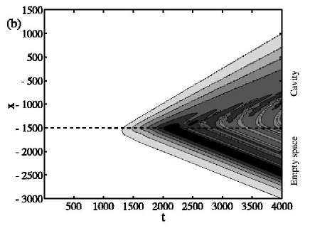
Figure 11: This figure shows the same as Figs. 10 (a) and (b), except that now the momentum distribution is much wider, $\Delta_{x}^{2}$ is chosen 100 instead of 2500 as in the previous plot. The consequence is that energy spread exceeds the band gap and the tails of the momentum wave packet are transmitted rather than reflected. The contour scale is the same as in Fig. 10, and a closer look shows that a much larger part of the wave packet is propagating inside the cavity. Note how the wave packets spreads much faster in these plots.

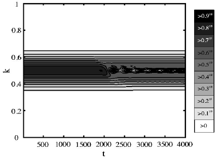
Figure 12: The momentum distribution of the lower atomic state, $|\langle-|\langle k|\Psi\rangle|^{2}$, corresponding to Fig. 11, as a function of time $t$. The forbidden energies are ’burned out’ when the packet hits the cavity. The contour-bar gives relative values.

The atomic inversion, defined as $\langle\sigma_{3}\rangle$, indicates the amount of the atomic population that is in the upper respectively the lower state. If $\langle\sigma_{3}\rangle=-1$, all the population is in the lower state, while if $\langle\sigma_{3}\rangle=1$, the atom is completely excited. In Fig. 13 we show the inversion for the two examples above, $\Delta_{x}^{2}=2500$ and $\Delta_{x}^{2}=100$, as function of time. Here it is obvious that, in the first case, almost the entire population is flipped, while in the second most of it is not flipped. We note that, after the atomic wave packet has reached the cavity, an oscillating behavior can be observed. The reason is the interference between the dressed states involved.

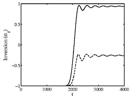
Figure 13: The atomic inversion $\langle\sigma_{3}\rangle$ as function of time $t$ for the example in the previous Fig. 10 (solid line), and Fig. 11 (dashed line). It is clear that at the cavity boundary, the atom flips from $|\downarrow\rangle$ to $|\uparrow\rangle$ in the first example, but when the momentum width becomes larger than the gap, parts of the wave packet will not be reflected and therefore will not be flipped.

So far the atom has entered the cavity with a momentum $\langle k\rangle$ that lies within a band gap, but we now consider the situation in which it is within the first allowed band $\nu=1$. We still choose the atom to start in its ground state $|-\rangle$, but now with $k_{0}=q/4$, halfway between $k=0$ and the gap at $k=0.5q$. If the overlap between the initial bare state and the dressed state $|\phi^{k}_{1}\rangle$ is close to unity, the population of the internal states of the system stays approximately constant, and the atom will traverse the cavity without changing between its two states $|\uparrow\rangle$ and $|\downarrow\rangle$ nor change its momentum state. It will, however, experience a shift in the masses $m_{1}$ and $m_{2}$. The overlap for these parameters is $F^{\nu=1,\mu=0}(k_{0}=1/4)=0.998$, which is close to 1. The result of the simulation is given in Fig. 14. The atomic inversion is shown in Fig. 15, from which we see that $\sim 99.8\,\,\%$ of the population is in the lower state during der the situation in which it is within the first allowed band the time inside the cavity, as predicted by the overlap. After leaving the cavity, the atom regains its original internal and momentum state.

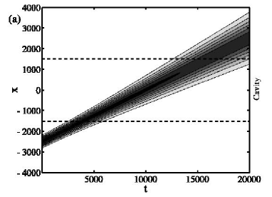
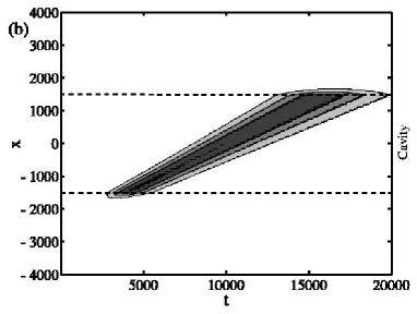
Figure 14: Transmission of the atom through the cavity. The plots are the same as in Figs. 10(a) and (b), but now the initial momentum is $k_{0}=q/4$, and the atom energy falls on the first allowed energy band, contrary to Figs. 10 and 11. The overlap between the initial bare state $|\Psi_{0}^{k_{0}=1/4}\rangle$ and the dressed state $|\phi_{1}^{k_{0}=1/4}\rangle$ is 0.998. Thus, the propagation can be described using the effective parameters and the wave packet remains Gaussian; only a small amount of population is transferred into the $|+\rangle$-state and the Gaussian wave packet spreads according to the effective mass $m_{2}$ and traverse the cavity with a velocity $v_{{\rm g}}$. The contour scale is the same as in Fig. 10 and the cavity boundaries are marked by the dashed lines.

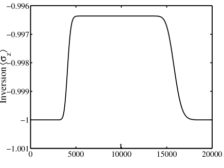
Figure 15: The atomic inversion $\langle\sigma_{z}\rangle$, corresponding to Fig. 14. Note that when the atom has traversed the cavity, it regains its original state. The asymmetry is due to broadening of the wave packet while traversing the cavity, leading to a longer transit time as it leaves the cavity compared to when it enters.

As mentioned above, scattering $N$ excited atoms against an initially empty cavity, so that they are all reflected in the lower state, creates a Fock state with exactly $N$ photons. Other interesting situations may be realized as well with the same idea. Assuming the cavity to be empty from the beginning and the atom in some linear combination of upper and lower state and with a momentum corresponding to the first gap, the state evolves as

$$\Big{(}a|\uparrow\rangle+b|\downarrow\rangle\Big{)}|q/2\rangle|0\rangle\,\Rightarrow\,\Big{(}a|-q/2,1\rangle+b|q/2,0\rangle\Big{)}|\downarrow\rangle.$$ (34)

Since a lower state atom will traverse unaffected through the cavity, while the upper state atom is reflected, this is realizing an atomic ’Stern-Gerlach’ type of measurement. If instead, the field is initially in some linear combination of vacuum and the one photon state and the atom in the lower state it follows that

$$|\downarrow,q/2\rangle\Big{(}a|0\rangle+b|1\rangle\Big{)}\,\Rightarrow\,\Big{(}a|\downarrow,q/2\rangle+b|\uparrow,-q/2\rangle\Big{)}|0\rangle.$$ (35)

Thus a photon ’Stern-Gerlach’ type of measurement is realized, assuming that the field is restricted to the states $|0\rangle$ and $|1\rangle$. Obviously, the scheme may not be used only for separating atomic or field stats, but it works also as a model for creating entanglement between the involved degrees of freedom, momentum, atomic and field states.

IV Conclusion

We have analyzed theoretically the problem of a two-level atom propagating within a quantized standing wave electromagnetic field, with an emphasis on the mass parameters in atomic cavity QED systems. We have approached the problem with two different strategies: the Floquet theory for the periodic Hamilton operator, and the wave packet simulations. The first is a purely mathematical procedure, which offers numerical and approximate analytic expressions for the mass parameters, while the second is a more physical attack. The analytic results offer a hint of the dependence of the masses on the physical parameters. Roughly speaking, a small detuning $\Delta$, small photon momentum $q$, and a large atom-field coupling $g_{0}$ yield large mass shifts.

The dynamics of an atomic wave packet inside (or entering) the cavity can be understood in terms of the dispersion curve $E^{\nu}(k)$, where $k$ is the quasi-momentum of a generalized plane wave and $\nu$ is the band index. In the Taylor expansion around some quasi-momentum $k_{0}$ each term defines a mass paramter; in this paper we have considered the mass $m_{1}=\hbar k_{0}/v_{{\rm g}}$ related to the group velocity $v_{{\rm g}}$ of Gaussian wave packets and the mass $m_{2}$ associated with the spreading of the wave packet:

$$\frac{1}{m_{1}}=\left.\frac{1}{\hbar^{2}k_{0}}\frac{\partial E^{\nu}(k)}{\partial k}\right|_{k=k_{0}}\,\mathrm{and}\,\,\,\frac{1}{m_{2}}=\frac{1}{\hbar^{2}}\left.\frac{\partial^{2}E^{\nu}(k)}{\partial k^{2}}\right|_{k=k_{0}}.$$ (36)

Note that $m_{2}$ is the same as the customary effective mass $m^{*}$ introduced to describe, for example, acceleration of electrons within a crystal under an external force. These parameters vary essentially over different scales of the coupling, as seen in Fig. 5. Even an arbitrary small coupling $g$ results in strong effects in the atomic dynamics. For $g\geq\frac{1}{2}$, both the group velocity and $1/m_{2}$ approaches zero and finally saturates towards this value, which in unscaled quantities can be written as

$$E_{\rm int}=\hbar\tilde{g}\leq\frac{\hbar^{2}\tilde{q}^{2}}{2m}=E_{\rm kin}.$$ (37)

Hence, whenever the characteristic interaction energy exceeds the characteristic kinetic energy of the lowest band, the band is essentially flat and the energy becomes nearly independent of the quasi-momentum. Using typical values $\lambda=1000$ nm. and $m=100$ a.m.u. we get a characteristic time scale $T_{s}\sim 0.4$ $\mu s.$ giving us the unscaled coupling $\tilde{g}=g/T_{s}\approx 10$ kHz for saturation. Note that dividing our dimensionless detuning $\Delta$ and the coupling $g$ by $T_{s}$ gives real physical quantities.

The effective masses are only defined for dressed states with well defined momenta, and in many situations, the system starts out in a bare state. It is, however, possible that the bare states have a large overlap with some dressed state and may be assigned an effective mass. This has been investigated in great detail in the present paper and numerical simulation of propagation for both Gaussian dressed and Gaussian bare states has been analyzed and compared with both each other and with results given by the Floquet theory. Both the group velocity and the effective mass $m_{2}$ have been extracted numerically in the various cases with a good agreement as compared with the values obtained from the Floquet theory.

In most experiments today, the atom and field are prepared separately and the atom is shot through the cavity with a preselected velocity. The state of the complete system is then, most likely, not in a dressed state, but rather a bare state. We have not, in the text, discussed in detail how one may prepare initial dressed states. A standard method is to use a slow adiabatic change of some external controllable parameter. For the JC model, bare and dressed states becomes identical in the two limits $g_{0}\rightarrow 0$ or $\Delta\rightarrow\pm\infty$. By letting the atom traverse a Fabry-Perot cavity almost perpendicular to the standing wave mode it is possible to have very small initial atomic velocities $\hbar k_{0}/m$ along the standing wave mode even for not so cold atoms by varying the angle of injection; the atoms will have a high transverse velocity and a slow velocity in the $x$-direction along the standing wave mode. Thus, it is enough to quantize the atomic motion in just the $x$-direction, while the $y$ and $z$-directions are treated classically. In the case of a Fabry-Perot cavity, the transverse Gaussian mode shapes can then be described by the time envelope $\exp(-t^{2}/\Delta t^{2})$. If the turn-on of the transverse Gaussian mode is slow enough, the atom will traverse the cavity in a dressed state. Another feasible way to prepare the dressed states is to use an external ion trap to confine the ion inside an off-resonance cavity, and then slowly tune the cavity into resonance and shut off the external trap.

In addition to investigating the dynamics of the atom in the presence of the standing wave mode, we have suggested various applications for state preparations and measurements. It has been explained and shown numerically how an incident atom may be reflected by the cavity while simultaneously leaving one photon into it, which might be used for creation of Fock states. The model can also be used for ’Stern-Gerlach’ type of measurements, separating the upper and lower atomic states spatially. Likewise, it could also be used for separating the vacuum $|0\rangle$ from the one photon state $|1\rangle$ and to create various entangled states, like EPR-states.

The paper is purely theoretical, and we understand that experimental measurement of the effective masses will pose several challenges, depending on the approach chosen. First of all, the nodes of a free-space standing wave have a tendency to drift, which is avoided in a natural way by using an optical or a microwave cavity. Both regimes, however, bring new difficulties: A periodic field mode is needed in order to observe changes predicted in the propagation characteristics; present high-Q microwave cavities have, unfortunately, dimensions of the order of wavelength. Hence the optical wave number is not well defined and the Floquet approach adapted in this paper is no longer applicable microwave . In the optical regime, time scales of both the atomic spontaneous emission and the cavity decay are usually shorter than the interaction time, and both processes will strongly affect the atom-cavity system in a way that is not included in the present consideration. One way to go around these difficulties is to use extremely long lived transitions and configurations in which upper atomic levels are only slightly populated, cf. Figs. 5 and 6; the cavity decay may be circumvented by using a driven cavity, hence rendering the light field effectively classical. Similar experiments are performed using classical laser fields made stable by a set of mirrors, see e.g. bloch . The same kind of setup could in principle be used for determination of the effective mass and one may then neglect decay of the field. The dynamics of the atom will then be the same when it interacts with a classical field as with a Fock state.

The Floquet approach presented for the description of atomic motion in terms of an effective mass parameters is, in principle, independent of weather the two-level atom interacts with a classical light field or with a photonic Fock state of a quantised field. The present results may, however, not be realistically achievable in today’s cavity QED systems. Our treatment does set the stage for the concept of an electromagnetic effective mass and we may only hope that novel experimental conditions will, one day, make possible the observation of cavity-induced mass modification.

References

- (1) Cavity Quantum Electrodynamics, Advances in Atomic, Molecular and Optical Physics, edited by P.R. Berman (New york, Academic Press, 1994)
- (2) E.T. Jaynes and F.W. Cummings, Proc. IEEE, 51, 89 (1963).
- (3) B.W. Shore and P.L. Knight, J. Mod. Opt. 40, 1195 (1993).
- (4) A. Rauschenbeutel, G. Nogues, S. Osnaghi, P. Bertet, M. Brune, J.M. Raimond and S. Haroche, Phys. Rev. Lett. 83, 5166 (1999).
- (5) S.B. Zheng and G.C. Guo, Phys. Rev. Lett. 85, 2392 (2000).
- (6) L.M. Duan, A. Kuzmich and H.J. Kimble, Phys. Rev. A 67, 032305 (2003).
- (7) J. Larson and B.M. Garraway, J. Mod. Opt. 51, 1691 (2004).
- (8) H. Walther, J. Mod. Opt. 51, 1859 (2004).
- (9) M. Brune, E. Hagley, J. Dreyer, X. Maitre, A. Maali, C. Wunderlich, J.M. Raimond and S. Haroche, Phys. Rev. Lett. 77, 4887 (1996).
- (10) M.O. Scully, G.M. Meyer and H. Walther, Phys. Rev. Lett. 76, 4144 (1996).
- (11) G.M. Meyer, M.O. Scully and H. Walther, Phys. Rev. A 56, 4142 (1997).
- (12) B.G. Englert, J. Schwinger, A.O. Barut and M.O. Scully, Europhys. Lett. 14, 25 (1991).
- (13) M. Löffler, G.M Meyer, M. Schröder, M.O. Scully and H. Walther, Phys. Rev. A 56, 4153 (1997).
- (14) R. Arun and G.S. Agarwal, Phys. Rev. A 64, 065802 (2001).
- (15) S. Haroche, M. Brune and J.M. Raimond, Europhys. Lett. 14, 19 (1991).
- (16) P.W.H. Pinkse, T. Fisher, P. Maunz and G. Rempe, Nature 404, 365 (2000).
- (17) C.J. Hood, T.W. Lynn, A.C. Doherty, A.S. Parkins and H.J. Kimble, Science 287, 1447 (2000).
- (18) A.C. Doherty, T.W. Lynn, C.J. Hood and H.J. Kimble, Phys. Rev. A 63, 013401 (2000).
- (19) J. Ye, D.W. Vernooy and H.J. Kimble, Phys. Rev. Lett. 83, 4987 (1999).
- (20) C. Schön and J.I. Cirac, Phya. Rev. A 67, 043813 (2003).
- (21) P. Horak, G. Hechenblaikner, K.M. Gheri, H. Stecher and H. Ritsch, Phys. Rev. Lett. 79, 4974 (1997).
- (22) D.W. Vernooy and H.J. Kimble, Phys. Rev. A 56, 4287 (1997).
- (23) A.B. Mundt, A. Kreuter, C. Becher, D. Leibfried, J. Eschner, F. Schmidt-Kaler and R. Blatt, Phys. Rev. Lett. 89, 103001 (2002).
- (24) W. Ren and H.J. Carmichael, Phys. Rev. A 51, 752 (1995).
- (25) J.T. Zhang, X.L Feng, W.Q. Zhang and Z.Z. Xu, Chin. Phys. Lett. 19, 670 (2002).
- (26) Y.T. Chough, S.H. Youn, H. Nha, S.W. Kim and K. An, Phys. Rev. A 65, 023810 (2002).
- (27) M. Wilkens, E. Schumacher and P. Meystre, Phys. Rev. A 44, 3130 (1991).
- (28) I. Cusumano, A. Vaglica and G. Vetri, Phys. Rev. A 66, 043408 (2002).
- (29) C.J. Hood, M.S. Chapman, T.W. Lynn and H.J. Kimble, Phys. Rev. Lett. 80, 4157 (1998).
- (30) F. Saif, F. LeKien and M.S. Zubairy, Phys. Rev. A 64, 043812 (2001).
- (31) G. Compagno, J.S. Peng and F. Persico, Phys. Rev. A 26, 2065 (1982).
- (32) A.Z. Muradyan and G.A. Muradyan, J. Phys. B 35, 3995 (2002).
- (33) A. Vaglica, Phys. Rev. A 52, 2319 (1995).
- (34) A.M. Herkommer, V.M. Akulin and W.P. Schleich, Phys. Rev. Lett. 69, 3298 (1992).
- (35) M.J. Holland, D.F. Walls and P. Zoller, Phys. Rev. Lett. 67, 1716 (1991).
- (36) P. Storey, M. Collett and D. Walls, Phys. Rev. Lett. 68, 472 (1992).
- (37) R. P. Feyman, Statistical Mechanics, (Addison Wesley, 1990).
- (38) C. Kittel, Quantum Theory of Solids, (New York, Wiley, 1987).
- (39) J. Larson and S. Stenholm, J. Mod. Opt. 50, 2705 (2003).
- (40) R.R. Schlicher. Opt. Commun. 70, 97 (1988).
- (41) A.C. Doherty, A.S. Parkins, S.M. Tan and D.F. Walls, Phys. Rev. A 57, 4804 (1998).
- (42) T. Sleator and M. Wilkens, Phys. Rev. A 48, 3286 (1993).
- (43) Handbook of Mathematical Functions, Natl. Bur. Stand. Appl. Math. Ser. No. 55, edited by M. Abramowitz and I.A. Stegun (U.S. GPO, Washington, DC, 1972).
- (44) A. R. Kolovsky, J. Opt. B 4, 218 (2002).
- (45) E. Arimondo, A. Bambini and S. Stenholm, Phys. Rev. A 24, 898 (1981).
- (46) M.D. Fleit, J.A. Fleck, and A. Steiger, J. Comp. Phys. 81, 412 (1982).
- (47) M. Brune, E. Hagley, J. Dreyer, X. Maitre, A. Maali, C. Wunderlich, J.M. Raimond and S. Haroche, Phys. Rev. Lett. 77, 4887 (1996).
- (48) D. Meschede, H. Walther, and G. Müller, Phys. Rev. Lett. 54, 551 (1985).
- (49) Q. Niu, X-G. Zhao, G. A. Georgakis, and M. G. Raizen, Phys. Rev. Lett. 76, 4504 (1996).