Combinatorial approach to generalized Bell and Stirling numbers and boson normal ordering problem

Abstract

We consider the numbers arising in the problem of normal ordering of expressions in boson creation $a^{\dagger}$ and annihilation $a$ operators ($[a,a^{\dagger}]=1$). We treat a general form of a boson string $(a^{\dagger})^{r_{n}}a^{s_{n}}...(a^{\dagger})^{r_{2}}a^{s_{2}}(a^{\dagger})^{r_{1}}a^{s_{1}}$ which is shown to be associated with generalizations of Stirling and Bell numbers. The recurrence relations and closed-form expressions (Dobiński-type formulas) are obtained for these quantities by both algebraic and combinatorial methods. By extensive use of methods of combinatorial analysis we prove the equivalence of the aforementioned problem to the enumeration of special families of graphs. This link provides a combinatorial interpretation of the numbers arising in this normal ordering problem.

, ,

1 Introduction

In this paper we consider a pair of boson creation $a^{\dagger}$ and annihilation $a$ operators satisfying the commutation relation

$$[a,a^{\dagger}]=1.$$ (1)

These operators play a fundamental role in the formalism of second quantization in Quantum Mechanics and Quantum Field Theory (QFT) [1],[2],[3]. Since the creation and annihilation operators do not commute serious problems with their ordering arise. A very convenient and well defined form of the operators depending on $a$ and $a^{\dagger}$ is the so called normally ordered form [4]. An operator is said to be in a normally ordered form if all creation operators stand to the left of the annihilation operators. The most important application field of the normal order is the QFT [3]. For a recent study of the interplay of the QFT, normal order and combinatorics see Ref.[5]. Procedure of normal ordering of the operator, i.e. moving all the creation operators to the left with the use of relation Eq.(1), is in general a nontrivial task. A first example is ordering of the power of the number operator [6][7]:

$$(a^{\dagger}a)^{n}=\sum_{k=1}^{n}S(n,k)(a^{\dagger})^{k}a^{k},$$ (2)

where $S(n,k)$ are the Stirling numbers of the second kind [8] enumerating partitions of the set of $n$ elements into $k$ nonempty subsets, and satisfying the following recurrence relation $S(n+1,k)=S(n,k-1)+kS(n,k)$ with initial values $S(n,n)=S(n,1)=1$.
As the extension of this result we have considered operators in the form $(a^{\dagger})^{r}a^{s}$ ($r$, $s$ -positive integers, $r\geq s$), for which a normally ordered form is given by

$$[(a^{\dagger})^{r}a^{s}]^{n}=(a^{\dagger})^{n(r-s)}\sum_{k=s}^{ns}S_{r,s}(n,k)(a^{\dagger})^{k}a^{k},$$ (3)

where $S_{r,s}(n,k)$ are generalized Stirling numbers [9],[10],[11],[12],[13],[14]. This kind of formulas allow one to write the exponentials $e^{\lambda(a^{\dagger})^{r}a^{s}}$ in the normally ordered form and then easily calculate the coherent state expectation values which are of importance e.g. in Quantum Optics [4]. The clue of these calculations is the knowledge of the properties of the numbers $S_{r,s}(n,k)$. As they are of a combinatorial origin, the recurrence relations, Dobiński-type formulas, closed-form expresions and generating functions were extensively studied [10].
In the following we further extend these results to normal ordering of a general boson string in the form $(a^{\dagger})^{r_{n}}a^{s_{n}}\dots(a^{\dagger})^{r_{2}}a^{s_{2}}(a^{\dagger})^{r_{1}}a^{s_{1}}$, by establishing a link to special structures in enumerative combinatorics. This in turn gives us the rigorous demonstration of the properties of the generalized Stirling and Bell numbers arising in this problem. The construction of the graphs (the so called ’bugs’) associated with these numbers provides a graphical interpretation of the normal ordering procedure.

2 Generalized Bell and Stirling numbers

In this section we define the generalization of ordinary Bell and Stirling numbers which arise in the solution of the normal ordering problem for a boson string. Given two sequences of positive integers ${\mathbf{r}}=(r_{1},r_{2},\dots,r_{n})$ and ${\mathbf{s}}=(s_{1},s_{2},\dots,s_{n})$ we let $S_{{\mathbf{r}},{\mathbf{s}}}(k)$ be the positive integers appearing in the expansion

$$(a^{\dagger})^{r_{n}}a^{s_{n}}\dots(a^{\dagger})^{r_{2}}a^{s_{2}}(a^{\dagger})^{r_{1}}a^{s_{1}}=(a^{\dagger})^{d_{n}}\sum_{k=s_{1}}^{s_{1}+s_{2}+\dots+s_{n}}S_{{\mathbf{r}},{\mathbf{s}}}(k)(a^{\dagger})^{k}a^{k},$$ (4)

where $d_{n}=\sum_{i=1}^{n}(r_{i}-s_{i})$, which we assume here to be non-negative. We observe that the whole theory can be carried through for $d_{n}$ negative, at the cost of minor adaptations, which however do not change the numbers involved. Note that the r.h.s. of Eq.(4) is already normally ordered.
We call $S_{{\mathbf{r}},{\mathbf{s}}}(k)$ the generalized Stirling numbers of the second kind. The generalized Bell number is defined as the sum

$$B_{{\mathbf{r}},{\mathbf{s}}}=\sum_{k=s_{1}}^{s_{1}+s_{2}+\dots+s_{n}}S_{{\mathbf{r}},{\mathbf{s}}}(k).$$ (5)

In this notation the generalized Stirling numbers defined in Eq.(3) correspond to a uniform case ${\mathbf{r}}=\overbrace{(r,r,\dots,r)}^{n}$ and ${\mathbf{s}}=\overbrace{(s,s_{,}\dots,s)}^{n}$.
We introduce the notation ${\mathbf{r}}\ \uplus\ r_{n+1}=(r_{1},r_{2},\dots,r_{n},r_{n+1})$ and ${\mathbf{s}}\ \uplus\ s_{n+1}=(s_{1},s_{2},\dots,s_{n},s_{n+1})$ and state the recurrence relation satisfied by generalized Stirling numbers $S_{{\mathbf{r}},{\mathbf{s}}}(k)$

$$S_{{\mathbf{r}}\uplus r_{n+1},{\mathbf{s}}\uplus s_{n+1}}(k)=\sum_{j=0}^{s_{n+1}}\left(\!\!\!\begin{array}[]{c}s_{n+1}\\ j\end{array}\!\!\!\right)(d_{n}+k-j)_{s_{n+1}-j}S_{{\mathbf{r}},{\mathbf{s}}}(k-j),$$ (8)

where $(l)_{p}=l\cdot(l-1)\cdot...\cdot(l-p+1)$ is the falling factorial.
One can give the derivation of Eq.(8) by induction using the following consequence of Eq.(1) (see the proof in [2]):

$$a^{k}(a^{\dagger})^{l}=\sum_{p=0}^{k}\left(\!\!\begin{array}[]{c}k\\ p\end{array}\!\!\right)(l)_{p}(a^{\dagger})^{l-p}a^{k-p}.$$ (11)

The full details of this approach can be consulted in [14].
Observe that the problem stated above can also be formulated in terms of the multiplication $X$ and derivative $D$ operators as they satisfy $[D,X]=1$. The representation of boson commutation relation with the $D$ and $X$ operators resembles the Bargmann representation [4], used in connection with coherent states. (Here we do not enter into that framework, with all the intricacies of the scalar product, hermiticity etc., as in our context only the algebraic properties matter.) Then Eq.(4) can be rewritten as:

$$X^{r_{n}}D^{s_{n}}\dots X^{r_{2}}D^{s_{2}}X^{r_{1}}D^{s_{1}}=X^{d_{n}}\sum_{k=s_{1}}^{s_{1}+s_{2}+\dots+s_{n}}S_{{\mathbf{r}},{\mathbf{s}}}(k)X^{k}D^{k}.$$ (12)

Acting with both sides of Eq.(12) on the exponential function $e^{x}$ we get the identity

$$X^{r_{n}}D^{s_{n}}\dots X^{r_{2}}D^{s_{2}}X^{r_{1}}D^{s_{1}}e^{x}=x^{d_{n}}e^{x}B_{{\mathbf{r}},{\mathbf{s}}}(x)$$ (13)

where

$$B_{{\mathbf{r}},{\mathbf{s}}}(x)=\sum_{k=s_{1}}^{s_{1}+s_{2}+\dots+s_{n}}S_{{\mathbf{r}},{\mathbf{s}}}(k)x^{k}$$ (14)

is the so called generalized Bell polynomial. Observe that the order of the so defined generalized Bell polynomial does not depend on ${\mathbf{r}}$. Eq.(13) gives the formula

$$X^{d_{n+1}}e^{x}B_{{\mathbf{r}}\uplus r_{n+1},{\mathbf{s}}\uplus s_{n+1}}(x) = X^{r_{n+1}}D^{s_{n+1}}e^{x}x^{d_{n}}B_{{\mathbf{r}},{\mathbf{s}}}(x).$$ (15)

Using the well known commutation rule (equivalent to the Leibniz rule) $D^{n}e^{x}f(x)=e^{x}(D+I)^{n}f(x)$ we get the recursive formula

$$B_{{\mathbf{r}}\uplus r_{n+1},{\mathbf{s}}\uplus s_{n+1}}(x)=X^{s_{n+1}-d_{n}}(D+I)^{s_{n+1}}X^{d_{n}}B_{{\mathbf{r}},{\mathbf{s}}}(x)$$ (16)

By taking coefficients of $x^{k}$ on both sides of Eq.(16) we obtain the recurrence relation for the generalized Stirling numbers of Eq.(8).
Observe that the action of the l.h.s. of Eq.(12) on $e^{x}$ may be calculated explicitly. To this end one first evaluates it on the monomial $x^{n}$ yielding $\left[\prod_{j=1}^{n}(d_{j-1}+n)_{s_{j}}\right]x^{n+d_{n}}$ which in turn easily gives the result of the action on the exponential function $e^{x}$.
With this observation, together with Eq.(13) we arrive at the extended Dobiński-type relation for generalized Bell polynomials

$$B_{{\mathbf{r}},{\mathbf{s}}}(x)=e^{-x}\sum_{m=s_{1}}^{\infty}\left[\prod_{j=1}^{n}(m+d_{j-1})_{s_{j}}\right]\frac{x^{m}}{m!},$$ (17)

which by Cauchy’s multiplication of series yields the expression for $S_{{\mathbf{r}},{\mathbf{s}}}(k)$:

$$S_{{\mathbf{r}},{\mathbf{s}}}(k)=\frac{1}{k!}\sum_{m=0}^{k}\left(\!\!\!\begin{array}[]{c}k\\ m\end{array}\!\!\!\right)(-1)^{k-m}.\prod_{j=1}^{n}(m+d_{j-1})_{s_{j}}$$ (18)

An alternative, very similar demonstration of the above results can be carried through with the use of coherent states. These are defined for complex $z$, as $|z\rangle=e^{-|z|^{2}/2}\sum_{n=0}^{\infty}\frac{z^{n}}{\sqrt{n!}}|n\rangle$, where $a^{\dagger}a|n\rangle=n|n\rangle$, $a|z\rangle=z|z\rangle$ and $\langle n|n^{\prime}\rangle=\delta_{n,n^{\prime}}$ [4]. The $|n\rangle$’s are called the number states. The coherent state matrix element of Eq.(4) establishes a link to generalized Bell polynomials of Eq.(14):

$$\langle z|(a^{\dagger})^{r_{n}}a^{s_{n}}\dots(a^{\dagger})^{r_{2}}a^{s_{2}}(a^{\dagger})^{r_{1}}a^{s_{1}}|z\rangle=(z^{*})^{d_{n}}B_{{\mathbf{r}},{\mathbf{s}}}(|z|^{2}),$$ (19)

which after some algebra, provides an equivalent derivation of Eqs.(17) and (18). The first instance where the relation between the coherent state matrix elements and the Bell polynomials appears is Ref.[7], again for the generic case of Eq.(2), for which conventional Bell polynomials are obtained.
We shall proceed now to give a combinatorial interpretation of the above results. The essence of subsequent paragraphs will be a graph-theoretical description of the problem. We define the structures (graphs) that are counted by the generalized Bell and Stirling numbers and then give a thorough combinatorial derivation of the recurrence relations, Dobiński-type formulas and other closed-form expressions. The Eqs.(8), (17) and (18) will emerge from purely combinatorial considerations and this will permit the bijective identification of algebraic and combinatorial structures.

3 Bugs, colonies, settlements and recurrence relations

We introduce now a number of tools needed to describe the problem in the graph-theoretical language.

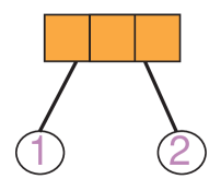
Figure 1: A $(3,2)$-bug

Definition 3.1

A bug of type $(r,s)$ consists of a body and $s$ legs. The body is formed by $r$ linearly ordered empty cells. Each foot of the $s$ legs is labelled with one number from an integer segment $(m,m+s]:=\{m+1,m+2,\dots,m+s\}$, see Fig.1.

Definition 3.2

Consider a set of $n$ bugs, the first one of type $(r_{1},s_{1})$ and feet-labelled with labels in $(0,s_{1}]$, the second of type $(r_{2},s_{2})$ with labels in $(s_{1},s_{1}+s_{2}]$ and so on. A colony is one of the possible ways of organizing the bugs using the following procedure. The first bug has to stand over the ground. Once the $(j-1)$th bug is placed, the $j$th is placed by putting some (or none) of its $s_{j}$ feet in the ground and each one of the rest in one of the empty cells of the bodies of the preceding bugs, see Fig.2. The pair of sequences $({\mathbf{r}},{\mathbf{s}})$, ${\mathbf{r}}=(r_{1},r_{2},\dots,r_{n})$, ${\mathbf{s}}=(s_{1},s_{2},\dots,s_{n})$, carrying the information about the types of the bugs is called the type of the colony. The legs of the colony standing on the ground are called free.
Assume now that there is a set of $m$ empty cells in the ground. An $m$-settlement is a colony where each one of the feet corresponding to the free legs is placed in one of the ground cells. A surjective settlement is one where all the ground cells are occupied. The type of a settlement is defined to be the type of the subjacent colony.

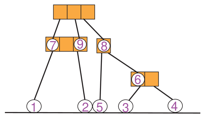
Figure 2: A colony of type (3,2,1,3;2,2,2,3) and $5$ free legs.

The main theorem of interest for us is:

Theorem 3.1

The Stirling number $S_{{\mathbf{r}},{\mathbf{s}}}(k)$, $s_{1}\leq k\leq s_{1}+s_{2}+\dots+s_{n}$, counts the number of colonies of type $({\mathbf{r}},{\mathbf{s}})$ having exactly $k$ free legs. The Bell number $B_{{\mathbf{r}},{\mathbf{s}}}$ counts the number of colonies of type $({\mathbf{r}},{\mathbf{s}})$.

Before proving it, we state the following

Lemma 3.1

A colony of type $({\mathbf{r}},{\mathbf{s}})$ and with $k$ free legs has exactly $d_{n}+k$ empty cells.

Proof. The total number of cells of the colony is equal to $\sum_{i=1}^{n}r_{i}$. The number of occupied cells is equal to the total number of legs minus the number of free legs ($\sum_{i=1}^{n}s_{i}-k$). $\Box$
Now we are ready to prove the Theorem 3.1.
Proof. Denote by $C_{\mathbf{r},\mathbf{s}}(k)$ the number of colonies of type $(\mathbf{r},\mathbf{s})$ with exactly $k$ free legs. Since $C_{(r_{1};s_{1})}(k)=S_{(r_{1};s_{1})}(k)=\delta(s_{1},k)$ it is enough to prove that the numbers $C_{\mathbf{r},\mathbf{s}}(k)$ satisfy the same recursion as the generalized Stirling numbers of Eq.(8).

$$C_{{\mathbf{r}}\uplus r_{n+1},{\mathbf{s}}\uplus s_{n+1}}(k)=\sum_{j=0}^{s_{n+1}}\left(\!\!\!\begin{array}[]{c}s_{n+1}\\ j\end{array}\!\!\!\right)(d_{n}+k-j)_{s_{n+1}-j}\ C_{{\mathbf{r}},{\mathbf{s}}}(k-j)$$ (20)

The l.h.s. is the number of colonies of type $({\mathbf{r}}\uplus r_{n+1},{\mathbf{s}}\uplus s_{n+1})$ having exactly $k$ free legs. We claim that in the right hand side the expression

$$\left(\!\!\!\begin{array}[]{c}s_{n+1}\\ j\end{array}\!\!\!\right)(d_{n}+k-j)_{s_{n+1}-j}\ C_{{\mathbf{r}},{\mathbf{s}}}(k-j)$$

gives the number of such colonies where the $(n+1)$th bug has exactly $j$ free legs. Obviously, this would prove the identity. We now prove our claim. In order to get a colony with $k$ free legs the $(n+1)$th bug has to be placed in a colony of type $({\mathbf{r}},{\mathbf{s}})$ and $k-j$ free legs. $C_{{\mathbf{r}},{\mathbf{s}}}(k-j)$ is the number of such colonies. We choose the free legs of the $(n+1)$th bug in $\left(\!\!\!\begin{array}[]{c}s_{n+1}\\ j\end{array}\!\!\!\right)$ ways. Since by proposition (3.1) there are $d_{n}+k-j$ empty cells in the $n$-bugs colony, $(d_{n}+k-j)_{s_{n+1}-j}$ gives the number of ways of distributing the rest of the feet of the $(n+1)$th bug into the empty cells. $\Box$

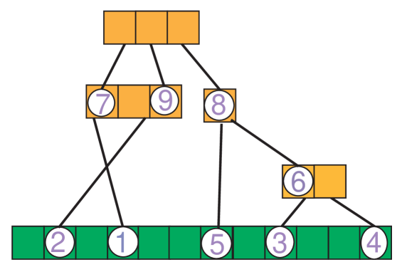
Figure 3: A $12$-settlement of the colony in Fig.(2)

In the next section will follow a number of propositions clarifying the properties of structures in question.

4 Counting settlements and Dobiński-type Relations

We shall count now the number of $m$-settlements which will provide the link with Eqs.(17) and (18) viewed from the combinatorial perspective.

Theorem 4.1

Let $p(m,{\mathbf{r}},{\mathbf{s}})$ be the number of $m$-settlements of type $({\mathbf{r}},{\mathbf{s}})$. We have

$$p(m,{\mathbf{r}},{\mathbf{s}})=\prod_{j=1}^{n}(m+d_{j-1})_{s_{j}}.$$ (21)

Proof. There are $(m)_{s_{1}}$ ways of placing the feet of the first bug into the $m$ ground cells. After placing the $(j-1)$th bug there are $m+d_{j-1}$ empty cells available (the previously placed bugs have provided $\sum_{i=1}^{j-1}r_{i}$ empty cells and occupied $\sum_{i=1}^{j-1}s_{i}$ cells). Then, there are $(m+d_{j-1})_{s_{j}}$ ways of placing the $s_{j}$ feet of the $j$th bug. $\Box$

Corollary 4.1

We have the polynomial identity

$$\prod_{j=1}^{n}(x+d_{j-1})_{s_{j}}=\sum_{k=s_{1}}^{s_{1}+s_{2}+\dots+s_{n}}S_{{\mathbf{r}},{\mathbf{s}}}(k)(x)_{k}.$$ (22)

Proof. By the previous theorem, for an integer value of $x$ the l.h.s. counts the number of $x$-settlements of type $({\mathbf{r}},{\mathbf{s}})$. $S_{{\mathbf{r}},{\mathbf{s}}}(k)(x)_{k}$ counts the number of ways of settling a colony of type $({\mathbf{r}},{\mathbf{s}})$ with $k$ free legs in $x$ ground cells. Then, the r.h.s. is another way of counting $x$-settlements. $\Box$
The exponential generating function of the surjective settlements is equal to the polynomials

$$B_{{\mathbf{r}},{\mathbf{s}}}(x)=\sum_{k=s_{1}}^{s_{1}+s_{2}+\dots+s_{n}}S_{{\mathbf{r}},{\mathbf{s}}}(k)k!\frac{x^{k}}{k!}=\sum_{k=s_{1}}^{s_{1}+s_{2}+\dots+s_{n}}S_{{\mathbf{r}},{\mathbf{s}}}(k)x^{k}.$$

Corollary 4.2

(Extended Dobiński-type relations)
We have the identity

$$B_{{\mathbf{r}},{\mathbf{s}}}(x)e^{x}=\sum_{m=s_{1}}^{\infty}\prod_{j=1}^{n}(m+d_{j-1})_{s_{j}}\frac{x^{m}}{m!}.$$ (23)

Proof. Taking the coefficient of $\frac{x^{m}}{m!}$ of the left hand side we obtain

$$\sum_{k=0}^{m}\left(\!\!\begin{array}[]{c}m\\ k\end{array}\!\!\right)S_{{\mathbf{r}},{\mathbf{s}}}(k)k!=\sum_{k=0}^{m}S_{{\mathbf{r}},{\mathbf{s}}}(k)(m)_{k}.$$

By the previous corollary it is equal to the coefficient of $\frac{x^{m}}{m!}$ in the right hand side. $\Box$
From Eq.(23) we obtain

$$B_{{\mathbf{r}},{\mathbf{s}}}(x)=e^{-x}\sum_{m=s_{1}}^{\infty}\prod_{j=1}^{n}(m+d_{j-1})_{s_{j}}\frac{x^{m}}{m!}$$ (24)

and

$$B_{{\mathbf{r}},{\mathbf{s}}}\equiv B_{{\mathbf{r}},{\mathbf{s}}}(1)=e^{-1}\sum_{m=s_{1}}^{\infty}\frac{1}{m!}\prod_{j=1}^{n}(m+d_{j-1})_{s_{j}}\ .$$ (25)

Taking the coefficient of $\frac{x^{k}}{k!}$ on both sides of equation (24) we obtain the formula for the generalized Stirling numbers

$$S_{{\mathbf{r}},{\mathbf{s}}}(k)=\frac{1}{k!}\sum_{m=0}^{k}\left(\!\!\begin{array}[]{c}k\\ m\end{array}\!\!\right)(-1)^{k-m}\prod_{j=1}^{n}(m+d_{j-1})_{s_{j}}.$$ (26)

Evidently Eq.(24) is identical to Eq.(17) and so are Eqs.(26) and (18). This emphasizes again the already stated bijective correspondence between algebraic and combinatorial structures.

5 Uniform colonies and settlements

A colony or a settlement with all the bugs of the same type is called uniform. A uniform colony with $n$ bugs of type $(r,s)$ is called a colony of type $(r,s)^{n}$. Following the notation of [10] the corresponding Stirling and Bell numbers, enumerating uniform colonies of type $(r,s)^{n}$, are denoted respectively by $S_{r,s}(n,k)$ and $B_{r,s}(n).$ Clearly, for ${\mathbf{r}}=\overbrace{(r,r,\dots,r)}^{n}$ and ${\mathbf{s}}=\overbrace{(s,s_{,}\dots,s)}^{n}$, $S_{r,s}(n,k)=S_{{\mathbf{r}},{\mathbf{s}}}(k)$ and $B_{r,s}(n)=B_{{\mathbf{r}},{\mathbf{s}}}$. The recursive formula, Dobiński-type relations and its consequences appearing here are natural extensions of those investigated in [10].

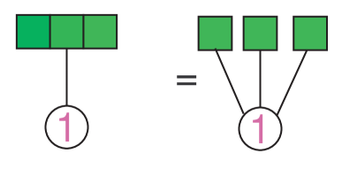
Figure 4: A $(3,1)$-bug and corresponding small planar tree.

The case $s=1$ can be mapped into trees and forests. An $(r,1)$-bug can be identified with a planar tree, i.e. a tree where the leaves are all connected to the root and linearly ordered (see Fig.4). An increasing tree is one where the internal vertices are labelled with labels in a totally ordered set and the labels increase on any path from the root to any internal vertex. The uniform colonies with $s=1$ corresponds to forests of increasing $r$-ary planar trees. The free legs are the roots of the trees (see Fig.5). For $r=1,$ there is only one $1$-ary increasing tree for each $n$. Then $B_{1,1}(n)=B(n)$ is the ordinary Bell number.

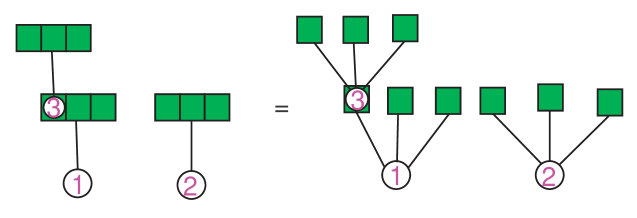
Figure 5: A uniform colony of type $(3,1)^{3}$ and the corresponding forest of increasing trees.

The exponential generating function of the $r$-ary planar increasing trees $T_{r}(x)$ satisfy the differential equation (see [15], Chap. 5) $y^{\prime}=(y)^{r}$. From this we obtain $T_{r}(x)=\sqrt[1-r]{1-(r-1)x},$ for $r>1$. The generalized Bell number $B_{r,1}(n)$ counts the number of $r$-forests with $n$ internal vertices. By the exponential formula we obtain

$$\sum_{n=0}^{\infty}B_{r,1}(n)\frac{x^{n}}{n!}=\exp\{{\sqrt[1-r]{1-(r-1)x}-1}\}.$$ (27)

We quote the explicit expression [10]:

$$B_{r,1}(n)=\frac{(r-1)^{n-1}}{e}\sum_{k=1}^{\infty}\frac{\Gamma(n+\frac{k}{r-1})}{\Gamma(1+\frac{k}{r-1})(k-1)!}.$$ (28)

In a subsequent publication we shall demonstrate that the summation formulas of the type Eq.(28) can be also obtained for many other strings describing the uniform case.

6 Conclusions

We have obtained analytic expressions and combinatorial interpretation of the integers generalizing conventional Bell and Stirling numbers, arising in the normal ordering of a boson string. All of their properties can be interpreted in terms of graph-theoretical language. The proof of the main result may also be obtained with the use of combinatorial theory of species [15],[16],[17]. The results constitute an application of combinatorial analysis which produces the solution of quantum mechanical problem of normal ordering. For alternative interpretations of the numbers investigated in this work see Refs.[18] and [19]. It is an outstanding problem how to extend the key results of this work to the boson $q$-analogs. In this respect the Refs.[20],[21] and [22] will be of essential help.

We thank L. Haddad for important discussions.

PB wishes to thank the Polish Ministry of Scientific Research and Information Technology for support under Grant no: 1P03B 051 26.

References

References

- [1] J. Baez and J. Dolan, From finite sets to Feynman diagrams, in Mathematics Unlimited - 2001 and Beyond, vol. 1, Eds. Björn Engquist and Wilfried Schmid, (Springer, Berlin, 2001) p. 29
- [2] W. H. Louisell, Quantum statistical properties of radiation, (Wiley, New York, 1990)
- [3] M.E. Peshkin and D.V. Schroeder, Introduction to Quantum Field Theory, (Addison Wesley, 1995)
- [4] J.R. Klauder and E.C.G. Sudarshan, Fundamentals of Quantum Optics, (Benjamin, New York, 1968)
- [5] P. Blasiak, K.A. Penson, A.I. Solomon, A. Horzela and G.H.E. Duchamp, Some useful combinatorial formulas for bosonic operators, J. Math. Phys. 46 (1974) 052110
- [6] J. Katriel, Combinatorial aspects of boson algebra, Lett. Nuovo Cim. 10 (1974) 565
- [7] J. Katriel, Bell numbers and coherent states, Phys. Lett. A 237 (2000) 159
- [8] L. Comtet, Advanced Combinatorics, (Reidel, Dordrecht, 1974)
- [9] P. Blasiak, K.A. Penson and A.I. Solomon, The general boson normal ordering problem, Phys. Lett. A 309 (2003) 198
- [10] P. Blasiak, K.A. Penson and A.I. Solomon, The Boson Normal Ordering Problem and Generalized Bell Numbers, Ann. Comb. 7 (2003) 127
-
[11]
P. Blasiak, A. Horzela, K.A. Penson, G.H.E. Duchamp and A.I. Solomon,
Boson Normal Ordering via Substitutions and Sheffer-type Polynomials, Phys. Lett. A 338 (2005) 108
arXiv:quant-ph/0501155 -
[12]
W. Lang, On generalizations of the Stirling number triangles J. Int. Seqs. Article 00.2.4 (2000),
available at http://www.research.att.com/ njas/sequences/JIS/ - [13] M. Schork, On the combinatorics of normal ordering bosonic operators and deformations of it, J. Phys. A: Math. Gen. 36 (2003) 4651
- [14] P. Blasiak, Combinatorics of boson normal ordering and some applications, PhD Thesis University of Paris VI and Polish Academy of Sciences, arXiv:quant-ph/…
- [15] F. Bergeron, G. Labelle, P. Leroux, Combinatorial Species and Tree-like Structures, Encyclopedia of Mathematics and its Applications 67, (Cambridge University Press, 1998)
- [16] A. Joyal, Une théorie combinatoire des séries formelles, Adv. Math. 42 (1981) 1
-
[17]
P. Flajolet and R. Sedgewick, Analytic
Combinatorics - Symbolic Combinatorics, 2005,
Preprint http://algo.inria.fr/flajolet/Publications/books.html - [18] A.I. Solomon, G.H.E. Duchamp, P. Blasiak, A. Horzela and K.A. Penson, Normal Order: Combinatorial Graphs, in 3rd International Symposium on Quantum Theory and Symmetries, Eds. P.C. Argyres et al, (World Scientific Publishing, Singapore, 2004) p.368, arXiv:quant-ph/0402082
- [19] A. Varvak, Rook numbers and the normal ordering problem, in 16th Annual International Conference on Formal Power Series and Algebraic Combinatorics (Vancouver B.C., Canada, 2004) p.259, arXiv:math.CO/0402376
- [20] R. Ehrenborg and M. Readdy, Juggling and applications to -analogues, Discrete Math. 157 (1996) 107
- [21] J. Katriel and M. Kibler, Normal ordering for deformed boson operators and operator-valued deformed Stirling numbers, J. Phys. A: Math. Gen. 25 (1992) 2683
- [22] P. Blasiak, A. Horzela, K.A. Penson and A.I. Solomon, Deformed bosons: Combinatorics of the normal ordering, Czech. J. Phys. 54 (2004) 1185, arXiv:quant-ph/0410226