1 Introduction

The Casimir effect [1] has in recent years attracted a great deal of interest (for recent reviews, see [2, 3, 4, 5]). The advent of accurate experiments has accentuated the need of performing detailed calculations of the Casimir forces, based upon realistic input values for the permittivities in the (assumed homogeneous) materials. In the case of two semi-infinite media separated by a gap $a$ - the standard set-up in the Casimir context - the formula in question is that due to Lifshitz [6]. In the case of a micrometer-sized sphere above a plane substrate - a case that is tractable via use of the proximity force approximation when the spherical surface is weakly curved [7] - the experimental accuracy is claimed in the literature to be on the 1 % level. We shall not here give an overview of recent experiments; we will return to some examples below. The reader may instead consult recent reviews: a detailed exposition on the experiments up to 2001 is given in Bordag et al. [4], a survey of the developments in the last four years is given by Milton [2], section 3.6, and the works of the Purdue group is presented by Decca et al. [8]. (A brief survey of the experiments is given also in the note [9].)

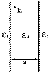
Figure 1: Parallel plate-geometry. The two surfaces are located at $z=0$ and $z=a$.

We shall consider the simple set-up shown in figure 1. There are two metallic semi-infinite media of permittivities $\varepsilon_{1}$ and $\varepsilon_{3}$, with a dielectric medium of permittivity $\varepsilon_{2}$ in between. For simplicity we assume that region 2 is vacuum (air), so that $\varepsilon_{2}=1$. The surfaces are assumed to be perfectly flat, of infinite extension, and the media are assumed nonmagnetic. Our intention is to work out values for the attractive Casimir surface pressure ${\cal F}(a)$ versus gap width $a$ for similar and dissimilar metals, when the temperature $T$ is finite. Of main interest will be the temperature correction, in view of the conflicting opinions in the literature on this point. We will follow the same calculational strategy as in our earlier recent papers on these issues [10, 11, 12].

We shall consider three different metals; gold, copper, and aluminium. For these metals we have access to excellent numerical data for the permittivities (courtesy of Astrid Lambrecht and Serge Reynaud). We know how $\varepsilon(i\zeta)$ varies with imaginary frequency $\zeta$ over seven decades, $\zeta\in[10^{11},10^{18}]$ rad/s, at room temperature. For frequencies up to about $1.5\times 10^{15}$ rad/s the data are nicely reproduced by the Drude dispersion relation

$$\varepsilon(i\zeta)=1+\frac{\omega_{p}^{2}}{\zeta(\zeta+\nu)},$$ (1)

where $\omega_{p}$ is the plasma frequency and $\nu$ the relaxation frequency. For the three metals mentioned we have [13, 14]

$$\omega_{p}=9.0\,{\rm eV},\quad\nu=35\,{\rm meV}\quad{\rm Au}$$

$$\omega_{p}=9.05\,{\rm eV},\quad\nu=30\,{\rm meV}\quad{\rm Cu}$$

$$\omega_{p}=11.5\,{\rm eV},\quad\nu=50\,{\rm meV}\quad{\rm Al}$$ (2)

(note that 1 eV=$1.519\times 10^{15}$ rad/s). Using these data we can calculate the Casimir pressures to an accuracy better than 1%.

We shall consider three different temperatures. First, it is of interest to work out explicitly the zero-temperature Casimir pressure. When discussing finite temperature corrections one should first of all know what is meant by the $T=0$ reference level. This issue is not trivial, since most of the $T=0$ theoretical predictions have been referring to the idealized case where $\varepsilon=\infty$ from the outset. As discussed extensively in earlier works [2, 10, 12, 11], the correct model in an idealized setting is the modified ideal metal (MIM) model, which assumes unit reflection coefficients for all but the transverse electric (TE) zero frequency mode. Our argument rests upon the condition that the relaxation frequency $\nu(0)$ at zero frequency remains different from zero. Here, as in Ref. [11], we will calculate the $T\approx 0$ pressure numerically, inserting real data for $\varepsilon(i\zeta)$. We shall choose $T=1$ K as the lower temperature limit. It turns out that this limit is stable numerically, and numerical trials around this limit indicate that it describes the zero temperature case with good accuracy. This method, although numerically demanding, is physically better than adopting the simple idealized metal model.

The second temperature of interest is room temperature, $T=300$ K. Recognizing that the difference between Casimir pressures at $T=0$ and $T=300$ K will hardly become a measurable quantity we shall instead consider, as our third chosen temperature, $T=350$ K. The difference between the Casimir pressures at the two last-mentioned temperatures will perhaps soon become accessible in experiment. We shall therefore focus upon calculating how this difference varies with $a$.

The present calculations, involving three different metals and three different temperatures, are of interest for comparison of future experimental work on the finite temperature Casimir force. To our knowledge, these are the first calculated results for unequal metal surfaces at finite temperature. We ought here to mention that the first correct calculations of finite temperature Casimir forces between two equal gold, copper, or aluminium metal half planes were made by Boström and Sernelius [15, 16]; these authors considered also two thin equal metal films of gold, silver, copper, beryllium, or tungsten [17, 18]. The calculations by Boström and Sernelius showed that the retarded van der Waals or Casimir interaction in more or less the same separation range (around 1 $\mu$m) as considered in the present paper depends on the choice of material for two equal metal surfaces. The present work is thus a step beyond this in that it considers unequal metal surfaces.

It has repeatedly been pointed out by some authors that our use of the Drude dispersion relation runs into conflict with the Nernst theorem in thermodynamics; cf., for instance, [19, 20]. We have shown earlier, however, that this is not the case [11, 10]. Thus, these thermodynamic issues will not be given further attention here.

In the next section we present the general formalism, for similar as well as for dissimilar media, and give then in section 3 the results of our calculations in several diagrams. With respect to the temperature correction, we restrict ourselves in this section to the difference between $T=0$ and $T=300$ K predictions. In section 4 we focus our attention on the difference between the mentioned 300 K and 350 K cases.

In the main text, we put $\hbar=c=k_{B}=1$.

2 Basic formalism

We consider first the case of two identical media, $\varepsilon_{1}=\varepsilon_{3}\equiv\varepsilon$. With the same notation as in [10, 11] we can write the Casimir pressure as

$${\cal F}=-\frac{1}{\pi\beta a^{3}}{\sum_{m=0}^{\infty}}^{\prime}\int_{m\gamma}^{\infty}y^{2}dy\left[\frac{A_{m}e^{-2y}}{1-A_{m}e^{-2y}}+\frac{B_{m}e^{-2y}}{1-B_{m}e^{-2y}}\right],$$ (3)

where

$$A_{m}=\left(\frac{\varepsilon p-s}{\varepsilon p+s}\right)^{2},\quad B_{m}=\left(\frac{s-p}{s+p}\right)^{2},\quad s=\sqrt{\varepsilon-1+p^{2}},$$

$$p=\frac{q}{\zeta_{m}},\quad y=qa,\quad q=\sqrt{k_{\perp}^{2}+\zeta_{m}^{2}},$$

$$\zeta_{m}=\frac{2\pi m}{\beta},\quad\gamma=\frac{2\pi a}{\beta}.$$ (4)

The prime on the summation sign means that the $m=0$ term is counted with half weight; $\beta=1/T$ is the inverse temperature. The minus sign in Eq. (3) means that the force is attractive.

[The following point should be noted. Assume that a plane wave is incident from the left medium ($z<0$) towards the boundary at $z=0$. For the TM mode, the ratio between the reflected wave amplitude $R^{TM}$ and the incident wave amplitude $A^{TM}$ is equal to the square root of the coefficient $A_{m}$, after the real frequency $\omega$ has been replaced with the imaginary frequency $\zeta$ ($\omega=i\zeta$), corresponding to the surface mode:

$$\frac{R^{TM}}{A^{TM}}=\sqrt{A_{m}}\,;$$ (5)

cf. Appendix B in [10]. Analogously, for the TE mode:

$$\frac{R^{TE}}{A^{TE}}=\sqrt{B_{m}}\,.]$$ (6)

Generalization to the case of dissimilar media leads to the following expression:

$${\cal F}=-\frac{1}{\pi\beta a^{3}}{\sum_{m=0}^{\infty}}^{\prime}\int_{m\gamma}^{\infty}y^{2}dy\left[\frac{\Delta_{1}^{TM}\Delta_{2}^{TM}e^{-2y}}{1-\Delta_{1}^{TM}\Delta_{2}^{TM}e^{-2y}}+\frac{\Delta_{1}^{TE}\Delta_{2}^{TE}e^{-2y}}{1-\Delta_{1}^{TE}\Delta_{2}^{TE}e^{-2y}}\right],$$ (7)

where

$$\Delta_{1}^{TE}=\frac{s_{1}-p}{s_{1}+p},\quad\Delta_{2}^{TE}=\frac{s_{3}-p}{s_{3}+p},$$

$$\Delta_{1}^{TM}=\frac{\varepsilon_{1}p-s_{1}}{\varepsilon_{1}p+s_{1}},\quad\Delta_{2}^{TM}=\frac{\varepsilon_{3}p-s_{3}}{\varepsilon_{3}p+s_{3}}.$$ (8)

Again, if the two media are equal we have $\Delta_{1}=\Delta_{2}$ for each of the modes, so that

$$\Delta_{1}^{TM}\Delta_{2}^{TM}\rightarrow A_{m},\quad\Delta_{1}^{TE}\Delta_{2}^{TE}\rightarrow B_{m},$$ (9)

and the formula (3) is recovered.

We calculate the expression (7) by means of MATLAB. The zero frequency case $m\rightarrow 0$ may be treated separately by analytical methods, at least if we are considering an idealized model for the metal, because in this limit there is an interplay with the other limit $\varepsilon\rightarrow\infty$ in the expressions for the coefficients. We have in this case $p\rightarrow\infty,\,s_{i}\rightarrow p$ for $i=1,3$, implying that

$$\Delta_{i}^{TE}\rightarrow 0,\quad\Delta_{i}^{TM}\rightarrow\frac{\varepsilon_{i}-1}{\varepsilon_{i}+1}\equiv\Delta_{i}.$$ (10)

Then, the $m=0$ contribution can be written as

$${\cal F}_{0}=\frac{1}{\pi\beta a^{3}}I_{0},$$ (11)

where

$$I_{0}=-\frac{1}{2}\int_{0}^{\infty}y^{2}dy\frac{\Delta e^{-2y}}{1-\Delta e^{-2y}}=-\frac{1}{8}{\rm polylog}(3,\Delta),$$ (12)

the polylog function being defined as ${\rm polylog}(x,z)=\sum_{n=1}^{\infty}z^{n}n^{-x}$. We here assume that $\Delta\equiv\Delta_{1}\Delta_{2}\leq 1$. (For $\Delta>1$ the integral is undefined.) Since $\varepsilon_{i}\gg 1$ for a metal near $\zeta=0$ we have that $\Delta\approx 1$, but still less than unity, so we can let $I_{0}\rightarrow-\frac{1}{8}{\rm polylog}(3,1)=-\frac{1}{8}\zeta(3)$, where $\zeta(x)$ is the Riemann zeta function. The numerical value of $I_{0}$ used in our calculations was $I_{0}=-0.1502571129.$

The first equation in (10) means that there is no contribution to the Casimir force from the $m=0$ TE mode, at finite temperatures. (At $T=0$ the $m=0$ effect vanishes, as the discrete Matsubara sum is replaced by an integral over frequencies.) This behaviour is a consequence of the Drude relation at low frequencies. The same behaviour can also be seen by use of quantum statistical methods, as was demonstrated for the case of spherical geometry in [21, 22].

3 Numerical calculations. Results

Since expression (7) is complicated, with an upper limit $y=qa=\infty$ for the integral, it is useful first to get information about how the integrand varies with respect to $y$ in typical cases. The expression is most demanding numerically for low temperatures and small gap widths.

Figure 2: Integrand of equation (7) versus $y=qa$ for $a=50$ nm, $m=45000$, $T=1$ K. The materials are Al and Cu. Left end point of the curve corresponds to the lower limit $y=m\gamma$ of the integral in (3).

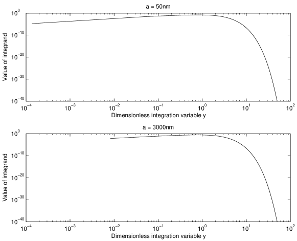
Figure 3: Same as figure 2, but with $a=\{50,3000\}$ nm, and $m=1$.

Figure 2 shows how the integrand varies with respect to $y$ for a very high Matsubara number, $m=45000$, when $a=50$ nm and $T=1$ K. The configuration is one aluminium and one copper plate. It is seen that when $y$ becomes larger than about 10, the contribution to the integral decreases rapidly. At $y=50$ the value is only $10^{-45}$. Figure 3 shows for comparison how the integrand varies with $y$ at the same temperature when the frequency is at the lowest non-vanishing value, $m=1$, for $a=50$ nm and $a=3000$ nm. The behaviour is seen to be quite similar to that above; for instance, when $y=50$ the integrand becomes approximatively $10^{-40}$. For different plate combinations, we get approximately the same behaviour. For high temperatures, the same conclusion can be drawn. In all, we found it sufficient in our computations to adopt the value

$$y_{max}=50+m\gamma$$ (13)

as general cutoff. [It is useful to note that $\gamma=2744\,(aT)$, when $a$ is given in meters and $T$ in degrees kelvin.]

Numerically, we used a method of higher order recursive adaptive quadrature. This method approximates the value of the integral with a chosen tolerance of $10^{-10}$.

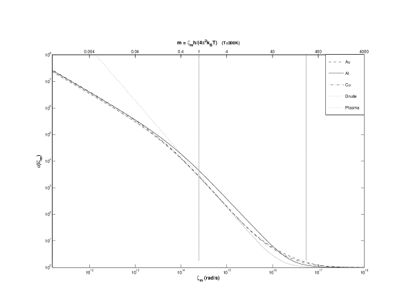
Figure 4: Numerical permittivity data for Al, Au and Cu (courtesy of Astrid Lambrecht and Serge Reynaud). Vertical lines show the frequency region that we used in the $m$ summation at $T=300$ K. Predictions from the Drude and the plasma dispersion relations are also shown in the case of Au. Top axis gives the values of the Matsubara number $m$.

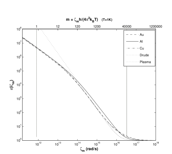
Figure 5: Same room temperature data as in figure 4, but the vertical lines show the frequency region used in the calculations at $T=1$ K. Drude and plasma dispersion relations shown for Au as before.

Next, it is useful to show the variations of $\varepsilon(i\zeta)$ graphically for the three metals mentioned, together with information about the frequency region actually used in the calculations. Figure 4 shows this for the case of $T=300$ K. The data extend over 7 decades. The vertical lines show that the important frequency region in this case lies between $2\times 10^{14}$ rad/s and $5.5\times 10^{16}$ rad/s. We also show the corresponding values of $m=\zeta_{m}\beta/2\pi$ (in nondimensional units). The range of $m$ is [1,220]. For comparison, the theoretical predictions are shown for the case of gold, both when using the Drude relation (1) and when using the plasma dispersion relation

$$\varepsilon(i\zeta)=1+\frac{\omega_{p}^{2}}{\zeta^{2}}.$$ (14)

We see that for $\zeta<1.5\times 10^{15}$ rad/s the Drude curve fits the data nicely, but for $\zeta>2\times 10^{15}$ rad/s it gives too low values for $\varepsilon$. The used frequency region corresponds to the area where the Drude prediction and the plasma prediction are approximately equal, and also to the area where the data for aluminium differ the most from the data for gold and copper.

Figure 5 shows the analogous situation when $T=1$ K. It becomes now necessary to use a much larger frequency region, from $7\times 10^{11}$ rad/s to $3.3\times 10^{16}$ rad/s, corresponding to about 80% of the entire data set. The Matsubara number region is $m\in[1,40000]$. The physical reason for this behaviour is, as always, that the case of low temperatures implies that the frequencies are very closely spaced.

3.1 Room-temperature Casimir force

We shall in this subsection assume that $T=300$ K. The force, expression (7), is always negative, but it is convenient to represent it graphically in terms of the modulus $|{\cal F}(a)|$. Since in the parallel plate-experiment of Bressi et al. [24] one was able to control the gap width down to 50 nm, we choose $a=50$ nm as our lower limit. As upper limit we choose $a=3\,\mu$m. To better visualize the results graphically, we divide all data sets into two groups, $a\in[50,200]$ nm and $a\in[200,3000]$ nm. As mentioned earlier, the plates are assumed infinite, and all roughness corrections are ignored.

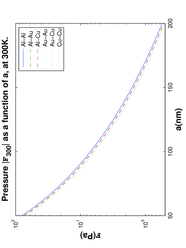
Figure 6: Casimir pressure for various combinations of metal plates, versus gap width $a\in[50,200]$ nm when $T=300$ K.

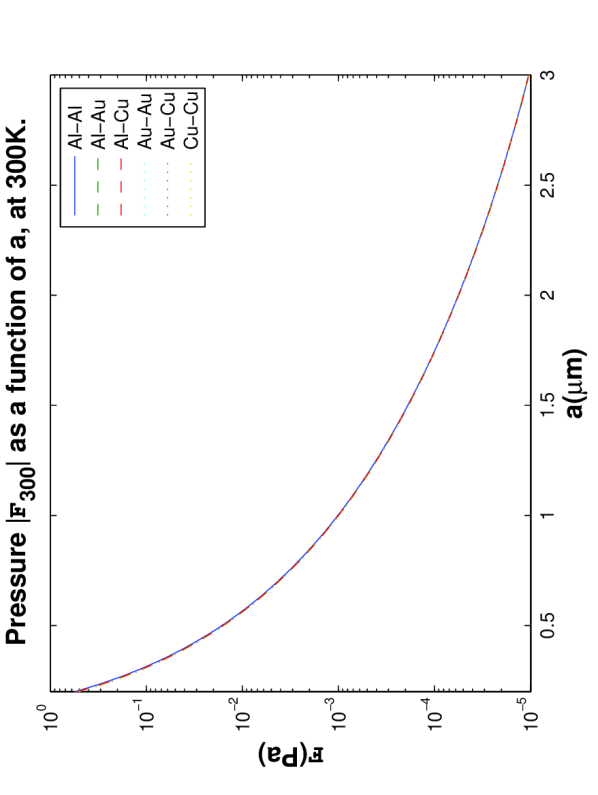
Figure 7: Same as figure 6, but with $a\in[200,3000]$ nm when $T=300$ K.

Figures 6 and 7 show how the Casimir pressure varies with $a$, for various combinations of metal plates. The force between two gold plates was computed earlier in [12], but is included here for comparison. The differences between the various combinations of the materials are seen to be small, and they diminish with increasing gap widths. The largest force always occurs for two aluminium plates. This may be called group I. The combinations aluminium-gold and aluminium-copper yield a somewhat smaller force (group II), and the last combinations Au-Au, Au-Cu and Cu-Cu result in the weakest set (group III). When $a$ increases from small to large values, the internal order in strength between the materials in groups II and III is interchanged.

3.2 Room-temperature correction, compared to $T=0$

We now turn to the finite temperature correction in the Casimir force. As mentioned above, it is then important to make clear what we mean with the zero-temperature force. Numerically, we have seen that it becomes satisfactory to represent the latter case by the choice $T=1$ K, the difference between $T=0$ and $T=1$ K being negligible.

Since the data for $\varepsilon(i\zeta)$ are measured at room temperature, the natural question becomes: can we use these data also at very low temperatures? This issue has been discussed earlier, in [11, 12, 25], with the conclusion that the temperature dependence appears not to influence the dispersion relation in a way that changes the Casimir force significantly. This implies that we can insert the same Lambrecht-Reynaud data as before, and also assume the same values for $\omega_{p}$ and $\nu$ (cf. equation (2)).

The calculated results from the $T=1$ K case are hardly distinguishable from the $T=300$ K case when plotted in the same figure. Therefore, it is better to show the calculated finite-temperature differences. In figures 8 and 9 we show the difference between the Casimir pressures at $T=1$ K and $T=300$ K,

$$\Delta{\cal F}=|{\cal F}_{1}|-|{\cal F}_{300}|,$$ (15)

versus $a$ in the range from 50 nm to 1700 nm. As the graphs for the various combinations of metals become indistinguishable for $a>0.4\,\mu$m and approach zero when $a$ becomes larger than $1.7\,\mu$m, we have omitted the region from $1.7\,\mu$m to $3\,\mu$m in figure 9.

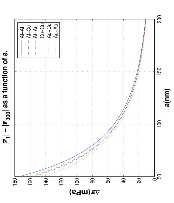
Figure 8: Difference between the Casimir pressures at $T=1$ K and $T=300$ K, equation (15), versus gap width $a$ for $a\in[50,200]$ nm.

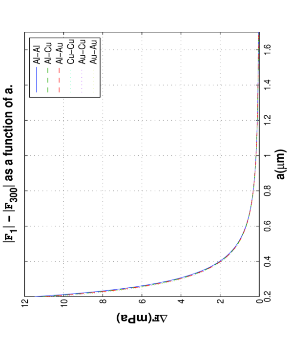
Figure 9: Same as figure 8, for the interval $a\in[200,1700]$ nm.

An important property seen from the curves is that $\Delta\cal F$ is positive. That means, the force is weaker at room temperature than at $T=0$. This is the same effect as we have pointed out earlier, in connection with identical materials in the plates [12, 10, 11]; see also [2, 23]. The behaviour is a direct consequence of the Lifshitz formula in combination with realistic permittivity data for the materials, the latter being, as we have seen, in agreement with the Drude relation at frequencies $\zeta<1.5\times 10^{15}$ rad/s. Our results for the temperature dependence are in contrast to those obtained by use of the plasma dispersion relation; in that case, the deviation of the force is positive instead of negative, and is moreover very small [14, 26, 27].

To get an overview of the magnitudes of the temperature correction, let us give some examples:

1. For small gap widths, the correction is relatively small. Thus when $a=100$ nm, the Casimir pressure is 6.105 Pa at $T=1$ K and 6.061 Pa at $T=300$ K, thus giving a room temperature reduction of 0.72%.

2. When $a=200$ nm, the respective pressures are 510 mPa at 1 K and 500 mPa at 300 K, giving a 2% reduction.

3. When $a=500$ nm, the pressures are 16.3 mPa and 15.2 mPa, giving a 6.7% reduction.

4. For large gap widths the percentage corrections become much higher, though the pressures themselves are much weaker thus making experimental work more difficult. When $a=1\,\mu$m the respective pressures are 1.12 mPa and 0.96 mPa, giving a 13.9% reduction.

It is of interest to compare the above findings with figure 5 in [10]. That figure shows, in the case of Au-Au, how the Casimir pressure varies with $aT$ when the media are assumed nondispersive. The width is assumed to be $a=1\,\mu$m. The case temperature $T=300$ K corresponds to $aT=0.131.$ One sees that in this case the agreement with our result above, ${\cal F}=0.96$ mPa, is reasonably good, if we put $\varepsilon=3000$. The broken line in figure 5 in [10] gives the result when the modified ideal metal model is used in the calculation. As already mentioned, this is an idealized model, which assumes unit reflection coefficients for all but the TE zero mode:

$$A_{0}=1,\quad B_{0}=0,\quad A_{m}=B_{m}=1\,\,{\rm for}\,\,m\geq 1.$$ (16)

The MIM model corresponds to $\varepsilon=\infty$. Putting $aT=0.131$ in the mentioned figure 5 we see that ${\cal F}\approx 1.1$ mPa. There is thus more than a 10% overprediction of the Casimir pressure following from the MIM model, at $a=1\mu$m and $T=300$ K, in comparison with our result 0.96 mPa above.

We recall again that at $T=0$ there is no distinction between a MIM model and an ”ideal metal” model (IM), for which $A_{m}=B_{m}=1$ for all $m\geq 0$. In the mentioned figure 5, setting $aT=0$, we obtain for an ideal metal ${\cal F}\approx 1.3$ mPa at $a=1\,\mu$m, which is considerably larger than the value 1.12 mPa calculated above for $T=0$.

4 A temperature correction of experimental interest

The calculated temperature correction at $T=300$ K as compared with the $T=0$ case, although of fundamental interest, will be difficult to measure in practice. For practical purposes it can thus be better to focus on temperatures that are more realistic in the laboratory. In the following, as an example, we calculate the difference between the Casimir pressures at two temperatures $T_{1}=300$ K and $T_{2}=350$ K, and let from now on $\Delta{\cal F}$ mean the pressure difference:

$$\Delta{\cal F}=|{\cal F}_{300}|-|{\cal F}_{350}|.$$ (17)

This idea of testing the Casimir force seems to go back to Chen et al. [26], and was elaborated upon also in [12].

Figures 10 and 11 show how the quantity (17) varies with $a$ in the interval $a\in[50,1400]$ nm, for the same combinations of materials as before. Again, the differences between the materials are seen to be small. Taking Au-Au as an example, we see that $\Delta{\cal F}=2.0$ mPa when $a=200$ nm. It would perhaps be possible to measure a quantity like this. The experimental advantage we see of this kind of experiment is that only force differences are involved, for a given value of the gap width. Then there will be no need of measuring the absolute Casimir pressure itself, to an extreme accuracy. (Thermal expansion effects, of course, will have to be taken into account.)

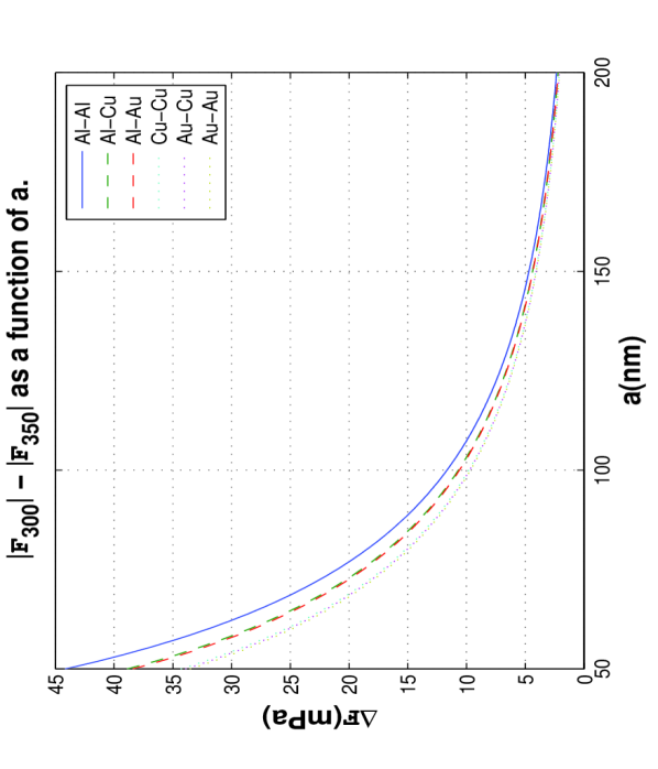
Figure 10: Difference between Casimir pressures at $T_{1}=300$ K and $T_{2}=350$ K, equation (17), versus $a$ for $a\in[50,200]$ nm.

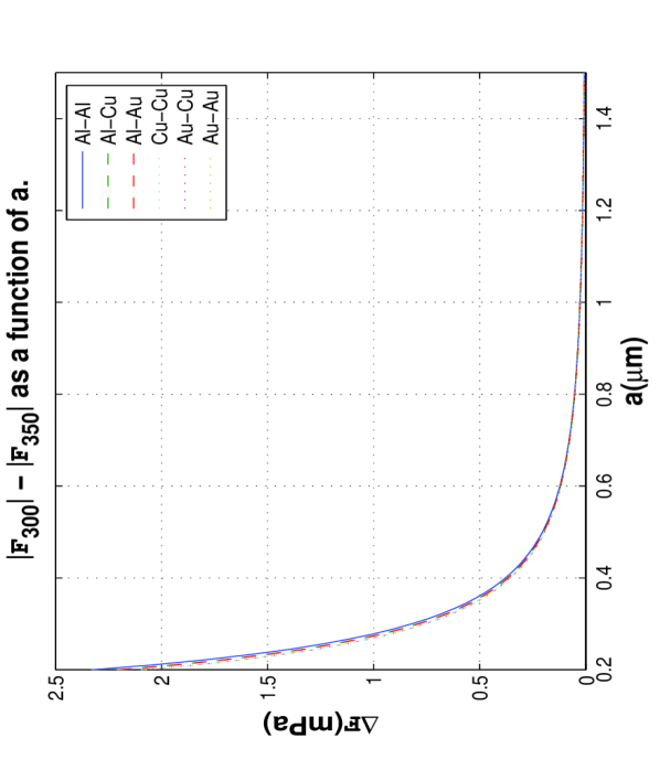
Figure 11: Same as figure 10, for the interval $a\in[200,1400]$ nm.

Finally, figure 12 shows how the relative magnitude of the difference Casimir pressure, $\Delta{\cal F}/{\cal F}_{300}$, for the same two temperatures. We see, in accordance with the behaviour above, that the relative temperature correction is greatest when $a$ is large. When $a=1.75\,\mu$m, the correction takes its maximum value, about 4%. Again, the experimental problem at large distances is that the forces themselves are so small.

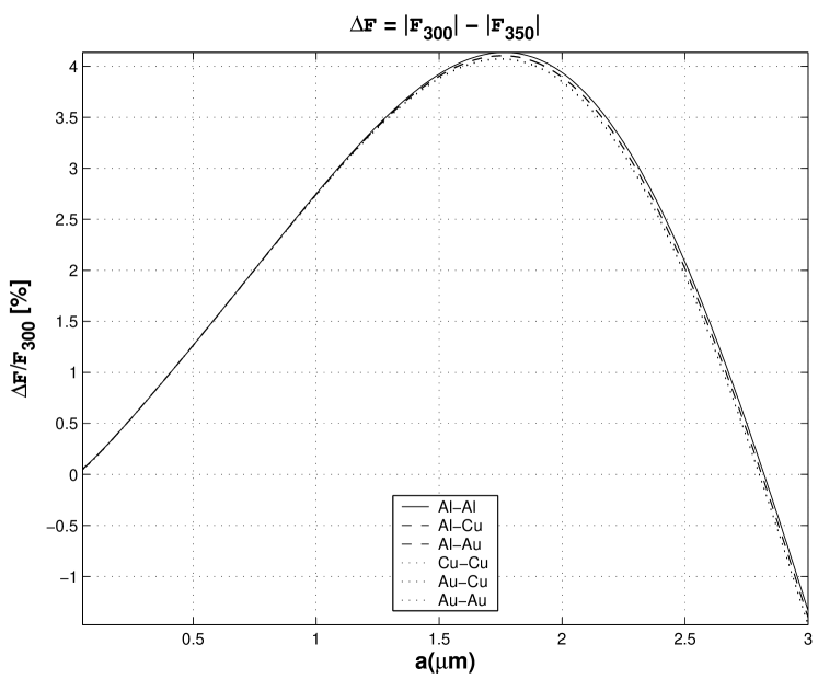
Figure 12: Relative change of the Casimir pressure, between $T_{1}=300$ K and $T_{2}=350$ K.

5 Summary

For similar and dissimilar plates, including the metals gold, copper, and aluminium, we have made accurate calculations of the Casimir pressure and have shown the results graphically. Basic elements in our calculations are the Lifshitz formula; cf. equations (3) and (7), together with realistic room-temperature values of the permittivities $\varepsilon(i\zeta)$. For frequencies $\zeta<1.5\times 10^{15}$ rad/s; cf. equations (1) and (2), the Drude dispersion relation is followed with great accuracy.

We show the results at three chosen temperatures: (i) at $T=1$ K, representing the $T=0$ case with good accuracy; (ii) at $T=300$ K; and (iii) at $T=350$ K. The low-temperature case is calculated numerically, without involving the modified ideal metal (MIM) model [10].

It turns out that the differences between the Casimir pressures for the metals investigated here are small. From figures 6 and 10, for instance, it is seen that it is the case of Al-Al surfaces that gives the strongest forces.

The most promising option for measuring the Casimir temperature correction in practice seems to be to measure the pressure difference between two practically accessible temperatures in the laboratory. As figure 12 shows, the relative change of the Casimir pressure between the temperatures 300 K and 350 K are about 4% when $a=1.75\,\mu$m. The practical problem here is that the forces themselves are so small. For lower values of $a$ the forces increase in magnitude, but the relative temperature corrections then become smaller.

Acknowledgements

We thank Astrid Lambrecht and Serge Reynaud for providing us with permittivity data for Au, Cu and Al, and we thank Jan. B. Aarseth for help with the numerics.

References

- [1] Casimir, H. B. G. 1948. Proc. Kon. Ned. Akad. Wetensch. 51, 793.
- [2] Milton, K. A. 2004. J. Phys. A: Math. Gen. 37, R209.
- [3] Milton, K. A. 2001. The Casimir Effect: Physical Manifestations of Zero-Point Energy (Singapore: World Scientific).
- [4] Bordag, M., Mohideen, U. and Mostepanenko, V. M. 2001. Phys. Rep. 353, 1.
- [5] Lamoreaux, S. K. 2005. Rep. Prog. Phys. 68, 201.
- [6] Lifshitz, E. M. 1956. Zh. Eksp. Teor. Fiz. 29, 94 [English transl.: Soviet Phys. JETP 2, 73 (1956)].
- [7] Blocki, J., Randrup, J., Swialecki, W. J. and Tsang, C. F. 1977. Ann. Phys., NY 105, 427.
- [8] Decca, R. S., López, D., Fischbach, E., Klimchitskaya, G. L., Krause, D. E. and Mostepanenko, V. M. 2005. Ann. Phys., NY 318, 37.
- [9] Brevik, I., Dahl, E. K. and Myhr, G. O. 2005. J. Phys. A: Math. Gen. 38, L49.
- [10] Høye, J. S., Brevik, I., Aarseth, J. B. and Milton, K. A. 2003. Phys. Rev. E 67, 056116.
- [11] Brevik, I., Aarseth, J. B., Høye, J. S. and Milton, K. A. 2005. Phys. Rev. E 71, 056101 (2005).
- [12] Brevik, I., Aarseth, J. B., Høye, J. S. and Milton, K. A. 2004. Proc. 6th Workshop on Quantum Field Theory Under the Influence of External Conditions, ed. K. A. Milton (Paramus, NJ: Rinton press), p. 54 [Preprint quant-ph/0311094].
- [13] Lambrecht, A. and Reynaud, S. 2000. Eur. Phys. J. D 8, 309.
- [14] Decca, R. S., Fishbach, E., Klimchitskaya, G. L., Krause, D. E., López, D. and Mostepanenko, V. M. 2003. Phys. Rev. D 68, 116003.
- [15] Boström, M. and Sernelius, Bo E. 2000. Phys. Rev. Lett. 84, 4757.
- [16] Sernelius, Bo E. and Boström, M. 2001. Phys. Rev. Lett. 87, 259101.
- [17] Boström, M. and Sernelius, Bo E. 2000. Phys. Rev. B 61, 2204.
- [18] Boström, M. and Sernelius, Bo E. 2000. Phys. Rev. B 62, 7523.
- [19] Bezerra, V. B., Decca, R. S., Fischbach, E., Geyer, B., Klimchitskaya, G. L., Krause, D. E., López, D., Mostepanenko, V. M. and Romero, C. 2005. Preprint quant-ph/0503134.
- [20] Bezerra, V. B., Klimchitskaya, G. L., Mostepanenko, V. M. and Romero, C. 2004. Phys. Rev. A 69, 022119.
- [21] Høye, J. S., Brevik, I. and Aarseth, J. B. 2001. Phys. Rev. E 63, 051101.
- [22] Brevik, I., Aarseth, J. B. and Høye, J. S. 2002. Phys. Rev. E 66, 026119.
- [23] Sernelius, Bo E. and Boström, M. 2004. Proc. 6th Workshop on Quantum Field Theory Under the Influence of External Conditions, ed. K. A. Milton (Paramus, NJ: Rinton press), p. 82.
- [24] Bressi, G., Carugno, G., Onofrio, R. and Ruoso, G. 2002. Phys. Rev. Lett. 88, 041804.
- [25] Boström, M. and Sernelius, B. E. 2004. Physica A 339, 53.
- [26] Chen, F., Klimchitskaya, G. L., Mohideen, U. and Mostepanenko, V. M. 2003. Phys. Rev. Lett. 90, 160404.
- [27] Chen, F., Klimchitskaya, G. L., Mohideen, U. and Mostepanenko, V. M. 2004. Phys. Rev. A 69, 022117.