Quantum phase-space description of light polarization

Abstract

We present a method to characterize the polarization state of a light field in the continuous-variable regime. Instead of using the abstract formalism of SU(2) quasidistributions, we model polarization in the classical spirit by superposing two harmonic oscillators of the same angular frequency along two orthogonal axes. By describing each oscillator by a $s$-parametrized quasidistribution, we derive in a consistent way the final function for the polarization. We compare with previous approaches and discuss how this formalism works in some relevant examples.

1 Introduction

Polarization is a fundamental property of light, both in the quantum and in the classical domain. In quantum optics, polarization has been mainly examined in the single-photon regime [1, 2, 3, 4, 5, 6, 7]. Nevertheless, different schemes have been proposed [8, 9] and experimentally implemented [10, 11] to characterize the continuous-variable limit of the quantum Stokes parameters. We stress that these continuous-variable polarization states can be carried by a bright laser beam providing high bandwidth capabilities and therefore faster signal transfer rates than single photon systems. In addition, they retain the single-photon advantage of not requiring the universal local oscillator necessary for other proposed continuous variable quantum networks.

Since the seminal paper of Wigner [12], and the major contributions of Moyal [13], Stratonovich [14], and Berezin [15], it seems indisputable that phase-space methods, based on using quasidistributions that reflect the noncommutatibility of quantum observables, constitute a valuable tool in examining continuous variables in quantum optics [16, 17, 18].

In particular, these methods have had great success in analyzing one-mode fields; i. e., Heisenberg-Weyl quasidistributions representing the quantum dynamics in the flat $q$-$p$ (or, equivalently, $a$-$a^{\ast}$) space. Although not so popular in the quantum-optics community, spinlike systems, with the sphere $\mathcal{S}_{2}$ as phase space, have been also discussed at length in this framework [19, 20, 21, 22, 23, 24, 25, 26, 27]. The resulting functions, naturally related to the SU(2) dynamical group, have been used to visualize, e. g., nonclassical properties of a collection of two-level atoms [28].

Since the Stokes operators can be formally identified with an angular momentum [29, 30, 31, 32], one may naively expect a direct translation of these SU(2) quasidistributions to the problem of polarization. However, this is not the case, mainly because they act on different types of Hilbert space [33]. We can then conclude that the problem of an adequate quasiclassical description of polarization of light is still an open question [34, 35].

The Stokes operators are a particular case of the Schwinger map [36], with two kinematically independent oscillators. In this spirit, it has been recently shown that the Stokes operators are the constants of motion of the two-dimensional isotropic harmonic oscillator [37]. This reflects the fact that the polarization of a classical field can be adequately viewed as the Lissajous figure traced out by the end of the electric vector of a monochromatic field [38]. In sharp contrast, in quantum optics the probability distribution for the electric field can be very far from having an elliptical form [39, 40].

We wish to investigate this point from the perspective of quasidistributions. We show that one can start from the $s$-ordered quasidistributions from two kinematically independent oscillators: by eliminating an unessential common phase, we get well-behaved quasidistributions on the Poincaré sphere. We apply the resulting family of polarization quasidistributions to some relevant states, and conclude that they constitute an appropriate tool to deal with such a basic variable.

2 Phase-space representation of a harmonic oscillator

To keep the discussion as self-contained as possible, we first briefly summarize the essential ingredients of phase-space functions for a harmonic oscillator that we shall need for our purposes.

In the Hilbert space $\mathcal{H}$, the state of the system is fully represented by its density operator $\hat{\varrho}$. In the phase-space formalism, $\hat{\varrho}$ is mapped by a family of functions (quasidistributions) $W^{(s)}(\alpha)$ onto the classical phase space $X$ ($\alpha\in X$). This map is usually implemented by the generalized Weyl rule [26]

$$W^{(s)}(\alpha)=\mathop{\mathrm{Tr}}\nolimits[\hat{\varrho}\,\hat{w}^{(s)}(\alpha)],$$ (1)

where the generating kernel $\hat{w}^{(s)}(\alpha)$ fulfill the general properties

$$\begin{array}[]{l}\hat{w}^{(s)}(\alpha)=[\hat{w}^{(s)}(\alpha)]^{\dagger},\\ \\ \displaystyle\int_{X}d\mu(\alpha)\,\hat{w}^{(s)}(\alpha)=\hat{\leavevmode\hbox{\small 1\normalsize\kern-3.30002pt1}}.\end{array}$$ (2)

The index $s$ that labels functions in the family is related to the $s$ ordering. The values $-1$, $+1$, and $0$ correspond to the normal, antinormal, and symmetric ordering, respectively, or equivalently to the $P$, $Q$, and $W$ functions. We stress that these quasidistributions can be determined in practice by using simple and efficient experimental procedures [41, 42, 43, 44, 45, 46]. Moreover, they provide a simple measure of the nonclassical behavior of quantum states [47, 48, 49, 50].

Let us now turn to the outstanding case of a harmonic oscillator represented by annihilation and creation operators $\hat{a}$ and $\hat{a}^{\dagger}$, that obey the canonical commutation relation

$$[\hat{a},\hat{a}^{\dagger}]=\hat{\leavevmode\hbox{\small 1\normalsize\kern-3.30002pt1}}.$$ (3)

The phase space is the complex plane $\mathbb{C}$ and the invariant measure is $d\mu(\alpha)=d^{2}\alpha/\pi^{2}$. The operator

$$\hat{D}(\alpha)=\exp(\alpha\hat{a}^{\dagger}-\alpha^{\ast}\hat{a})$$ (4)

is the standard displacement operator in the complex plane $\alpha$ and leads to introduce the standard coherent states as

$$|\alpha\rangle=\hat{D}(\alpha)|0\rangle,$$ (5)

where $|0\rangle$ denotes the ground state. In this case, the kernel $\hat{w}^{(s)}(\alpha)$ is exactly the Cahill-Glauber kernel

$$\hat{w}^{(s)}(\alpha)=\frac{1}{\pi^{2}}\int_{\mathbb{C}}d^{2}\beta\,e^{-s|\beta|^{2}/2}\,\exp(\alpha\beta^{\ast}-\alpha^{\ast}\beta)\,\hat{D}(\alpha).$$ (6)

It is often useful to represent this operator in a somewhat different form. After some calculations, it turns out that (6) may be rewritten as [50]

$$\hat{w}^{(s)}(\alpha)=\frac{2}{1-s}\hat{D}(\alpha)\ \left(\frac{s+1}{s-1}\right)^{\hat{a}^{\dagger}\hat{a}}\ \hat{D}^{\dagger}(\alpha),$$ (7)

which can also be represented in a disentangled form

$$\hat{w}^{(s)}(\alpha)=\frac{2}{1-s}\,e^{-\frac{2|\alpha|^{2}}{1-s}}\left(\frac{s+1}{s-1}\right)^{\hat{a}^{\dagger}\hat{a}}\exp\left(-\frac{2\alpha}{1+s}\hat{a}^{\dagger}\right)\exp\left(\frac{2\alpha^{\ast}}{1-s}\hat{a}\right).$$ (8)

The reader is referred to e.g. Ref. [17] to see how this $s$-parametrized representation works for some elementary field states.

3 Phase-space description of two orthogonal harmonic oscillators

In classical optics, the superposition of two oscillations of the same angular frequency $\omega$, one along the horizontal axis $H$ and the other along the vertical axis $V$, results in an elliptical motion. This is the simplest Lissajous figure and is the basic physics behind the notion of light polarization.

To translate this picture into quantum optics, we assume that the two oscillators are represented by the complex amplitude operators $\hat{a}_{H}$ ($\hat{a}_{H}^{\dagger}$) and $\hat{a}_{V}$ ($\hat{a}_{V}^{\dagger}$), fulfilling (3); i. e.,

$$[\hat{a}_{j},\hat{a}_{k}^{\dagger}]=\delta_{jk}\hat{\leavevmode\hbox{\small 1\normalsize\kern-3.30002pt1}}\,,\qquad\qquad j,k=H,V.$$ (9)

In phase space, these oscillators can be appropriately described by the product of the corresponding kernel operators

$$\hat{w}^{(s)}(\alpha_{H},\alpha_{V})=\hat{w}^{(s)}(\alpha_{H})\,\hat{w}^{(s)}(\alpha_{V}).$$ (10)

A Lissajous figure needs only three independent quantities to be fully characterized: the amplitudes of each oscillator and the relative phase between them. We therefore introduce the parametrization

$$\alpha_{H}=re^{i\zeta}\cos(\theta/2),\qquad\alpha_{V}=re^{i\zeta}e^{-i\phi}\sin(\theta/2),$$ (11)

where

$$r^{2}=|\alpha_{H}|^{2}+|\alpha_{V}|^{2}$$ (12)

is a radial variable related with the global intensity. The parameters $\theta$ and $\phi$ can be interpreted as the polar and azimuthal angles, respectively, on the Poincaré sphere $\mathcal{S}_{2}$. In terms of this parametrization, equation (10) can be recast as

$$\hat{w}^{(s)}(\alpha_{H},\alpha_{V}) = \left(\frac{2}{1-s}\right)^{2}e^{-\frac{2r^{2}}{1-s}}\left(\frac{s+1}{s-1}\right)^{\hat{N}}$$

$$\times \hat{U}(\theta,\phi)\,\left[\exp\left(-\frac{2r}{1+s}e^{i\zeta}\hat{a}_{H}^{\dagger}\right)\exp\left(\frac{2r}{1-s}e^{-i\zeta}\hat{a}_{H}\right)\right]\,\hat{U}^{\dagger}(\theta,\phi),$$

where

$$\hat{N}=\hat{a}_{H}^{\dagger}\hat{a}_{H}+\hat{a}_{V}^{\dagger}\hat{a}_{V}$$ (14)

is the operator representing the total number of excitations and

$$\hat{U}(\theta,\phi)=\exp\left[\frac{\theta}{2}\left(e^{-i\phi}\hat{a}_{H}\hat{a}_{V}^{\dagger}-e^{i\phi}\hat{a}_{V}\hat{a}_{H}^{\dagger}\right)\right].$$ (15)

We next proceed to integrate over the physically irrelevant global phase $\zeta$:

$$\hat{w}^{(s)}(r,\theta,\phi) = \frac{1}{2\pi}\int_{-\pi}^{\pi}d\zeta\ \hat{w}^{(s)}(\alpha_{H},\alpha_{V})=\left(\frac{2}{1-s}\right)^{2}e^{\frac{2r^{2}}{1-s}}\left(\frac{s+1}{s-1}\right)^{\hat{N}}$$ (16)

$$\times \hat{U}(\theta,\phi)\ \left[\sum_{\ell=0}^{\infty}\frac{(-1)^{\ell}}{\ell!^{2}}r^{2\ell}\left(\frac{4}{1-s^{2}}\right)^{\ell}\hat{a}_{H}^{\dagger\ell}\hat{a}_{H}^{\ell}\right]\ \hat{U}^{\dagger}(\theta,\phi)\,.$$

Finally, we integrate over the radial variable $r$ (with the weight $2r^{2}$) to obtain the phase-space kernel over the sphere $\mathcal{S}_{2}$

$$\hat{w}^{(s)}(\theta,\phi) = 2\int_{0}^{\infty}dr\ r^{3}\,\hat{w}^{(s)}(\theta,\phi,r)=\left(\frac{s+1}{s-1}\right)^{\hat{N}}$$ (17)

$$\times \hat{U}(\theta,\phi)\ \left[\sum_{\ell=0}^{\infty}(-1)^{\ell}\,\frac{\ell+1}{\ell!}\left(\frac{2}{1+s}\right)^{\ell}\hat{a}_{H}^{\dagger\ell}\hat{a}_{H}^{\ell}\right]\ \hat{U}^{\dagger}(\theta,\phi)\,.$$

If we observe that

$$\sum_{\ell=0}^{\infty}\frac{z^{\ell}}{\ell!}\;\hat{a}_{H}^{\dagger\ell}\hat{a}_{H}^{\ell}=(z+1)^{\hat{a}_{H}^{\dagger}\hat{a}_{H}}\,,$$ (18)

we easily obtain

$$\hat{w}^{(s)}(\theta,\phi) = \left(\frac{s+1}{s-1}\right)^{\hat{N}}\ \hat{U}(\theta,\phi)\ \left[\left(\frac{s-1}{s+1}\right)^{\hat{a}_{H}^{\dagger}\hat{a}_{H}}\frac{2\hat{a}_{H}^{\dagger}\hat{a}_{H}+1-s}{1-s}\right]\ \hat{U}^{\dagger}(\theta,\phi)$$ (19)

$$= \hat{U}(\theta,\phi)\ \left[\left(\frac{s+1}{s-1}\right)^{\hat{a}_{V}^{\dagger}\hat{a}_{V}}\frac{2\hat{a}_{H}^{\dagger}\hat{a}_{H}+1-s}{1-s}\right]\ \hat{U}^{\dagger}(\theta,\phi)\,.$$

This is our central and compact result, that we shall work out in detail in the rest of the paper.

For the antisymmetric ordering $(s=-1)$, which corresponds to the $Q$-function, (19) reduces to

$$\hat{w}^{(-1)}(\theta,\phi)=\hat{U}(\theta,\phi)\ \left[\lim_{s\rightarrow-1}\left(\frac{s+1}{s-1}\right)^{\hat{a}_{V}^{\dagger}\hat{a}_{V}}(\hat{a}_{H}^{\dagger}\hat{a}_{H}+1)\right]\ \hat{U}^{\dagger}(\theta,\phi)\,.$$ (20)

To proceed further we notice that

$$\lim_{s\rightarrow-1}\left(\frac{s+1}{s-1}\right)^{\hat{a}_{V}^{\dagger}\hat{a}_{V}}=\sum_{N=0}^{\infty}|N,0\rangle\ \langle N,0|$$ (21)

is precisely the projector on the subspace with zero excitations in the vertical mode $V$. Henceforth, we shall denote by

$$|N,k\rangle:=|N-k\rangle_{H}\otimes|k\rangle_{V}$$ (22)

a state with $N-k$ excitations in the horizontal mode $H$ and $k$ in the vertical mode $V$. In view of (21) we have

$$\hat{w}^{(-1)}(\theta,\phi)=\sum_{N=0}^{\infty}(N+1)|N,\theta,\phi\rangle\langle N,\theta,\phi|\,,$$ (23)

where $|N,\theta,\phi\rangle$ are the standard SU(2) coherent states [51]

$$|N,\theta,\phi\rangle = \hat{U}(\theta,\phi)|N,0\rangle$$ (26)

$$= \sum_{k=0}^{N}\left(\begin{array}[]{c}N\\ k\end{array}\right)^{1/2}\left(\sin\frac{\theta}{2}\right)^{k}\left(\cos\frac{\theta}{2}\right)^{N-k}\ e^{-ik\phi}|N,k\rangle\,.$$

The $Q$ function generated by this kernel reads as

$$Q(\theta,\phi)=\mathop{\mathrm{Tr}}\nolimits[\hat{\varrho}\hat{w}^{(-1)}(\theta,\phi)]=\sum_{N=0}^{\infty}(N+1)\ Q(N,\theta,\phi)\,,$$ (27)

where

$$Q(N,\theta,\phi)=\langle N,\theta,\phi|\hat{\varrho}|N,\theta,\phi\rangle\,.$$ (28)

The normalization condition

$$\frac{1}{4\pi}\int d\Omega\ Q(\theta,\phi)=1\,,$$ (29)

where $d\Omega=\sin\theta d\theta d\phi$ is the differential of solid angle, is automatically fulfilled.

Equation (27) is a well-known result, which may be derived from a variety of methods. The point we wish to stress is here that (27) involves only diagonal elements between states with the same number of excitations. Because of the lack of the off-diagonal contributions of the form $\langle N,\theta,\phi|\hat{\varrho}|N^{\prime},\theta,\phi\rangle$ with $N\neq N^{\prime}$, the $Q$ function takes the form of an average over the subspaces with definite total number of excitations. The role of the sum in $N$ is to remove the total intensity from the description of the state.

We next pass to the symmetrical order ($s=0$), which corresponds to the Wigner function. From (19) we immediately get

$$\hat{w}^{(0)}(\theta,\phi)=\hat{U}(\theta,\phi)\ \left[(-1)^{\hat{a}_{V}^{\dagger}\hat{a}_{V}}(2\hat{a}_{H}^{\dagger}\hat{a}_{H}+1)\right]\ \hat{U}^{\dagger}(\theta,\phi).$$ (30)

To properly transform the operator in brackets, it proves convenient to introduce the following operators

$$\hat{J}_{x} = \frac{1}{2}(\hat{a}_{H}^{\dagger}\hat{a}_{V}+\hat{a}_{V}^{\dagger}\hat{a}_{H})\,,$$

$$\hat{J}_{y} = \frac{1}{2i}(\hat{a}_{H}^{\dagger}\hat{a}_{V}-\hat{a}_{V}^{\dagger}\hat{a}_{H})\,,$$ (31)

$$\hat{J}_{z} = \frac{1}{2}(\hat{a}_{H}^{\dagger}\hat{a}_{H}-\hat{a}_{V}^{\dagger}\hat{a}_{V})\,,$$

which constitute the Schwinger map for two independent oscillators [36] and are the generators of the group SU(2). Since $\hat{U}(\theta,\phi)$ is an element of SU(2), it can be represented as [51]

$$\hat{U}(\theta,\phi)=e^{-i\phi\hat{J}_{z}}\ e^{-i\theta\hat{J}_{y}}\ e^{i\phi\hat{J}_{z}}.$$ (32)

Next, we note that $\hat{a}_{H}^{\dagger}\hat{a}_{H}=\hat{N}/2-\hat{J}_{z}$ and that

$$\hat{U}(\theta,\phi)\ \hat{J}_{z}\ \hat{U}^{\dagger}(\theta,\phi)=\hat{\mathbf{J}}\cdot\mathbf{n}\,,$$ (33)

where $\hat{\mathbf{J}}=(\hat{J}_{x},\hat{J}_{y},\hat{J}_{z})$ and $\mathbf{n}=(\sin\theta\cos\phi,\sin\theta\sin\phi,\cos\theta)$ is a unit vector on the sphere $\mathcal{S}_{2}$. Then, equation (30) simplifies to

$$\hat{w}^{(0)}(\theta,\phi)=(-1)^{\hat{N}/2}(\hat{N}-2\hat{\mathbf{J}}\cdot\mathbf{n}+\hat{\leavevmode\hbox{\small 1\normalsize\kern-3.30002pt1}})\ \hat{U}(\theta,\phi)\ \exp(-i\pi\hat{J}_{z})\ \hat{U}^{\dagger}(\theta,\phi).$$ (34)

This Wigner function will be examined for a variety of states in the next section. However, it seems pertinent to compare before these results with previous approaches using the machinery of SU(2) quasidistributions. One can immediately check that both give the same $Q$ function, meanwhile the corresponding Wigner functions are different. Once again, the symmetrical order is extraordinarily sensitive to any fingerprint of nonclassical behavior. Without going into mathematical details, we merely quote that, as shown in Ref. [52], the SU(2) Wigner kernel can be represented as

$$\hat{w}_{\mathrm{SU(2)}}^{(0)}(\theta,\phi)=\hat{U}(\theta,\phi)\ F(\hat{J}_{z})\ \hat{U}^{\dagger}(\theta,\phi),$$ (35)

where $F(\hat{J}_{z})$ is an operator whose expression is of little interest for our purposes here. It turns out, however, that in the asymptotic case of large dimensions of the representation ($J\gg 1$), $F(\hat{J}_{z})$ tends to the parity operator on the sphere: $F(\hat{J}_{z})\rightarrow\ \exp(-i\pi\hat{J}_{z})$. The SU(2) Wigner function coincides thus with (34), except for the factor the appears premultiplying, which does not play any relevant role. So, in the classical limit, both approaches give the same result. Nevertheless, we mention that the SU(2) quasidistributions have been not determined experimentally yet, at difference of the easy measurability of the $s$-ordered quasidistributions for the single polarization modes.

We finally note that the operator (34), when restricted to a single SU(2) invariant subspace, does not contain complete information: in other words, it cannot be inverted to obtain the density matrix.

4 Examples and concluding remarks

To gain further insights into this formalism, we shall particularize the Wigner function (34) for several states of interest. For simplicity, we assume a pure state $|\Psi\rangle$, so that the Wigner function is simply

$$W(\theta,\phi)=\mathop{\mathrm{Tr}}\nolimits[\hat{\varrho}(\theta,\phi)\ (-1)^{\hat{a}_{V}^{\dagger}\hat{a}_{V}}(2\hat{a}_{H}^{\dagger}\hat{a}_{H}+\hat{\leavevmode\hbox{\small 1\normalsize\kern-3.30002pt1}})],$$ (36)

where

$$\hat{\varrho}(\theta,\phi)=\hat{U}^{\dagger}(\theta,\phi)\ |\Psi\rangle\langle\Psi|\ \hat{U}(\theta,\phi).$$ (37)

We recall that, for fixed $N$, the states $|N,k\rangle$ $(k=0,\ldots,N$) span a $(N+1)$-dimensional invariant subspace, wherein the action of the operators (3) is standard. In consequence, we expand $|\Psi\rangle$ in this basis

$$|\Psi\rangle=\sum_{N=0}^{\infty}\sum_{k=0}^{N}\Psi_{Nk}|N,k\rangle,$$ (38)

so that the action of $\hat{U}(\theta,\phi)$ on $|\Psi\rangle$ can be easily calculated. The resulting Wigner function takes the form

$$W(\theta,\phi) = \sum_{N=0}^{\infty}\sum_{k,m,n=0}^{N}(-1)^{n}\,(2N-2n+1)$$ (39)

$$\times \Psi_{Nk}\Psi_{Nm}^{\ast}\,e^{i\phi(k-m)}\,d_{nk}^{N}(-\theta)d_{mn}^{N}(\theta),$$

where $d_{nk}^{N}(\theta)$ is the Wigner $d$ function

$$d_{k^{\prime}k}^{N}(\theta)=\langle N,k^{\prime}|\exp(i\theta\hat{J}_{y})|N,k\rangle,$$ (40)

whose properties have been extensively studied [53]. Using such properties and after some lengthy, but otherwise straightforward calculations, we finally get

$$W(\theta,\phi) = \sum_{N=0}^{\infty}\sum_{m,n=0}^{N}(-1)^{n}[N+1+(m+n-N)/\cos\theta]$$ (41)

$$\times \Psi_{Nm}\Psi_{Nn}^{\ast}\,e^{i\phi(m-n)}\,d_{nm}^{N}(-2\theta).$$

It can be checked that $W(\theta,\phi)$ is properly normalized

$$\frac{1}{4\pi}\int d\Omega\ W(\theta,\phi)=1.$$ (42)

We first consider the case of (quadrature) coherent states

$$|\Psi\rangle=|\alpha_{H}\rangle_{H}\otimes|\alpha_{V}\rangle_{V}.$$ (43)

We take both oscillators with the same amplitude and relative phase $\varphi$; i.e., $\alpha_{H}=r/\sqrt{2}$ and $\alpha_{V}=r/\sqrt{2}e^{-i\varphi}$. This is perhaps the most interesting situation as polarization is concerned. The decomposition in invariant subspaces reads

$$\Psi_{Nk}=e^{-|\alpha|^{2}}\frac{|\alpha|^{N}}{\sqrt{(N-k)!k!}}e^{ik\varphi},$$ (44)

Note that this state is separable and $\Psi_{Nk}$ is just the product of the photon-number amplitudes in each polarization mode. The sums in (41) can be carried out explicitly, with the result

$$W(\theta,\phi)=\left\{r^{2}[1+\sin\theta\cos(\phi+\varphi)]+1\right\}\exp\left\{-2r^{2}[1-\sin\theta\cos(\phi+\varphi)]\right\}.$$

To examine how the quantum character of the state reflects itself in the properties of the Wigner function, we plot the distribution [28]

$$f(\theta,\phi)=1+\frac{W(\theta,\phi)}{\langle\hat{N}\rangle}$$ (46)

on the unit sphere. Notice that, with our parametrization, if the unit vector $\mathbf{n}$ points in the positive direction $x$, $y$, or $z$ the state is right-circularly, linearly at 45^∘, or horizontally polarized light, respectively. In Fig. 1 we have plotted the normalized probability distribution $f(\theta,\phi)$ for the coherent case, with $r=5$ and the relative phase $\varphi=\pi/2$, which classically corresponds to circularly polarized light. What we see in the figure is indeed a Gaussian distribution centered at the corresponding classical point.

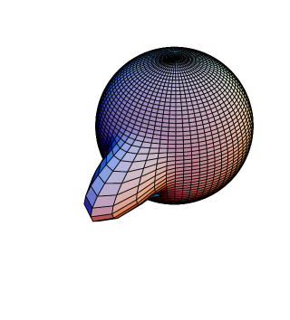
Figure 1: Spherical plot of the normalized distribution (46) when the two polarization modes are in a coherent state. We take both amplitudes equal to $r=5$ and the relative phase $\varphi=\pi/2$. The Gaussian is centered at the classical point corresponding to right-circularly polarized light.

Next we consider coherent squeezed states in both polarization modes. In consequence, we have

$$|\Psi\rangle=|\alpha_{H},\xi_{H}\rangle_{H}\otimes|\alpha_{V},\xi_{V}\rangle_{V}\,,$$ (47)

where

$$|\alpha,\xi\rangle=\hat{S}(\xi)|\alpha\rangle.$$ (48)

Here $|\alpha\rangle$ denotes a coherent state and

$$\hat{S}(\xi)=\exp\left[-\frac{1}{2}(\xi^{\ast}\hat{a}^{2}-\xi\hat{a}^{\dagger 2})\right]$$ (49)

is the squeeze operator. The complex number $\xi$ is known as the squeezing parameter and is usually expressed $\xi=|\xi|e^{i\vartheta}$: while $|\xi|$ measures the squeezing of the fluctuations, $\vartheta$ measures the direction in which such a squeezing takes place.

The state is again separable and the decomposition (38) is now

$$\Psi_{Nk}={}_{H}\langle N-k|\alpha_{H},\xi_{H}\rangle_{H}\;{}_{V}\langle k|\alpha_{V},\xi_{V}\rangle_{V}.$$ (50)

The photon-number amplitude for each polarization mode is

$$\langle k|\alpha,\xi\rangle=\frac{[\nu/(2\mu)]^{k/2}}{\sqrt{\mu\,k!}}\exp\left[-\frac{1}{2}\left(|\alpha|^{2}-\frac{\nu^{\ast}}{\mu}\alpha^{2}\right)\right]\mathrm{H}_{k}\left(\frac{\alpha}{\sqrt{2\mu\nu}}\right),$$ (51)

where $\mathrm{H}_{k}(x)$ are the Hermite polynomials and we have used the notation

$$\mu=\cosh|\xi|,\qquad\qquad\nu=e^{i\vartheta}\sinh|\xi|.$$ (52)

In this case, we have found no simple closed expression for the Wigner function (41). Nevertheless, numerical calculations are simple. In Fig. 2 we have represented the normalized distribution (46) when both modes are in the same squeezed state with a real coherent amplitude $\alpha=5$ and a squeezing factor $|\xi|=0.3$ in the direction $\vartheta=0$. Apart from a small deformation of the sphere, we see two symmetrical peaks with elliptical contours that indeed represent squeezing of the fluctuations.

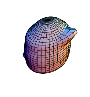
Figure 2: Spherical plot of the normalized distribution (46) when the two polarization modes are in a squeezed state. We take both modes in the same state, with a coherent amplitude $\alpha=5$ and a squeezing factor $|\xi|=0.3$ in the direction $\vartheta=0$.

To give another simple but illustrative example, we consider a two-mode squeezed vacuum state

$$|\Psi\rangle=\hat{S}(\xi)(|0\rangle_{H}\otimes|0\rangle_{V}),$$ (53)

where the two-mode squeeze operator is

$$\hat{S}(\xi)=\exp\left(\xi^{\ast}\hat{a}_{H}\hat{a}_{V}-\xi\hat{a}_{V}^{\dagger}\hat{a}_{H}^{\dagger}\right)\,,$$ (54)

and $\mu$ and $\nu$ are defined as in equation (52). The decomposition in invariant subspaces for this state is

$$\Psi_{Nk}=\delta_{N,2k}\frac{1}{\mu}\left(-\frac{\nu}{\mu}\right)^{k}.$$ (55)

The Wigner function (41) can be expressed again in a closed form:

$$W(\theta,\phi)=\frac{1}{|\mu|^{2}}\frac{1-|\nu/\mu|^{2}}{[1+2|\nu/\mu|\cos(2\theta)+|\nu/\mu|^{2}]^{3/2}}.$$ (56)

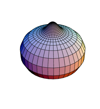
Figure 3: Spherical plot of the normalized distribution (46) for a two-mode squeezed vacuum state with a squeezing parameter $|\xi|=0.9$.

In Fig. 3 we have plotted the normalized distribution corresponding to a two-mode squeezed vacuum with $|\xi|=0.9$. We see the presence of two Gaussian cups centered at the north and south poles and also a belt around the equator of the unit sphere. This state can be seen as arising mainly from these contributions and is rotationally symmetric, as (56) is independent of $\phi$.

Finally, we consider the propagation of light in a Kerr medium. If initially both polarization modes are in coherent states of amplitudes $\alpha_{H}$ and $\alpha_{V}$, the state at time $t$ can be written as [54, 55, 56, 57, 58]

$$|\Psi(\tau)\rangle=\hat{T}(\tau)(|\alpha_{H}\rangle_{H}\otimes|\alpha_{V}\rangle_{V}),$$ (57)

where

$$\hat{T}(\tau)=\exp\left(i\tau\hat{a}_{H}^{\dagger}\hat{a}_{H}\ \hat{a}_{V}^{\dagger}\hat{a}_{V}\right),$$ (58)

and $\tau=\chi t$, $\chi$ being a real parameter proportional to the third-order nonlinear susceptibility of the medium. The state (57) is entangled, and its expansion (38) can be easily worked out

$$\Psi_{Nk}=e^{i\tau(N-k)k}\ e^{-(|\alpha_{H}|^{2}+|\alpha_{V}|^{2})}\ \frac{|\alpha_{H}|^{N-k}|\alpha_{V}|^{k}}{\sqrt{(N-k)!k!}}.$$ (59)

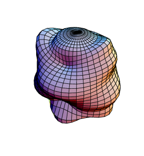
Figure 4: Spherical plot of the normalized distribution (46) for light propagating in a Kerr medium. Initially the state is coherent in both polarization modes with amplitude $r=5$ and the (adimensional) propagation time is $\tau=\pi/2$.

The presence of the quadratic phase in (59) prevents again from obtaining an analytical form for the Wigner function. In Fig. 4 we show the normalized distribution on the sphere for a coherent amplitude $r=5$ equal in both polarization modes and $\tau=\pi/2$. The complicated phase dynamics predicted by the theory manifests itself in a complex pattern of well resolved peaks.

In summary, what we expect to have accomplished in this paper is to present a simple alternative phase-space formalism for polarization on the Poincaré sphere, based on $s$-ordered quasidistributions for the two basic polarization modes. These results may have interesting experimental consequences in order to implement a feasible experimental procedure for determining polarization properties.

References

• [1] A. Peres, Quantum Theory: Concepts and Methods, Kluwer, Dordrecht, 1993.
• [2] P. G. Kwiat, K. Mattle, H. Weinfurter, A. Zeilinger, A. V. Sergienko, Y. Shih, Phys. Rev. Lett. 75 (1995) 4337.
• [3] K. Mattle, H. Weinfurter, P. G. Kwiat, A. Zeilinger, Phys. Rev. Lett. 76 (1996) 4656.
• [4] A. Muller, T. Hertzog, B. Huttner, W. Tittel, H. Zbinden, N. Gisin, Appl. Phys. Lett. 70 (1997) 793.
• [5] A. Zeilinger, Rev. Mod. Phys. 71 (1999) S288.
• [6] A. Trifonov, G. Björk, J. Söderholm, Phys. Rev. Lett. 86 (2001) 4423.
• [7] M. Barbieri, F. De Martini, G. Di Nepi, P. Mataloni, G. M. D’Ariano, C. Macchiavello, Phys. Rev. Lett. 91 (2003) 227901.
• [8] A. P. Alodjants, S. M. Arakelian, A. S. Chirkin, Appl. Phys. B 66 (1998) 53.
• [9] N. V. Korolkova, G. Leuchs, R. Loudon, T. C. Ralph, C. Silberhorn, Phys. Rev. A 65 (2002) 052306.
• [10] P. Grangier, R. E. Slusher, B. Yurke, A. LaPorta, Phys. Rev. Lett. 59 (1987) 2153.
• [11] W. P. Bowen, R. Schnabel, H.-A. Bachor, P. K. Lam, Phys. Rev. Lett. 88 (2002) 093601.
• [12] E. P. Wigner, Phys. Rev. 40 (1932) 749.
• [13] J. E. Moyal, Proc. Camb. Phil. Soc. 45 (1949) 99.
• [14] R. L. Stratonovich, Sov. Phys. JETP 31 (1956) 1012.
• [15] F. A. Berezin, Commun. Math. Phys. 40 (1975) 153.
• [16] M. Hillery, R. F. O’ Connell, M. O. Scully, E. P. Wigner, Phys. Rep. 106 (1984) 121.
• [17] V. Peřinová, A. Lukš, J. Peřina, Phase in Optics, World Scientific, Singapore, 1998.
• [18] W. P. Schleich, Quantum Optics in Phase Space Wiley-VCH, Weinheim, 2001.
• [19] G. S. Agarwal, Phys. Rev. A 24 (1981) 2889.
• [20] L. Cohen, M. O. Scully, Found. Phys. 16 (1986) 295
• [21] J. C. Várilly, J. M. Gracia-Bondía, Ann. Phys. (N. Y.) 190 (1989) 107.
• [22] K. B. Wolf, Opt. Commun. 132 (1996) 343.
• [23] G. Ramachandran, A. R. Usha Devi, P. Devi, S. Sirsi, Found. Phys. 26 (1996) 401.
• [24] G. S. Agarwal, R. R. Puri, R. P. Singh, Phys. Rev. A 56 (1997) 2249.
• [25] N. M. Atakishiyev, S. M. Chumakov, K. B. Wolf, J. Math. Phys. 39 (1998) 6247.
• [26] C. Brif, A. Mann, Phys. Rev. A 59 (1999) 971.
• [27] M. G. Benedict, A. Czirjak, Phys. Rev. A 60 (1999) 4034.
• [28] J. P. Dowling, G. S. Agarwal, W. P. Schleich, Phys. Rev. A 49 (1994) 4101.
• [29] E. Collett, Am. J. Phys. 38 (1970) 563.
• [30] J. M. Jauch, F. Rohrlich, The Theory of Photons and Electrons, Springer, Berlin, 1976.
• [31] A. S. Chirkin, A. A. Orlov, D. Yu. Paraschuk, Kvant. Electron. 20 (1993) 999.
• [32] A. Luis, L. L. Sánchez-Soto, Prog. Opt. 41 (2000) 421.
• [33] V. P. Karassiov, J. Phys. A 26 (1993) 4345; Phys. Lett. A 190 (1994) 387; J. Russ. Laser Res. 21 (2000) 370.
• [34] V. P. Karassiov, A. Masalov, J. Opt. B 4 (2002) S366.
• [35] A. Luis, Phys. Rev. A 71 (2005) 053801.
• [36] J. Schwinger, Proc. Natl Acad. Sci. USA 46 (1960) 570.
• [37] R. D. Mota, M. A. Xicoténcatl, V. D. Granados, Can. J. Phys. 82 (2004) 767; J. Phys. A 37 (2004) 2835.
• [38] C. Brosseau, Fundamentals of Polarized Light: A Statistical Optics Approach, Wiley, New York, 1998.
• [39] J. Pollet, O. Méplan, C. Gignoux, J. Phys. A 28 (1995) 7287.
• [40] A. Luis, Phys. Rev. A 66 (2002) 013806; Opt. Commun. 216 (2003) 165.
• [41] K. Vogel, H. Risken, Phys. Rev. A 40 (1989) 2847.
• [42] D. T. Smithey, M. Beck, M. G. Raymer, A. Faridani, Phys. Rev. Lett. 70 (1993) 1244.
• [43] U. Leonhardt, Measuring the Quantum State of Light, Cambridge University Press, Cambridge, 1997.
• [44] D.-G. Welsch, W. Vogel, T. Opatrný, Prog. Opt. 39 (1999) 63.
• [45] A. I. Lvovsky, H. Hansen, T. Aichele, O. Benson, J. Mlynek, S. Schiller, Phys. Rev. Lett. 87 (2001) 050402.
• [46] P. Bertet, A. Auffeves, P. Maioli, S. Osnaghi, T. Meunier, M. Brune, J. M. Raimond, S. Haroche, Phys. Rev. Lett. 89 (2002) 200402.
• [47] N. Lükenhaus, S. M. Barnett, Phys. Rev. A 51 (1995) 3340.
• [48] A. F. de Lima, B. Baseia, Phys. Rev. A 54 (1996) 4589.
• [49] V. V. Dodonov, J. Opt. B 4 (2002) R1.
• [50] W. Vogel, D.-G. Welsch, S. Wallentowitz, Quantum Optics, Wiley-VCH, Berlin, 2001, 2nd edition.
• [51] A. Perelomov, Generalized Coherent States and Their Applications, Springer, Berlin, 1986.
• [52] A. B. Klimov, J. Math. Phys. 43 (2002) 2202
• [53] D. Varshalovich, A. Moskalev, V. Khersonksii, Quantum Theory of Angular Momentum, World Scientific, Singapore, 1988.
• [54] G. S. Milburn, Phys. Rev. A 33 (1986) 674
• [55] M. Kitagawa, Y. Yamamoto, Phys. Rev. A 34 (1986) 3974.
• [56] R. Tanaś, Ts. Gantsog, A. Miranowicz, S. Kielich, J. Opt. Soc. Am. B 8 (1991) 1576.
• [57] R. Tara, G. S. Agarwal, S. Chaturvedi, Phys. Rev. A 47 (1993) 5024.
• [58] G. V. Varada, G. S. Agarwal, Phys. Rev. A 48 (1993) 4062.