Quantum methods for clock synchronization:
Beating the standard quantum limit without entanglement

Abstract

We introduce methods for clock synchronization that make use of the adiabatic exchange of nondegenerate two-level quantum systems: ticking qubits. Schemes involving the exchange of $N$ independent qubits with frequency $\omega$ give a synchronization accuracy that scales as $(\omega\sqrt{N})^{-1}$, i.e., as the standard quantum limit. We introduce a protocol that makes use of $N_{c}$ coherent exchanges of a single qubit at frequency $\omega$, leading to an accuracy that scales as $(\omega N_{c})^{-1}\log N_{c}$. This protocol beats the standard quantum limit without the use of entanglement, and we argue that this scaling is the fundamental limit for clock synchronization allowed by quantum mechanics. We analyse the performance of these protocols when used with a lossy channel.

I Introduction

Accurate clock synchronization is essential to a diverse range of practical applications including navigation and global positioning, distributed computation, telecommunications, and large science projects like long baseline interferometry in radio astronomy. Several recent works have explored the idea that concepts from quantum information science may provide an advantage in clock synchronization over “classical” approaches Chu00 ; Joz00 ; Pre00 ; Gio01 ; Gio02 ; Yur02 ; Gio04a ; Val04 . A common idea in most of these schemes is to exploit entanglement in some way to achieve an advantage, although some of these approaches have been fraught with controversy as to the origin of their advantage.

The aim of this paper is twofold. First, we establish a framework for exchanging quantum systems between parties who do not share synchronized clocks, and demonstrate that clock synchronization protocols based on such exchanges can be compared to a standard quantum limit (SQL), much like phase estimation Gio04 . The SQL arises due to the statistics of independent systems, and a standard assumption is that entanglement (quantum correlations) between systems is required to beat the SQL. Our second aim is to contradict this assumption: we introduce a quantum method for clock synchronization that beats the SQL, yet does not require the use of entanglement. This result may allow for practical implementations of these clock synchronization protocols in the near future.

Suppose two parties, Alice and Bob, wish to synchronize their clocks. That is, each party has in their possession a high-precision clock, both of which are assumed to run at exactly the same rate (frequency), but they do not agree on a common time origin $t=0$. Two classical methods for clock synchronization are known as Einstein synchronization Ein05 and Eddington slow clock transport Edd24 . Our methods are based on the latter, but for comparative purposes we first review Einstein synchronization and its quantum developments.

I.1 Einstein synchronization

Einstein synchronization proceeds as follows. Alice records an arbitrary time on her clock, $t_{A}$, and simultaneously sends a light pulse to Bob, who records the time $t_{B}$ on his clock when he received the pulse. He reflects the pulse back to Alice, who records the time on her clock when she receives it as $t^{\prime}_{A}$. Alice then sends to Bob the time $(t^{\prime}_{A}+t_{A})/2$, instructing him that it is the time his clock should have been reading at time $t_{B}$. Thus Bob obtains an estimate of $t_{BA}$, the time difference between their clocks. This procedure is repeated many times and the results averaged to obtain an accurate estimate of $t_{BA}$. A modern technique using Einstein synchronization is known as Time Transfer by Laser Link Sam98 , which predicts that ground stations communicating their light pulses to a common satellite can synchronize within 100 ps. A substantial part of the uncertainty in this method is due to short term variation in message delivery time as a result of atmospheric changes in the refractive index.

If many independent uses of such a protocol are averaged, the accuracy is determined by the central limit theorem. For a Gaussian shaped coherent state laser pulse with frequency spread $\Delta\omega$, and an average over the arrival times of $N$ independent photons in the laser pulse, the uncertainty in time synchronization for large $N$ is Gio04

$$\Delta t=\frac{1}{\Delta\omega\sqrt{N}}\,.$$ (1)

This scaling of $1/\sqrt{N}$ is commonly known as the standard quantum limit (SQL), also known as the “shot noise” limit when referring to optics. As we will show, the SQL can be expressed another way: to obtain time synchronization to $k$ bits of precision requires transmission of $O(2^{2k})$ photons for a fixed frequency spread . It is generally accepted that “classical” (i.e., independent, unentangled) strategies cannot beat the SQL Gio01 .

Recently the use of concepts from quantum information Nie00 , in particular the use of entangled states of quantum systems, has been revolutionizing the theoretical limits of precision measurements, and clock synchronization is no exception. Instead of classical coherent state light pulses, one can use highly entangled states of many photons and beat the SQL; see Gio01 . Essentially, the advantage is due to entanglement-induced bunching in arrival time of individual photons, enabling more accurate timing measurements. The key disadvantage of this technique is that the loss of a single photon destroys the entanglement and renders the measurement useless Gio04 ; Gio01 (although techniques have been developed to “trade off” the quantum advantage in return for robustness against loss Gio02 ). Furthermore, the effect of dispersion is known to be an important issue with quantum-enhanced Einstein protocols, with the use of entanglement possibly offering an advantage here as well Fit02 ; Gio04b . We note that frequency entanglement across large numbers of photons is experimentally challenging. Thus, it is worthwhile to consider alternate methods, such as those based on Eddington’s protocol.

I.2 Eddington slow clock transport

The second traditional method for clock synchronization is known as the Eddington slow clock transport. In this protocol, Alice synchronizes a “wristwatch” (a clock that can easily be transported) with her own clock, and then adiabatically  transports the wristwatch to Bob. Bob can then determine the time difference between his clock and the wristwatch and hence obtain an estimate of $t_{BA}$. The principal advantage of this method over Einstein synchronization is that the accuracy is inherently independent of the message delivery time.

Recently, Chuang Chu00 proposed two protocols which are quantum versions of the Eddington slow clock transport. In these protocols, the wristwatch is realized by ticking qubits: nondegenerate two-level quantum systems that undergo time evolution. The first protocol of Chu00 requires $O(2^{2k})$ ticking qubit communications (a coherent transfer of a single qubit from Alice to Bob) to achieve an accuracy in $t_{BA}$ of $k$ bits. The protocol requires no entangled operations or collective measurements, with synchronization accuracy that scales as the SQL. The second protocol presented in Chu00 makes use of the Quantum Fourier Transform Nie00 and an exponentially large range of qubit ticking frequencies. This protocol requires only $O(k)$ quantum messages to achieve $k$ bits of precision, an exponential advantage over the SQL. Although these schemes give insight into the ways that quantum resources may allow an advantage in clock synchronization, they are unsatisfactory for two reasons: (1) the first scheme does not beat the SQL, while the second scheme’s use of exponentially demanding physical resources is arguably the origin of the enhanced efficiency Chu00 ; Gio01 ; and (2) Alice and Bob need to a priori share a synchronized clock in order to implement the required operations. We will show how both of these problems can be overcome.

In this paper we perform an extensive analysis of the use of ticking qubits in clock synchronization. We express all operations on the ticking qubits in a rotating frame, reducing the problem of clock synchronization to one of phase estimation. Thus, we build on the wealth of knowledge which has been developed around phase estimation in interferometry Cav81 ; Yur86 ; Hol93 ; San95 ; Bol96 ; Ber00 and also on the establishment of a shared reference frame Per01 ; Bag01 ; Rud03 . These techniques essentially determine optimal entangled input states and collective measurements and can directly yield corresponding clock synchronization algorithms. We also note that there is a direct connection to Ramsey interferometry, where it has been shown Bol96 that maximally entangled states of $N$ two-level quantum systems yield a frequency estimate that beats the SQL.

The entanglement required to gain such an advantage has been recently demonstrated between three Mit04 ; Lei04 and four Sac00 ; Wal04 qubits, but the difficulty of producing complex entangled states and collective measurements for large numbers of qubits currently limits the practical use of these protocols. However, recent work in techniques for reference frame alignment have demonstrated that comparable advantages can be gained without the need for highly entangled states or collective measurements, provided that coherent two-way communication is allowed Rud03 . We present a protocol that, through the use of coherent communications of a single qubit, beats the SQL without the use of entanglement.

I.3 Assumptions and Conventions

Throughout this paper, we will assume that Alice and Bob share an inertial reference frame and thus relativistic effects are ignored. We will also assume that Alice and Bob’s clocks are classical in the sense that they are not appreciably affected by their use in state preparations and measurements. Practically, one may consider Alice’s and Bob’s clocks to be realized by large-amplitude lasers at a common frequency Wis03 ; Wis04 .

For concreteness, our ticking qubits are realized by two electronic energy levels of an atom (i.e., a standard two-level atomic qubit such as those described in, for example, the proposal for an ion-trap quantum computer by Cirac and Zoller Cir95 ), as these most simply illustrate our discussion. However, all that is required of a ticking qubit is that it have, as a basis, two non-degenerate energy levels and a Hamiltonian that can be considered to be constant throughout the protocol. Perhaps the most useful implementation of the ticking qubit would be an optical qubit represented by the presence or absence of a single photon in a given propagating mode.

We adopt the following conventions common to the quantum information community Nie00 . The two energy eigenstates of a qubit are labeled by the computational basis states $\lvert 0\rangle$ and $\lvert 1\rangle$, with their energy eigenvalues assumed to be such that $E_{1}<E_{0}$. (Note, with this convention, $\lvert 0\rangle$ is the excited state.) We define the Pauli $Z$ operator as $Z\lvert 0\rangle=\lvert 0\rangle$ and $Z\lvert 1\rangle=-\lvert 1\rangle$.

The Hamiltonian for our ticking qubits is $H_{0}=\hbar\omega Z/2$. The evolution is described by the Schrödinger equation $i\hbar\frac{d}{dt}\lvert\psi\rangle=H_{0}\lvert\psi\rangle$. If a qubit is initiated in the state $\lvert\psi\rangle=\frac{1}{\sqrt{2}}[\lvert 0\rangle+\lvert 1\rangle]$, then one can picture the Bloch vector rotating anti-clockwise about the $z$-axis with an angular frequency of $\omega$. For convenience, we choose to work in a rotating frame (interaction picture), in which states are described as $\lvert\psi\rangle_{I}=e^{iH_{0}t/\hbar}\lvert\psi\rangle$, and observables and transformations as $A_{I}=e^{iH_{0}t/\hbar}Ae^{-iH_{0}t/\hbar}$. (In what follows, we will drop the subscript $I$, as we will be working exclusively in the interaction picture.) In this rotating frame, our qubits no longer tick, and the problem of clock synchronization is reduced to one of phase estimation.

Because we are using qubits of a fixed frequency $\omega$ to perform clock synchronization, and $\phi=\omega t_{BA}$ can only take values between 0 and $2\pi$, it is clear that we can only synchronize within an interval $0\leq t_{BA}\leq 2\pi/\omega$. We will assume that Alice and Bob’s clocks are already synchronized to within one half a period ($0\leq t_{BA}\leq\pi/\omega$) and the goal is to synchronize them more accurately.

II Framework for clock synchronization using ticking qubits

When describing protocols between two parties with unsynchronized clocks, one must take care in expressing how state preparations and operations performed by one party should be represented by the other BRS03 . In particular, if a quantum operation performed by Alice is defined relative to her classical clock (often not explicitly mentioned in other works), then this quantum operation will be expressed differently by another observer, Bob, whose clock is not synchronized with Alice’s. We now derive the transformation laws between parties with different clocks for the case of two-level atomic qubits, and we will explicitly see the role played by the phase of the classical clock (laser) in performing state preparations, operations and measurements. For further details and a different perspective, see Enk05 .

II.1 Operations using Rabi pulses

In order to define operationally how a ticking qubit is correlated with a classical clock, we now describe in detail how preparations, operations and measurements are done on this system using a laser (the classical clock, considered a part of the experimental apparatus). Single qubit operations are performed by tuning a laser to the $\lvert 0\rangle\rightarrow\lvert 1\rangle$ transition, introducing Rabi flopping between the states at the Rabi frequency $\Omega$ Cir04 . We assume an interaction picture Hamiltonian of,

$$H_{\rm Rabi}(\phi)=\frac{\hbar\Omega}{2}\Bigl{[}e^{-i\phi}\lvert 0\rangle\langle 1\rvert+e^{+i\phi}\lvert 1\rangle\langle 0\rvert\Bigr{]}\,,$$ (2)

where $\phi$ is the phase angle of the laser, defined relative to that party’s clock and which can be varied as part of the experimental apparatus. Because Alice and Bob do not share synchronized clocks, their phase references will be different, and the process of clock synchronization will amount to determining the difference between these phase references. To be notationally clear, we write $\phi_{P}$ to represent an angle relative to party $P$’s phase reference. Then $\phi_{BA}=\omega t_{BA}$ is the difference between Bob and Alice’s phase references, i.e., between what Alice defines to be $\phi_{A}=0$ and what Bob defines to be $\phi_{B}=0$.

If the laser with phase $\phi_{P}$ interacts with the atom for a time $t$, the effective unitary evolution is $U(t,\phi_{P})=\exp(-iH_{\rm Rabi}(\phi_{P})t/\hbar)$. A laser pulse maintained for time $t=k\pi/\Omega$ is known as a ($k\pi$)-pulse, with a unitary operator $\Pi_{k}(\phi_{P})$ given by,

$$\Pi_{k}(\phi_{P})=\begin{pmatrix}\cos(k\pi/2)&-ie^{-i\phi_{P}}\sin(k\pi/2)\\ -ie^{+i\phi_{P}}\sin(k\pi/2)&\cos(k\pi/2)\end{pmatrix}\,,$$ (3)

expressed in the computational (energy eigenstate) basis. Consider the unitary transformation matrix for a $\pi$-pulse ($k=1$):

$$\Pi_{1}(\phi_{P})=\begin{pmatrix}0&-ie^{-i\phi_{P}}\\ -ie^{+i\phi_{P}}&0\end{pmatrix}\,,$$ (4)

which, up to an overall phase factor, gives,

$$\Pi_{1}(\phi_{P})=e^{-i\phi_{P}Z/2}\begin{pmatrix}0&1\\ 1&0\end{pmatrix}e^{+i\phi_{P}Z/2}\,.$$ (5)

We define the operation $\Pi_{1}(\phi_{P}=0)$ to be the Pauli $X$ operation for the party $P$, denoted $X_{P}$. Note that this operation depends on the phase $\phi_{P}$ of party $P$. (Specifically, it depends on the phase of the classical laser pulse used to perform the operation.) Thus, the Pauli $X$ operator for party $P$ is defined relative to $P$’s clock, and, in general, different parties with unsynchronized clocks will define such operators differently. We contrast this result with the Pauli $Z$ operator, which is diagonal in the energy basis and is defined independently of any clock.

We will also make use of the $\pi/2$-pulse ($k=1/2$),

$$\Pi_{(1/2)}(\phi_{P}) =\frac{1}{\sqrt{2}}\begin{pmatrix}1&-ie^{-i\phi_{P}}\\ -ie^{+i\phi_{P}}&1\end{pmatrix}$$

$$=e^{-i\phi_{P}Z/2}\frac{1}{\sqrt{2}}\begin{pmatrix}1&-i\\ -i&1\end{pmatrix}e^{+i\phi_{P}Z/2}\,,$$ (6)

and specifically the operation

$$H_{P}\equiv\Pi_{(1/2)}(\phi_{P}=\pi/2)=\frac{1}{\sqrt{2}}\begin{pmatrix}1&-1\\ 1&1\end{pmatrix}\,.$$ (7)

This operation is essentially a Hadamard gate Nie00 . Again, we note that this operation $H_{P}$ is defined relative to the party $P$’s clock.

In general, we use the notation $U_{P}$ to denote an operation performed by an appropriate pulse, where the phase angle of the laser pulse was measured with respect to party $P$’s clock. Because Alice and Bob do not share synchronized clocks, in general $U_{A}\neq U_{B}$.

II.2 Defining states and projective measurements

Because operations are defined relative to the clock (laser) used to perform them, quantum states will also depend on this reference. Here, we will demonstrate how states (and the Bloch sphere) are defined relative to party $P$’s clock.

First we observe that the energy eigenstates $|0\rangle$ and $|1\rangle$ are defined the same for any party, independent of their clocks. Also, from the previous section we have a well defined notion of an operation $U_{P}$ performed by party $P$. Thus, each party can define a general state on the Bloch sphere in terms of the operation $U_{P}$ needed to create that state from the eigenstate $\lvert 0\rangle$. For example party $P$ will define the state $\lvert\psi_{0}\rangle_{P}=\frac{1}{\sqrt{2}}[\lvert 0\rangle+\lvert 1\rangle]_{P}$ as the state produced by performing their $H_{P}$ operation on the state $\lvert 0\rangle$. In general, two parties will differ in how they describe a given state, because each will describe it relative to their own clock.

Projective measurements on a single qubit are defined similarly. A projective measurement in an arbitrary basis $\{|\psi\rangle_{P},|\psi^{\perp}\rangle_{P}\}$ for a party $P$ can be viewed as follows: first, they perform the operation $U_{P}$ which transforms this basis to the computational basis, and then measure in this basis. (Note that this procedure is precisely how projective measurements are performed in Cir95 .) Such a definition is consistent with the definition of states given above. For example, the state $\lvert\psi_{0}\rangle_{P}=\frac{1}{\sqrt{2}}[\lvert 0\rangle+\lvert 1\rangle]_{P}$ can also be defined as the unique state such that, if a party $P$ performs the operation $H_{P}$ and then measures in the computational basis, they obtain the result $|1\rangle$ with certainty.

II.3 Bipartite operations without synchronized clocks

Suppose that Bob’s clock differs from Alice’s by an amount $t_{BA}$. If $\phi_{BA}=\omega t_{BA}\neq 0$, Alice and Bob do not describe general states and operations equivalently. For example, if Alice performs her $H_{A}$ operation on $\lvert 0\rangle$, passes the state to Bob, and Bob performs his $H_{B}$ operation on this state and measured the result in the computational basis, he will not get the state $\lvert 1\rangle$ with certainty.

Their operations are, however, related by

$$U_{B}(\phi_{B}) =U_{A}(\phi_{A}+\phi_{BA})$$

$$=e^{-i\phi_{BA}Z/2}U_{A}(\phi_{A})e^{+i\phi_{BA}Z/2}\,.$$ (8)

We can interpret this result as follows: for Alice to perform the same operation as Bob, she “devolves” backwards in time by an amount $t_{BA}$, performs the same operation with her laser (i.e., relative to her phase reference), and then evolves forward in time by an amount $t_{BA}$. With this transformation rule between operators, it is straightforward to show that the state $|\psi\rangle_{B}$ that Bob assigns to a system is related to the state $|\psi\rangle_{A}$ assigned by Alice according to

$$\lvert\psi\rangle_{B}=e^{-i\phi_{BA}Z/2}\lvert\psi\rangle_{A}\,.$$ (9)

III Clock Synchronization Protocols

In this section, we present a number of different clock synchronization protocols based on the exchange of ticking qubits, and compare their performance and resource requirements. First, we present a simple protocol with uncertainty that achieves the SQL, followed by a slight modification with similar performance that will be useful for comparative purposes. We then introduce an improved protocol that beats the SQL, and yet does not require entanglement.

III.1 Simple One-way Protocol

The simplest ticking qubit clock synchronization protocol based on Eddington’s slow clock transport proceeds as follows. Alice prepares a ticking qubit in the energy eigenstate $\lvert 0\rangle$ and performs her operation $H_{A}$, producing the state $\lvert\psi\rangle_{A}=\frac{1}{\sqrt{2}}[\lvert 0\rangle+\lvert 1\rangle]_{A}$. The qubit begins to “tick,” i.e., evolve under the Hamiltonian $H_{0}=\hbar\omega Z/2$, but we do not express this evolution as we are working in the interaction picture.

Alice then sends the qubit to Bob, who represents this state (using Eq. (9)) as

$$\lvert\psi\rangle_{B} =e^{-i\omega t_{BA}Z/2}\lvert\psi\rangle_{A}$$ (10)

$$=\tfrac{1}{\sqrt{2}}\bigl{[}e^{-i\omega t_{BA}/2}\lvert 0\rangle+e^{+i\omega t_{BA}/2}\lvert 1\rangle\bigr{]}_{B}\,.$$ (11)

Bob performs the operation $H_{B}$, yielding

$$\lvert\psi\rangle_{B}=\bigl{[}-i\sin(\omega t_{BA}/2)\lvert 0\rangle+\cos(\omega t_{BA}/2)\lvert 1\rangle\bigr{]}_{B}\,.$$ (12)

Bob then measures the observable $O_{B}=-Z$. The expected value of this observable is:

$$\langle O_{B}\rangle={}_{B}\langle\psi_{1}\rvert O_{B}\lvert\psi_{1}\rangle_{B}=\cos{(\omega t_{BA})}\,.$$ (13)

The uncertainty in the observable is

$$\Delta O_{B}=\sqrt{\langle O_{B}^{2}\rangle-\langle O_{B}\rangle^{2}}=\sin{(\omega t_{BA})}\,.$$ (14)

An estimate of $t_{BA}$ is obtained from an estimate of the phase angle $\omega t_{BA}$ in (13). To unambiguously determine a value for $t_{BA}$, we require an initial time synchronization accurate to within the range $0\leq t_{BA}\leq\pi/\omega$. Practically, it is useful to restrict $t_{BA}$ further, such as in the range $\pi/6\leq\omega t_{BA}\leq 5\pi/6$, i.e., to “lie on the fringe.” This method leads to an uncertainty in his estimate of $t_{BA}$ of $\Delta t_{BA}=2/\omega$.

The procedure is repeated $N$ times and the results averaged. Because each measurement may be considered an independent random variable, the central limit theorem tells us that the uncertainty scales as $1/\sqrt{N}$, giving a final uncertainty after $N$ iterations of $\Delta t_{BA}=2/(\omega\sqrt{N})$. It will be useful for later comparisons to count the number of qubit communications rather than the number of iterations, as is standard in analyses of quantum communication complexity. In this case, the number of iterations $N$ is equal to the number of qubit communications $N_{c}$ and

$$\Delta t_{BA}=\frac{2}{\omega\sqrt{N_{c}}}\,.$$ (15)

The protocol relies purely on classical statistics and scales the same as the straightforward Einstein protocol, i.e., at the SQL. However, because it is an Eddington-type protocol, it may perform better in some situations, i.e., when there is large message delivery time uncertainty.

III.2 Bits of precision

It will be useful to quantify the performance of this protocol in an alternate way to Eq. (15). We will determine the resources required to determine the phase $\phi_{BA}=\omega t_{BA}$ to $k$ bits of precisions with some probability of error. In the above simple protocol, let $P_{1}$ be the probability that Bob measures the ticking qubit the state $\lvert 1\rangle$. The Chernoff bound Nie00 tells us that, after $N$ independent iterations, the probability that the difference between Bob’s estimate $\overline{P}_{1}$ and the true value $P_{1}$ is greater than some precision $\delta$ decreases exponentially with $N$, specifically,

$$Pr[|\overline{P}_{1}-P_{1}|\geq\delta]\leq 2e^{-N\delta^{2}/2}\,.$$ (16)

The observable $O_{B}$ that Bob measures is related to this probability by $\langle O_{B}\rangle=2P_{1}-1$. Thus, his estimate $\overline{\langle O_{B}\rangle}$ is related to his probability estimate by $\overline{\langle O_{B}\rangle}=2\overline{P_{1}}-1$. Thus, $|\overline{\langle O_{B}\rangle}-\langle O_{B}\rangle|=2|\overline{P_{1}}-P_{1}|$, and

$$Pr\bigl{[}\bigl{|}\overline{\langle O_{B}\rangle}-\langle O_{B}\rangle\bigr{|}\geq 2\delta\bigr{]}\leq 2e^{-N\delta^{2}/2}\,.$$ (17)

We require this bound on the observable $O_{B}$ to give a bound on the accuracy of our estimate of $t_{BA}$. As above, we require an initial synchronization within the range $\pi/6\leq\omega t_{BA}\leq 5\pi/6$. Thus, if $|\overline{\langle O_{A}\rangle}-\langle O_{A}\rangle|<2\delta$, then $|\overline{t_{BA}}-t_{BA}|<4\delta/\omega$, and Eq. (17) gives

$$Pr[|\overline{t_{BA}}-t_{BA}|\geq 4\delta/\omega]\leq 2e^{-N\delta^{2}/2}\,.$$ (18)

Then the number of iterations $N$ required to estimate $t_{BA}$ with precision $4\delta/\omega$ with probability of error bounded by $\epsilon$ is given by,

$$N=\frac{2\ln(2/\epsilon)}{\delta^{2}}\,.$$ (19)

Let $T=\phi_{BA}/\pi=\omega t_{BA}/\pi$. If we require an estimate of $T$ to $k$ bits of precision, then $4\delta/\pi=2^{-k}$, and expressing in terms of the number of qubit communications $N_{c}$ required gives

$$N_{c}(k)=\frac{32}{\pi^{2}}\ln(2/\epsilon)2^{2k}\,.$$ (20)

This result can be considered as a reexpression of the SQL. To achieve $k$ bits of precision in an estimate, the SQL states that one needs $O(2^{2k})$ iterations of the protocol.

III.3 Simple Two-way Protocol

It will be useful to modify the “one-way” protocol defined above into a two-way protocol, as follows. As before, Alice prepares her ticking qubit in the energy eigenstate $\lvert 0\rangle$ and performs her operation $H_{A}$ before sending the qubit to Bob. Rather than measuring this qubit, Bob performs his operation $X_{B}$ and sends the qubit back to Alice. She then performs her operation $X_{A}$. The resulting combined transformation $X_{A}X_{B}$ is described in Alice’s frame as

$$X_{A}X_{B} =X_{A}(e^{-i\omega t_{BA}Z/2}X_{A}e^{+i\omega t_{BA}Z/2})$$

$$=e^{+i\omega t_{BA}Z}\,.$$ (21)

(This joint operation will be the key basic component of our improved protocol.) Finally, Alice performs her $H_{A}$ operation and measures the observable $O_{A}=-Z$. Here, we require the initial uncertainty in $t_{AB}$ to be half of that described in the protocol of Sec. III.1. The expected value of this observable is $\langle O_{A}\rangle=\cos(2\omega t_{BA})$, yielding an uncertainty in $t_{BA}$ of $\Delta t_{BA}=1/\omega$. Thus, after performing this two-way operation $N$ times and averaging the results, we have $\Delta t_{BA}=1/(\omega\sqrt{N})$. Expressed in terms of the number of qubit communications $N_{c}$, we have

$$\Delta t_{BA}=\frac{\sqrt{2}}{\omega\sqrt{N_{c}}}\,.$$ (22)

We can also analyse this protocol in terms of number of qubit communications required to achieve a time synchronization of $k$ bits with probability of failure $\epsilon$, yielding

$$N_{c}(k)=\frac{16}{\pi^{2}}\ln(2/\epsilon)2^{2k}\,.$$ (23)

This protocol, too, scales as the SQL due to the fact that the iterations of the protocol are independent.

We note that this two-way procedure is very similar to the “Ticking Qubit Handshake” (TQH) protocol of Chuang Chu00 . However, in Chu00 , the two local “clock-dependent” transformations $X_{A}$ and $X_{B}$ are described in the same frame, and thus Alice and Bob require a priori synchronized clocks to implement the described operations. Our procedure is expressed entirely in terms of operations by parties who do not share synchronized clocks, and demonstrates that the required operations can indeed be performed without prior synchronized clocks.

III.4 Improved Clock Synchronization Protocol

We now present an improved clock synchronization protocol that beats the SQL. A standard assumption is that entanglement between qubits is required in order to beat this limit. However, the protocol we introduce does not require entanglement, instead relying on an increased complexity in coherent communications. This protocol is based on the work of Rud03 , which investigated the related problem of quantifying the resource requirements for establishing a shared Cartesian frame.

In this protocol, Alice and Bob use a phase estimation algorithm that estimates each bit of the phase angle independently. We define the phase angle $\omega t_{BA}=\pi T$, where $T$ has the binary expansion $T=0.t_{1}t_{2}t_{3}\cdots$. Alice and Bob will attempt to determine $T$ to $k$ bits of precision, and accept a total error probability $P_{\rm error}\leq\epsilon$. If the total error probability is to be bounded by $\epsilon$, then each $t_{i}$, $i=1,\ldots,k$, must be estimated with an error probability of $\epsilon/k$. (An error in any one bit causes the protocol to fail, so the total error probability in estimating all $k$ bits is $P_{\rm error}=1-(1-\epsilon/k)^{k}\leq\epsilon$.)

To estimate the first bit $t_{1}$, Alice and Bob use the two-way protocol defined in Sec. III.3. Expressing $\langle O_{A}\rangle$ in terms of $T$, we have

$$\langle O_{A}\rangle=\cos{(2\omega t_{BA})}=\cos{(2\pi 0.t_{1}t_{2}\cdots)}$$ (24)

By sending $n_{1}$ qubits and averaging the results, Alice obtains $\overline{\langle O_{A}\rangle}$, the estimate of $\langle O_{A}\rangle$. If $n_{1}$ is chosen such that $|\overline{\langle{O}_{A}\rangle}-\langle O_{A}\rangle|\leq 1/2$ with some error probability, then $|\overline{T}-T|\leq 1/4$, determining the first bit $t_{1}$ with this same probability. The required number of iterations $n_{1}$ is given by the Chernoff bound (17), with $\delta=1/4$,

$$Pr\Bigl{[}|\overline{\langle O_{A}\rangle}-\langle O_{A}\rangle|\geq 1/2\Bigr{]}\leq\epsilon/k\leq 2e^{-n_{1}/32}\,,$$ (25)

giving $n_{1}\geq 32\ln(2k/\epsilon)$.

Now we define a similar procedure for estimating an arbitrary bit, $t_{j+1}$. Alice prepares the energy eigenstate $\lvert 0\rangle$, and performs her $H_{A}$ operation. Alice and Bob then pass the qubit back and forth to each other $2^{j}$ times, each time Bob performs his $X_{B}$ operation and Alice performs her $X_{A}$ operation. That is, they jointly implement the operation $(X_{A}X_{B})^{2^{j}}$. Finally Alice performs her $H_{A}$ operation. Expressing these operations in Alice’s frame, the protocol to estimate $t_{j+1}$ produces the state

$$\lvert\psi_{j}\rangle_{A} =H_{A}(X_{A}X_{B})^{2^{j}}H_{A}\lvert 0\rangle$$

$$=H_{A}(e^{+i\omega t_{AB}Z})^{2^{j}}H_{A}\lvert 0\rangle$$

$$=H_{A}e^{+i2^{j}\omega t_{BA}Z}H_{A}\lvert 0\rangle$$

$$=\bigl{[}i\sin(2^{j}\omega t_{BA})\lvert 0\rangle+\cos(2^{j}\omega t_{BA})\lvert 1\rangle\bigr{]}_{A}\,.$$ (26)

Alice then measures the observable $O_{A}=-Z$. The expected value of this observable is:

$$\langle O_{A}\rangle =\cos{(2^{j+1}\omega t_{BA})}$$

$$=\cos(2^{j}[2\pi 0.t_{1}t_{2}\cdots])$$

$$=\cos(2\pi t_{1}t_{2}\cdots t_{j}.t_{j+1}t_{j+2}\cdots)$$

$$=\cos(2\pi 0.t_{j+1}t_{j+2}\cdots)\,.$$ (27)

This expression has the same form as one iteration of the scheme to estimate the first bit $t_{1}$; Alice and Bob simply require more exchanges to implement $(X_{A}X_{B})^{2^{j}}$. To get a probability estimate for each bit $t_{j+1}$, this more complicated procedure is repeated $n_{j+1}$ times. Because we require equal probabilities for correctly estimating each bit, we can set all $n_{j+1}$ equal to the same value, $n\sim 32\ln(2k/\epsilon)$.

The total number of qubit communications required to estimate $T$ to $k$ bits of precision with total error probability less than $\epsilon$ is thus

$$N_{c} =2n\sum_{j=1}^{k}2^{j-1}=2n(2^{k}-1)$$

$$=64\ln(2k/\epsilon)(2^{k}-1)\,,$$ (28)

which scales as $O(2^{k}\ln(2k/\epsilon))$. We note that, unlike in the previous protocols, the majority of these qubit communications (i.e., those used to estimate each bit $j$) must be performed coherently using the same qubit.

It is useful to connect this result to the uncertainty in the time synchronization $\Delta t_{BA}$. We model our process as giving a successful estimate, $t_{\rm est}$ (i.e., $T$ within $k$ bits of precision, $\Delta t_{\rm est}\leq 2^{-k}\pi/\omega$) with probability $(1-\epsilon)$ and a random time estimate $t_{\rm rand}$ (within one half period of our qubit ticking frequency) with a probability $\epsilon$ giving $t=(1-\epsilon)t_{\rm est}+\epsilon t_{\rm rand}$. If we assume the errors in $t_{\rm est}$ and $t_{\rm rand}$ are independent then

$$\Delta t_{BA} =\sqrt{(1-\epsilon)^{2}(\Delta t_{\rm est})^{2}+\epsilon^{2}(\Delta t_{\rm rand})^{2}}$$

$$=\sqrt{(1-\epsilon)^{2}2^{-2k}\pi^{2}/\omega^{2}+\epsilon^{2}\pi^{2}/\omega^{2}}\,.$$ (29)

We must now choose an $\epsilon$ for each $k$, so that under the constraints (29) and (III.4), $\Delta t_{BA}$ decreases inversely with the largest possible function of $N_{c}$. If we choose $\epsilon=1/2^{k}$ then $\omega\Delta t_{BA}=O(2^{-k})$. Using (III.4) then gives $N_{c}=k2^{k}$, and ignoring terms logarithmic in $k$, gives an uncertainty which scales as

$$\Delta t_{BA}=\omega^{-1}O\Bigl{(}\frac{\log N_{c}}{N_{c}}\Bigr{)}\,.$$ (30)

This result is very remarkable. Comparing (30) and (15) we observe a near quadratic improvement over the simple protocols presented above. This protocol beats the SQL of $1/\sqrt{N_{c}}$, yet does not require entangled states or collective measurements. Without using any of these hallmarks of quantum algorithms, we have still managed to beat the SQL through the use of an increased complexity in coherent qubit communications.

IV Comparison with entanglement

We now compare the performance of our improved protocol with alternatives. The results in Bol96 suggest that there should be a ticking qubit protocol using maximally entangled states that also beats the SQL. We briefly present such a protocol, and demonstrate that our improved protocol gives identical performance.

Consider a protocol similar to our simplest protocol, where the single ticking qubit is replaced by a $M$-qubit entangled state, i.e., Alice sends to Bob $M$ qubits in the state,

$$\lvert\psi\rangle_{A}=\tfrac{1}{\sqrt{2}}\bigl{[}\lvert 000..\rangle+\lvert 111...\rangle\bigr{]}_{A}=\tfrac{1}{\sqrt{2}}\bigl{[}\lvert\mathbf{0}\rangle+\lvert\mathbf{M}\rangle\bigr{]}_{A}\,.$$ (31)

Bob performs $H_{B}^{\otimes M}$ (i.e., the operation $H_{B}$ on each qubit) and then measures the observable $O_{B}=(-1)^{M}\sigma_{Z}^{\otimes M}$. The expectation value of the observable is,

$$\langle\psi_{B}\rvert O_{B}\lvert\psi_{B}\rangle=\cos(M\omega t_{BA})\,,$$ (32)

with uncertainty $\Delta O_{B}=\sin{(M\omega t_{BA})}$. If $t_{BA}$ is initially known to an accuracy within $\pi/(M\omega)$, then this procedure gives an estimate of $t_{BA}$ with uncertainty

$$\Delta t_{BA}=\frac{1}{M\omega}\,.$$ (33)

A comparison of (32) and (13) reveals that the use of an $M$-qubit entangled state has produced a single quantum object ticking at an effective frequency $M\omega$, thus displaying a $1/\sqrt{M}$ performance improvement over using $M$ qubits with frequency $\omega$ in the simple protocol. If the number of qubits entangled, $M$, is allowed to increase with the number of qubits sent, $N$, then the use of such a scheme can beat the SQL.

Note, however that requirements on the initial uncertainty in $t_{BA}$ are much more stringent. To give a fair comparison with our improved protocol, we now present a clock synchronization method for using entangled states of the form (31) when the initial uncertainty is comparable to that discussed in the previous sections, i.e., $\Delta t_{\rm init}\sim\pi/\omega$. The problem with the use of an $M$-qubit entangled state as described above is that it estimates only the least significant digits in $T=\omega t_{BA}/\pi$, while being unable to estimate the most significant digits due to its high effective frequency. To estimate $k$ digits of $T$ with probability of error less than $\epsilon$ using an entangled protocol, we use the phase estimation algorithm presented in Sec III.4. Each of the $k$ bits is estimated independently. In the estimation of the $j$th bit, we replace the $2^{j}$ coherent exchanges of a single qubit with the single exchange of a $2^{j}$-qubit maximally entangled state $\tfrac{1}{\sqrt{2}}\bigl{[}\lvert\mathbf{0}\rangle+\lvert\mathbf{2^{j}}\rangle\bigr{]}_{A}$. Alice sends this state to Bob, who performs the operation $H_{B}^{\otimes 2^{j}}$ and measures the observable $O_{B}=(-1)^{2^{j}}\sigma_{Z}^{\otimes 2^{j}}$ to gain an estimate for the $j$th bit of $T$. Alice and Bob repeat this enough times to guarantee a bound on the error probability of $\varepsilon/k$ for this bit. It is straightforward to show that the performance of this algorithm is identical to our improved protocol, i.e., requiring $O(2^{k}\ln(2k/\epsilon))$ total qubit communications to estimate $T$ to $k$ bits of precision with total error probability less than $\epsilon$. Again, this result expressed in terms of uncertainty is

$$\Delta t_{BA}=\omega^{-1}O\Bigl{(}\frac{\log N_{c}}{N_{c}}\Bigr{)}\,.$$ (34)

The additional logarithmic term (when compared with the usual Heisenberg limit Gio04 of $1/(\omega N_{c})$) arises from the need to estimate all $k$ digits of $T$, rather than just the least significant, and to bound the error each digit to at most $\varepsilon/k$. Thus, our improved algorithm requiring no entanglement performs equally well to an algorithm making use of entanglement. We conjecture that this scaling ($\Delta t_{BA}=\omega^{-1}O((\log N_{c})/N_{c})$) is the fundamental (Heisenberg) limit for clock synchronization using qubits of frequency $\omega$, starting with an initial uncertainty of $\Delta t_{\rm init}\sim\pi/\omega$.

V Clock synchronization in the presence of noise

As discussed in Gio01 ; Gio02 , the performance of an Einstein synchronization protocol using maximally entangled states deteriorates with the presence of photon loss. The same is true of our protocols, in particular of the improved protocol where multiple coherent communications are required. However, we now show that our improved protocol can still beat the SQL using a lossy channel, albeit only up to a limited precision determined by the amount of noise.

Let $\eta$ be the probability that a qubit will not be lost during a single one-way transmission between Alice and Bob. The expected number of runs required to send one qubit from Alice to Bob is:

$$E(1)=\sum_{n=0}^{\infty}n\eta(1-\eta)^{n-1}=1/\eta\,.$$ (35)

In the simple protocol of Sec. III.1, each qubit transmission is independent, so the total number of qubit communications required to achieve a precision of $k$ bits with probability of error $\leq\epsilon$ is,

$$N_{c}=\eta^{-1}\frac{32}{\pi^{2}}\ln(2/\epsilon)2^{2k}\,.$$ (36)

Analysis of the improved protocol of Sec. III.4 is more complex. Recall the algorithm consisted of $k$ independent rounds. The $j$th round required $2^{j}$ coherent communications of a single qubit, repeated $n=32\ln(2k/\varepsilon)$ times. Because the $2^{j}$ communications must be coherent, a loss of a qubit at any stage will require this step to restart from the beginning. It will be convenient to work in “bounces” (transfers from Alice to Bob and then back to Alice). The expected number of bounces to achieve one successful bounce is $E_{B}(1)=1/\eta^{2}$. Also, given the expected number of bounces to achieve $k$ successful bounces, $E_{B}(k)$, the expected number required to achieve $k+1$ is $E_{B}(k+1)=(E_{B}(k)+1)/\eta^{2}$. This iterative formula gives,

$$E_{B}(k)=\frac{\eta^{-2k}-1}{1-\eta^{2}}\,.$$ (37)

Thus the total number of communications required by the improved algorithm to achieve a precision of $k$ bits with probability of error $\leq\epsilon$ is:

$$N_{c}=32\ln(2k/\epsilon)2\sum_{j=0}^{k-1}E_{B}(2^{j})\,.$$ (38)

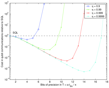
Figure 1: Resources requirements of the improved protocol relative to the simple protocol (SQL) for several values of channel efficiency.

Figure 1 shows a comparison of the relative cost (in terms of qubit communications) of the improved protocol compared with the simple protocol (SQL) with the same noise. The improved protocol beats the SQL for low precisions, even in the presence of small amounts of loss in the channel. Performance falls off for high precisions at a threshold dependent on the channel quality. The observed behaviour is that the maximum number of bits of precision scales as $k_{\rm max}\sim\ln(1-\eta)$. The improved protocol will beat the SQL for a range of precisions, and this range increases with channel quality.

Beyond the point where the improved protocol no longer beats the SQL, one can use a “hybrid” algorithm, which uses the improved protocol to estimate the first $k_{1}$ bits of precision and then it switches to a simple protocol to estimate the remaining $k-k_{1}$ bits. However, in the simple protocol phase, each qubit can be communicated $2^{k_{1}}$ times before the measurement is performed instead of just once, yielding an effective qubit frequency of $2^{k_{1}}\omega$. The performance of such a protocol will scale as the improved protocol up to $k_{1}$ bits of precision, and then scale as the SQL (albeit with a higher effective frequency) once the simple protocol takes over. Thus the performance relative to the SQL is constant for precisions of $k_{1}$ and higher.

As an example, future optical clock standards such as those described in Takamoto et al. Tak05 using Sr atoms with a transition frequency of 429 THz, are predicted to have a fractional time uncertainty of one part in $10^{18}$. Suppose we wish to synchonize two such clocks, every second, and thus require synchronization to $10^{-18}$ seconds. In principle, synchronization can be achieved via the exchange of Sr atoms (or any ticking qubits operating at this optical frequency, such as optical photons), requiring $k=11$ bits of precision in $T$. For channel transmission coefficients of 0.9, 0.99, and 0.999, the “hybrid” algorithm beats the SQL by factors of 7, 60 and 400 respectively in qubit communication cost. Alternatively, exchange of qubits ticking at RF frequency (such as Cs atoms using the standard 9 192 631 770 Hz transition) would require $k=26$ bits of precision in $T$. The performance relative to the SQL remains approximately the same in this case, due to the channel noise forbidding operation at the Heisenberg limit beyond a precision $k_{\rm max}\sim\ln(1-\eta)$.

VI Discussion

We have presented an analysis of “ticking qubit” protocols for clock synchronization, based on the Eddington slow clock transport protocol. We have demonstrated a simple protocol that through $N_{c}$ independent one-way qubit communications achieves the “standard quantum limit” scaling of $\Delta t_{BA}\sim 1/(\omega\sqrt{N_{c}})$. This limit can be beaten by an improved protocol, which requires multiple coherent communications of a qubit, but makes no use of entanglement and gives $\Delta t_{BA}\sim(\omega N_{c})^{-1}\log N_{c}$. This result is in contrast with a standard assumption that entanglement is required to beat the standard quantum limit.

Inspection of (27) reveals that our improved protocol gives us a way of effectively increasing the qubit ticking frequency. By coherently exchanging a qubit back and forth $M$ times, interspersed with each party’s $X_{P}$ operation, we produce an effective ticking frequency of $M\omega$, precisely like a single exchange of an $M$-qubit entangled state. Thus, we have the following three-way equivalence in resources for clock synchronization in terms of the measurement statistics they generate:

1. sending a single qubit ticking at frequency $M\omega$;

2. sending an $M$-qubit entangled state of the form of Eq. (31), with each qubit at frequency $\omega$;

3. $M$ two-way coherent communications of a single qubit at frequency $\omega$.

If we consider the number of qubit communications as determining the cost of a protocol, then we find that techniques (2) and (3) are equivalent, while (1) gives an improvement by a factor of $M$. Clearly, there is enormous advantage to possessing qubits with larger frequencies, as was demonstrated in the second protocol of Chuang Chu00 . The use of coherent communications as a substitute for sending multiple-qubit entangled states in quantum information protocols, first suggested in Rud03 , has been largely unexplored.

Finally, we found that the improved protocol can function in the presence of noise (a lossy channel). While the noise limits the maximum precision, it is still possible to beat the standard quantum limit.

- (1) I. L. Chuang, Phys. Rev. Lett. 85, 002006 (2000).
- (2) R. Jozsa, D. S. Abrams, J. P. Dowling, and C. P. Williams, Phys. Rev. Lett. 85, 002010 (2000); E. A. Burt, C. R. Ekstrom, and T. B. Swanson Phys. Rev. Lett. 87, 129801 (2001); R. Jozsa, D. S. Abrams, J. P. Dowling, and C. P. Williams, Phys. Rev. Lett. 87, 129802 (2001).
- (3) J. Preskill, arXiv:quant-ph/0010098.
- (4) V. Giovannetti, S. Lloyd, and L. Maccone, Nature (London) 412, 417 (2001).
- (5) V. Giovannetti, S. Lloyd, and L. Maccone, Phys. Rev. A65, 022309 (2002).
- (6) U. Yurtsever and J. P. Dowling, Phys. Rev. A65, 052317 (2002).
- (7) V. Giovannetti, S. Lloyd, L. Maccone, J. H. Shapiro, and F. N. C. Wong, Phys. Rev. A70, 043808 (2004).
- (8) A. Valencia, G. Scarcelli, and Y. Shih, Appl. Phys. Lett. 85, 2655 (2004).
- (9) V. Giovannetti, S. Lloyd, and L. Maccone, Science 306, 1330 (2004).
- (10) A. Einstein, Ann. Phys. 17, 891 (1905); Einstein, The Swiss Years: Writings, 1900-1909 (Princeton University Press, Princeton, NJ, 1989), Vol 2, pp. 140-171.
- (11) A. S. Eddington, The Mathematical Theory of Relativity (Cambridge University Press, Cambridge, 1924).
- (12) E. Samain and P. Fridelance, Metrologia, 35, 151 (1998).
- (13) M. A. Nielsen and I. L. Chuang, Quantum Computation and Quantum Information, (Cambridge University Press, Cambridge, 2000).
- (14) M. J. Fitch and J. D. Franson, Phys. Rev. A65, 053809 (2002).
- (15) V. Giovannetti, S. Lloyd, L. Maccone, J. H. Shapiro and F. N. C. Wong, Phys. Rev. A70, 043808 (2004).
- (16) C. M. Caves, Phys. Rev. D23, 1693 (1981).
- (17) B. Yurke, S. L. McCall, and J. R. Klauder, Phys. Rev. A33, 4033 (1986).
- (18) M. J. Holland and K. Burnett, Phys. Rev. Lett. 71, 1355 (1993).
- (19) B. C. Sanders and G. J. Milburn, Phys. Rev. Lett. 75, 2944 (1995).
- (20) J. J. Bollinger, W. M. Itano, D. J. Wineland, and D. J. Heinzen, Phys. Rev. A54, R4649 (1996).
- (21) D. W. Berry and H. M. Wiseman, Phys. Rev. Lett. 85, 5098 (2000).
- (22) A. Peres and P. F. Scudo, Phys. Rev. Lett. 86, 4160 (2001).
- (23) E. Bagan, M. Baig, A. Brey, R. Muñoz-Tapia and R. Tarrach, Phys. Rev. A63, 052309 (2001).
- (24) T. Rudolph and L. Grover, Phys. Rev. Lett. 91, 217905 (2003).
- (25) M. W. Mitchell, J. S. Lundeen, and A. M. Steinberg, Nature (London), 429, 161 (2004).
- (26) D. Leibfried, M. D. Barrett, T. Schaetz, J. Britton, J. Chiaverini, W. M. Itano, J. D. Jost, C. Langer, and D. J. Wineland, Science 304, 1476 (2004).
- (27) C. A. Sackett, D. Kielpinski, B. E. King, C. Langer, V. Meyer, C. J. Myatt, M. Rowe, Q. A. Turchette, W. M. Itano, D. J. Wineland and C. Monroe, Nature (London) 404, 256 (2000).
- (28) P. Walther, J.-W. Pan, M. Aspelmeyer, R. Ursin, S. Gasparoni, and A. Zeilinger, Nature (London), 429, 158 (2004).
- (29) H. M. Wiseman, in Fluctuations and Noise in Photonics and Quantum Optics, Proc. SPIE, Vol. 5111, edited by D. Abbott, J. H. Shapiro, and Y. Yamamoto (SPIE, Bellingham, WA, 2003), pp 78-91.
- (30) H. M. Wiseman, J. Opt. B: Quantum Semiclassical Opt. 6, 5849 (2004).
- (31) J. I. Cirac and P. Zoller, Phys. Rev. Lett. 74, 4091 (1995).
- (32) S. D. Bartlett, T. Rudolph and R. W. Spekkens, Phys. Rev. Lett. 91, 027901 (2003).
- (33) S. J. van Enk, Phys. Rev. A71, 032339 (2005).
- (34) J. I. Cirac, L. M. Duan, and P. Zoller, in Experimental Quantum Computation and Information, Proceedings of the International School of Physics “Enrico Fermi”, Course CXLVIII, p. 263, edited by F. Di Martini and C. Monroe (IOS Press, Amsterdam, 2002), arXiv:quant-ph/0405030.
- (35) M Takamoto, F Hong, R Higashi and H Katori, Nature (London) 435, 321 (2005).