A two-level atom coupled to a controllable squeezed vacuum field reservoir

Abstract

The dissipative and decoherence properties of the two-level atom interacting with the squeezed vacuum field reservoir are investigated based on the nonautonomous master equation of the atomic density matrix in the framework of algebraic dynamics. The nonautonomous master equation is converted into a Schrödinger-like equations and its dynamical symmetry is found based on the left and right representations of the relevant algebra. The time-dependent solution and the steady solution are obtained analytically. The asymptotic behavior of the solution is examined and the approach to the equilibrium state is proved. Based on the analytic solution the response of the system to the squeezed vacuum field reservoir is studied numerically.

I Introduction

The fundamental property of the squeezed state is that the quantum fluctuations in one quadrature component of the field can be reduced heavily. Followed the early works pleb ; yue , much attention has been given to this specific state. The first experimental result for the generation of the squeezed state was reported by Slusher et al.slu with the scheme of 4-wave mixing in an optical cavity. Currently a successful scheme for generating squeezed light can also be based on a parametric oscillator or parametric down converter pozik . Recently, due to its potential applications in the fields of quantum measurement, optical communication, and quantum information, the squeezed vacuum state has been extensively studied Fur ; Hau . A natural problem is what effect on physical systems can be induced by the squeezed vacuum. The squeezed light field will generally be characterized as a non-stationary reservoir which contains phase dependent features in the correlation function between pairs of photons. When the bandwidths of the squeezed lights are not too small, they can be treated as Markovian reservoirs, and the master equations of the reduced system can be obtained based on Markovian approximation.

Master equations are of fundamental importance in the treatment of dissipation and decoherence of open quantum systems. The common feature of the quantum master equations is the existence of the sandwich terms of the Liouville operators where the reduced density matrix of the system is in between some quantum excitation and de-excitation operators. So it is very difficult to get the exact analytical solution of the master equation, only simple cases such as a single mode of cavity field coupled to a vacuum state reservoir ($T=0$) or stationary regime properties are the ones analytically treated Scu . Instead, the master equations are normally converted into c-number equations in the coherent state representation–the Fokker-Planck equation Gar ; Wall . On the other hand, with the development of the so called quantum engineering, the man-made nonautonomous quantum systems where the system parameters set by people for controlling of the system are time-dependent, become more and more important. It would be very desirable to get the analytical solution of the corresponding master equation of such a system. Further, even if the total Hamiltonian of an open system-a system plus an environment, is time-independent, the master equation of the reduced density matrix of the investigated system still becomes nonautonomous under the non-Markovian dynamics Ana . Therefore, quantum master equation of the reduced density matrix, in general, should be nonautonomous.

In the previous works Zhao ; Wang01 ; An , we have proposed and developed an algebraic method to treat the sandwich terms in the Liouville operator for the nonequilibrium quantum process. This method is just a generalization of the algebraic dynamical method Wang93 from quantum mechanical systems to quantum statistical ones. According to the characteristic of the sandwich terms in the Liouville operator, the left and right representations Wang89 of the relevant algebra have been introduced and the corresponding composite algebra has been constructed. As a result, the master equation has been converted into a Schrödinger-like equation and the problems can be solved exactly in the framework of algebraic dynamics. This method is very effective to treat the nonautonomous quantum system which contains time-dependent parameters for control of the system.

In this paper, using the algebraic dynamical method, we shall solve the problem of two-level atom interacting with the squeezed vacuum field reservoir and investigate what effect on the system can be induced by the squeezed vacuum field reservoir. As is well known, when the environment is ordinary thermal equilibrium fields, the model, either be autonomous or be nonautonomous, has been investigated very well Gar ; An . When the environment is the squeezed vacuum field, some work have been done on this field phase ; Dalt . Different to Ref. Dalt , where two-level atoms with a time-dependent external classical driven field in the squeezed vacuum field reservoir were investigated, in this paper, we will concentrate on the behavior of a two-level atom in a time-dependent squeezed vacuum field reservoir. With the help of the algebraic dynamical method, the $su(2)\oplus su(2)$ dynamical symmetry of the nonautonomous master equation for the two-level atom is found. The analytical solutions, both the steady solutions and the time-dependent solutions of the system are obtained exactly, and the decay property of the atom is investigated. For the asymptotic behavior of the system, it is proven that any time-dependent solution of the system approaches its unique steady equilibrium solution. Based on the analytical solution, the different response behaviors of the system to the time-dependent squeezing parameter $r$, linear and nonlinear, are investigated numerically. We noticed that in the nonlinear response regime, the expectation of one of the squeezed components of the system, $\sigma_{y}$, is much enhanced, and the squeezed property of the system, i.e., the asymmetry of the decay of the expectation of $\sigma_{x}$ and $\sigma_{y}$, can also be manifested even when the initial values of $\sigma_{i}$ ($i=x,y$) are zero.

The paper is organized as follows. In section II, the model Hamiltonian of the system is presented and the master equation for the reduced matrix of the atom is deduced. In section III, the dynamical $su(2)_{K}\oplus su(2)_{J}$ algebraic structure of the Liouville operator of the master equation is found and the dynamical symmetry of the system is thus exposed. Section IV is devoted to obtain the analytical non-equilibrium solution of the nonautonomous master equation, and the approach to the unique steady equilibrium solution asymptotically is proved. In section V, numerical results are presented for illustration of non-equilibrium process of some physical quantities. Discussions and conclusions are given in the final section.

II A two-level atom in the squeezed vacuum field reservoir

The Hamiltonian of a two-level atom interacting with a squeezed vacuum field reservoir is

$$\hat{H}=\frac{1}{2}\hbar\omega_{0}\sigma_{z}+\hbar\sum_{k}\omega_{k}(a_{k}^{\dagger}a_{k}+\frac{1}{2})+\hbar\sum_{k}g_{k}(\sigma_{+}a_{k}+h.c.),$$

Since the squeezed vacuum field reservoir is kept fixed, the total density operator of the system can be written as Scu

$$\rho_{T}(t)=\rho\left(t\right)\otimes\prod_{k}S_{k}\left(\xi\right)|0_{k}\rangle\langle 0_{k}|S_{k}^{\dagger}\left(\xi\right),$$

where $S_{k}\left(\xi\right)$ is the squeezing operator and reads as

$$S_{k}\left(\xi\right)=\exp(\xi^{\ast}a_{k_{0}+k}a_{k_{0}-k}-\xi a_{k_{0}+k}^{\dagger}a_{k_{0}-k}^{\dagger})$$

with $\omega=ck_{0}$ and $\xi=r\exp\left(i\theta\right)$, $r$ being the squeezing parameter and $\theta$ being the reference phase for the squeezed field. Then the master equation for the reduced density matrix $\rho\left(t\right)$ of the atom interacting with the squeezed vacuum reservoir can be obtained with the standard Markovian approximation Scu ,

$$\dot{\rho} = \frac{\gamma}{2}\ (N+1)\ (2\sigma_{-}\rho\sigma_{+}-\sigma_{+}\sigma_{-}\rho-\rho\sigma_{+}\sigma_{-})$$ (1)

$$+\frac{\gamma}{2}\ N\ (2\sigma_{+}\rho\sigma_{-}-\sigma_{-}\sigma_{+}\rho-\rho\sigma_{-}\sigma_{+})$$

$$-\gamma M\sigma_{-}\rho\sigma_{-}-\gamma M^{\ast}\sigma_{+}\rho\sigma_{+},$$

where $\langle a_{k}^{\dagger}a_{k^{\prime}}\rangle=N\delta_{kk^{\prime}}=\sinh^{2}(r)\delta_{kk^{\prime}}$, $\langle a_{k}^{\dagger}a_{k^{\prime}}^{\dagger}\rangle=-M\delta_{k^{\prime},2k_{0}-k}=-\cosh\left(r\right)\sinh\left(r\right)\exp\left(-i\theta\right)\delta_{k^{\prime},2k_{0}-k}$, and $N$ is very large. Here we have assumed that the vacuum field reservoir is the ideal squeezed one, that is, $M^{2}=N(N+1)$. When $N\rightarrow\bar{n}=<\frac{1}{\exp(\frac{\hbar\nu_{k}}{k_{B}T})+1}><<1$, $M\rightarrow 0$, the master equation (1) reduces to the familiar form of the master equation An describing an two-level atom coupling to the ordinary thermal equilibrium radiation field. The last two terms of the above equation exhibit the phase-sensitive nature of the investigated system. The autonomous case of this equation can be found in phase , while in this paper we concentrate on the nonautonomous case where all the parameters $M$, $N$ and, $\gamma$ of Eq. (1) are time-dependent, which allow for adjustment of the squeezing parameter $r$, the reference phase $\theta$, and the coupling parameter $g_{k}$ during the time.

III Dynamical symmetry of the master equation

First we will explore the algebraic structure of Eq. (1). Based on the left and right representations of certain algebra Wang01 , we can get the right and left representations of the algebra $su\left(2\right)=\{\sigma_{+},\sigma_{-},\sigma_{z}\}$

$$su\left(2\right)_{r} : [\sigma_{z}^{r},\sigma_{\pm}^{r}]=\pm 2\sigma_{\pm}^{r},\;\;[\sigma_{+}^{r},\sigma_{-}^{r}]=\sigma_{z}^{r},$$

$$su\left(2\right)_{l} : [\sigma_{z}^{l},\sigma_{\pm}^{l}]=\mp 2\sigma_{\pm}^{l},\;\;[\sigma_{+}^{l},\sigma_{-}^{l}]=-\sigma_{z}^{l}.$$ (2)

It is evident that $su(2)_{r}$ is isomorphic to the $su(2)$, while $su(2)_{l}$ anti-isomorphic to the $su(2)$. This is because $su(2)_{r}$ operates towards the right on the bra space $|\ \rangle$; but on the other hand, $su(2)_{l}$ operates on the ket space $\langle\ |$. Just for the reason that $su(2)_{r}$ and $su(2)_{l}$ operate on different spaces(the dual bra and ket spaces), they commute with each other, i.e.

$$[su(2)_{r},su(2)_{l}]=0.$$ (3)

From these basic representations of $su\left(2\right)$ we can constitute two composite algebras

$$su(2) : \{J_{0}=\frac{\sigma_{z}^{r}+\sigma_{z}^{l}}{2},J_{+}=\sigma_{+}^{r}\sigma_{-}^{l},J_{-}=\sigma_{-}^{r}\sigma_{+}^{l}\},$$

$$su\left(2\right) : \{K_{0}=\frac{\sigma_{z}^{r}-\sigma_{z}^{l}}{2},K_{+}=\sigma_{+}^{r}\sigma_{+}^{l},K_{-}=\sigma_{-}^{r}\sigma_{-}^{l}\}.$$

According to Eqs. (2) and Eq. (3) it’s straightforward to check the following two $su(2)$ commutation relations

$$[J_{0},J_{\pm}] = \pm 2J_{\pm},\;\;[J_{+},J_{-}]=J_{0},$$

$$[K_{0},K_{\pm}] = \pm 2K_{\pm},\;\;[K_{+},K_{-}]=K_{0},$$

$$[J_{i},K_{j}] = 0\ \ \ (i,j=0,\pm).$$

These two $su(2)$ generators have the action on the bases of von-Neumann space, which span the basis of the atomic density matrix

$$J_{0}|s\rangle\langle s^{\prime}| = \frac{s+s^{\prime}}{2}|s\rangle\langle s^{\prime}|,$$

$$J_{+}|s\rangle\langle s^{\prime}| = \delta_{s+1,0}\delta_{s^{\prime}+1,0}|s+2\rangle\langle s^{\prime}+2|,$$

$$J_{-}|s\rangle\langle s^{\prime}| = \delta_{s-1,0}\delta_{s^{\prime}-1,0}|s-2\rangle\langle s^{\prime}-2|,$$

$$K_{0}|s\rangle\langle s^{\prime}| = \frac{s-s^{\prime}}{2}|s\rangle\langle s^{\prime}|,$$

$$K_{+}|s\rangle\langle s^{\prime}| = \delta_{s+1,0}\delta_{s^{\prime}-1,0}|s+2\rangle\langle s^{\prime}-2|,$$

$$K_{-}|s\rangle\langle s^{\prime}| = \delta_{s-1,0}\delta_{s^{\prime}+1,0}|s-2\rangle\langle s^{\prime}+2|,$$ (4)

where $s(s^{{}^{\prime}})=\pm 1$.

By virtue of the above algebras, the nonautonomous master equation (1) can be rewritten as a linear combination of these generators

$$\dot{\rho}=\gamma\left(t\right)\{[N(t)+1]J_{-}+N(t)J_{+}-\frac{1}{2}J_{0}-M(t)K_{-}-M^{\ast}(t)K_{+}-\frac{2N\left(t\right)+1}{2}\}\rho=\Gamma\rho.$$ (5)

which implies that Eq. (1) possesses an $su\left(2\right)_{J}\oplus su\left(2\right)_{K}$ dynamical symmetry. Thus it is integrable and can be solved analytically according to algebraic dynamics Wang93 . Moreover, the master equation (1) is converted into a Schrödinger-like equation (5), where the rate operator $\Gamma$ plays the role of the Hamiltonian and the reduced matrix plays the role of the wavefunction.

It is noted that Eq. (5) is a time-dependent generalization of Eq. (1) and it is still under the Markovian approximation. That implies a basic assumption: the time dependence of the parameters of the master equation don’t alter the base of the Markovian approximation-the weak coupling assumption of the system and the reservoir.

IV Exact solution to the master equation in the nonautonomous case

IV.1 Steady solution of the master equation

To better understand the time-dependent solution of the master equation and its decay behavior, we first consider the long-time case $\left(\gamma\left(t\right)\rightarrow\gamma,N(t)\rightarrow N,M(t)\rightarrow M\right)$ and the eigen equation problem of the master equation (5). From Eq. (5) we can get

$$\ \Gamma\rho=\beta\rho$$ (6)

Introducing the similarity transformation

$$U=e^{\alpha_{+}J_{+}}e^{\alpha_{-}J_{-}}e^{\eta_{+}K_{+}}e^{\eta_{-}K_{-}},$$

and under the transformation parameter conditions

$$(N+1)\alpha_{+}^{2}+\alpha_{+}-N = 0,$$

$$(N+1)(1+2\alpha_{+}\alpha_{-})+\alpha_{-} = 0,$$ (7)

$$M\eta_{+}^{2}-M^{\ast} = 0,$$

$$\ 1+2\eta_{+}\eta_{-} = 0,$$ (8)

we can transform Eq. (6) to the diagonal form as

$$\bar{\Gamma}\bar{\rho} = \beta\bar{\rho},$$

$$\bar{\rho} = U^{-1}\rho,$$

$$\bar{\Gamma} = U^{-1}\Gamma U=-\gamma\{[(N+1)\alpha_{+}+\frac{1}{2}]J_{0}-M\eta_{+}K_{0}+\frac{2N+1}{2}\}.$$ (9)

The eigensolutions of  Eq. (6) are

$$\beta(s,s^{\prime}) = -\gamma\{[(N+1)\alpha_{+}+\frac{1}{2}]\frac{s+s^{{}^{\prime}}}{2}-M\eta_{+}\frac{s-s^{{}^{\prime}}}{2}+\frac{2N+1}{2}\},$$

$$\rho(s,s^{\prime}) = e^{\alpha_{+}J_{+}}e^{\alpha_{-}J_{-}}e^{\eta_{+}K_{+}}e^{\eta_{-}K_{-}}|s\rangle\langle s^{\prime}|.$$ (10)

It is interesting to note that Eqs. (7) and Eqs. (8) both have two sets of solutions. The two combinations of the solutions $(\alpha_{+}=-1,\ \alpha_{-}=(N+1)/(2N+1),\ \eta_{+}=\pm e^{i\theta},\$and $\eta_{-}=\mp e^{-i\theta})$ and $(\alpha_{+}=N/(2N+1),\ \alpha_{-}=-(N+1)/(2N+1),\ \eta_{+}=\pm e^{i\theta},\$and $\eta_{-}=\mp e^{-i\theta})$ both contain the same zero-mode solution (the unique steady equilibrium solution) and they are equivalent physical solutions since all their eigen values $\beta(s,s^{\prime})$ are non-positive (this can be proved by the series expansion $M=\sqrt{N(N+1)}\approx N(1+\frac{1}{2N}-\frac{1}{8N^{2}})$ and by the fact $N\pm M+\frac{1}{2}>0$).

Noticing that $J_{\pm}$ yield non-zero results only if they act on diagonal elements and $K_{\pm}$ do so if they act on non-diagonal elements, we see that the zero mode steady solution of the system has the same form (but with different $N$) as that in Ref. An where the reservoir is a thermal equilibrium field,

$$\rho_{0}=\frac{N+1}{2N+1}|-1\rangle\langle-1|+\frac{N}{2N+1}|+1\rangle\langle+1|,$$ (11)

It is noted that the rate operator $\Gamma$ is non-Hermitian, i.e. $\Gamma^{\dagger}\neq\Gamma$, which is evident from $J_{+}^{\dagger}=J_{-}$, $J_{-}^{\dagger}=J_{+}$, $J_{0}^{\dagger}=J_{0}$, $K_{+}^{\dagger}=K_{-}$, and $K_{-}^{\dagger}=K_{+}$. Just because of this non-Hermiticity, the eigenvectors of $\Gamma$ and $\Gamma^{\dagger}$ constitute a bi-orthogonal basis Feshbach . By introducing a similarity transformation $U^{\prime}=(U^{-1})^{\dagger}$ and umder the same conditions as Eqs. (7, 8), the operator $\Gamma^{\dagger}$ can be diagonalized. Then the eigensolutions of $\Gamma^{\dagger}$ are given by

$$\Gamma^{\dagger}\tilde{\rho}(s,s^{\prime}) = \tilde{\beta}(s,s^{\prime})\tilde{\rho}(s,s^{\prime})$$

$$\tilde{\beta}(s,s^{\prime}) = \beta^{\ast}(s,s^{\prime})$$

$$\tilde{\rho}(s,s^{\prime}) = e^{-\eta_{+}K_{-}}e^{-\eta_{-}K_{+}}e^{-\alpha_{+}J_{-}}e^{-\alpha_{-}J_{+}}|s\rangle\langle s^{\prime}|.$$ (12)

One can easily to check that the eigenvectors $\rho(s,s^{\prime})$ and $\tilde{\rho}(s,s^{\prime})$ form a biorthogonal set. A similar discussion can be found in Ref. An .

To compare with the work of Ref. Briegel ; Sten ; Jakob , we consider the left eigensolutions of $\Gamma$. The transformed form of the eigen equation is

$$\bar{\rho}^{\prime}\bar{\Gamma}=\beta^{\prime}(s,s^{\prime})\bar{\rho}^{\prime}$$

Eq. (9) shows that the operator $\bar{\Gamma}=U^{-1}\Gamma U$ is self-adjoint and, thus, $\bar{\rho}^{\prime}\bar{\Gamma}=U^{\dagger}\Gamma^{\dagger}(U^{-1})^{\dagger}\bar{\rho}^{\prime}=[(U^{-1})^{\dagger}]^{-1}\Gamma^{\dagger}(U^{-1})^{\dagger}\bar{\rho}^{\prime}$. This implies that $\Gamma^{\dagger}$ has the same eigensolutions as $\Gamma$ when they act from the left and right on $\rho$, respectively. In the phrase of Ref. Briegel , $\rho(s,s^{\prime})$ is the right-hand eigenvectors of the operator $\Gamma$ and $\tilde{\rho}(s,s^{\prime})$ is the right-hand eigenvectors of the operator $\Gamma^{\dagger}$. Furthermore the right-hand eigenvectors of the operator $\Gamma^{\dagger}$ coincide with the left-hand eigenvectors of $\Gamma$. And the two sets of eigenvectors constitute a biorthogonal set. From this biorthogonal set one can construct a generalized entropy functional varying monotonically with time, which named as the Lyapunov functional and have a crucial rules in control theory Jakob .

IV.2 Time-dependent solution of the master equation

Now we turn back to the nonautonomous case and study the time-dependent solution of Eq. (5). With the gauge transformation

$$U_{g}\left(t\right)=e^{\alpha_{+}\left(t\right)J_{+}}e^{\alpha_{-}\left(t\right)J_{-}}e^{\eta_{+}\left(t\right)K_{+}}e^{\eta_{-}\left(t\right)K-},$$

and the gauge parameters satisfying

$$\frac{d\alpha_{+}(t)}{dt} = -\gamma(t)[N(t)+1]\alpha_{+}^{2}(t)-\gamma(t)\alpha_{+}(t)+\gamma(t)N(t),$$

$$\frac{d\alpha_{-}(t)}{dt} = \gamma(t)[N(t)+1][1+2\alpha_{+}(t)\alpha_{-}(t)]+\gamma(t)\alpha_{-}(t),$$

$$\frac{d\eta_{+}\left(t\right)}{dt} = \gamma(t)[M(t)\eta_{+}^{2}\left(t\right)-M^{\ast}(t)],$$

$$\frac{d\eta_{-}\left(t\right)}{dt} = -\gamma(t)M(t)[1+2\eta_{+}\left(t\right)\eta_{-}\left(t\right)].$$ (13)

where the initial conditions of the gauge transformation is $U_{g}(0)=1$, the operator $\Gamma$ can be transformed to the diagonal form

$$\bar{\Gamma}\left(t\right) = U_{g}^{-1}\left(t\right)\Gamma U_{g}\left(t\right)-U_{g}^{-1}\left(t\right)\dot{U}_{g}\left(t\right)$$

$$= -\gamma(t)\{[(N\left(t\right)+1)\alpha_{+}\left(t\right)+\frac{1}{2}]J_{0}-M\left(t\right)\eta_{+}\left(t\right)K_{0}+\frac{2N\left(t\right)+1}{2}\}$$

If the initial state of the system is $\rho\left(0\right)=\sum_{s,s^{\prime}}\lambda_{s,s^{\prime}}|s\rangle\langle s^{\prime}|$, then the time-dependent solution of the nonautonomous master Eq. (5) is

$$\rho\left(t\right) = \sum_{s,s^{\prime}}\lambda_{s,s^{\prime}}U_{g}\left(t\right)e^{\int_{0}^{t}-\gamma(\tau)\{[(N\left(\tau\right)+1)\alpha_{+}\left(\tau\right)+\frac{1}{2}]\frac{s+s^{\prime}}{2}-M\left(\tau\right)\eta_{+}\left(\tau\right)\frac{s-s^{\prime}}{2}+\frac{2N\left(\tau\right)+1}{2}\}d\tau}|s\rangle\langle s^{\prime}|$$ (14)

$$= \{\lambda_{1,1}f_{1,1}(t)[1+\alpha_{+}\left(t\right)\alpha_{-}(t)]+\lambda_{-1,-1}f_{-1,-1}(t)\alpha_{+}\left(t\right)\}|+1\rangle\langle+1|$$

$$+[\lambda_{1,1}f_{1,1}(t)\alpha_{-}(t)+\lambda_{-1,-1}f_{-1,-1}(t)]|-1\rangle\langle-1|$$

$$+\{\lambda_{1,-1}f_{1,-1}(t)[1+\eta_{+}\left(t\right)\eta_{-}(t)]+\lambda_{-1,1}f_{-1,1}(t)\eta_{+}\left(t\right)\}|+1\rangle\langle-1|$$

$$+[\lambda_{1,-1}f_{1,-1}(t)\eta_{-}(t)+\lambda_{-1,1}f_{-1,1}(t)]|-1\rangle\langle+1|,$$

where we have defined $f_{s,s^{\prime}}(t)=e^{\int_{0}^{t}-\gamma(\tau)\{[(N\left(\tau\right)+1)\alpha_{+}\left(\tau\right)+\frac{1}{2}]\frac{s+s^{\prime}}{2}-M\left(\tau\right)\eta_{+}\left(\tau\right)\frac{s-s^{\prime}}{2}+\frac{2N\left(\tau\right)+1}{2}\}d\tau}$.

One can check that the solution of Eq. (14) recovers the results of the autonomous system with time-independent parameters. For the autonomous case, the explicit solutions of the gauge parameters $\alpha_{\pm}$ and $\eta_{\pm}$ can be obtained from Eqs. (13)

$$\alpha_{+}(t) = \frac{1-e^{-\gamma(2N+1)t}}{\frac{N+1}{N}+e^{-\gamma(2N+1)t}},$$

$$\alpha_{-}(t) = \frac{(N+1)N[\frac{N+1}{N}+e^{-\gamma(2N+1)t}][1-e^{-\gamma(2N+1)t}]}{(2N+1)^{2}e^{-\gamma(2N+1)t}}.$$

$$\eta_{+}(t) = \frac{1-e^{2\gamma Mt}}{1+e^{2\gamma Mt}},$$

$$\eta_{-}(t) = \frac{(1-e^{2\gamma Mt})(1+e^{2\gamma Mt})}{4e^{2\gamma Mt}},$$

where $M=M^{\ast}$ is assumed. Then under the initial condition of the system

$$\rho\left(0\right)=|\mu|^{2}|1\rangle\langle 1|+|\nu|^{2}|-1\rangle\langle-1|+\mu\nu^{\ast}|1\rangle\langle-1|+\mu^{\ast}\nu|-1\rangle\langle 1|,$$ (15)

the expectation values of $\sigma_{x}$, $\sigma_{y}$, and $\sigma_{z}$ are

$$\langle\sigma_{x}\rangle = (\mu\nu^{\ast}+\mu^{\ast}\nu)e^{-\gamma(N+M+\frac{1}{2})t},$$

$$\langle\sigma_{y}\rangle = \frac{1}{i}(\mu^{\ast}\nu-\mu\nu^{\ast})e^{-\gamma(N-M+\frac{1}{2})t},$$

$$\langle\sigma_{z}\rangle = \frac{2[|\mu|^{2}(N+1)-|\nu|^{2}N]e^{-\gamma(2N+1)t}-1}{2N+1}.$$ (16)

So the decoherent characteristic times of $\langle\sigma_{x}\rangle$, $\langle\sigma_{y}\rangle$, and $\langle\sigma_{z}\rangle$ are $\frac{1}{\gamma(N+M+\frac{1}{2})},$ $\frac{1}{\gamma(N-M+\frac{1}{2})},$and $\frac{1}{\gamma(2N+1)}$, respectively, which is same as the results of Ref. phase . The decoherent characteristic time of $\langle\sigma_{y}\rangle$ is much larger than that of $\langle\sigma_{x}\rangle$. From the above results we see that the radiative properties of the atom depend sensitively on the state of the environment to which it is coupled. The squeezed vacuum reservoir imposes its phase information on the atom and makes a highly asymmetric decay property of the atom. This is quite different from thermal vacuum reservoir which results in the same decay rate (where $M=0$, $N\rightarrow\bar{n}$) for $\langle\sigma_{y}\rangle$ and $\langle\sigma_{x}\rangle$.

So we can see that the time-dependent solution of Eq. (14) reproduces all the results of the autonomous case. In the following we shall concentrate on the nonautonomous case and investigate the time evolution behaviors of the system.

IV.3
The asymptotical behavior of the solution

In this section we shall examine the asymptotic behavior of the time-dependent analytical solution (14) of the nonautonomous master equation and prove that it approaches to the equilibrium steady solution (11). To this end we shall first investigate the asymptotic behavior of the gauge parameters which are solutions of Eqs. (13) from which one notices that $d\eta_{+}(t)/dt<0(>0)$ if $-1<\eta_{+}(t)<0$ (if $\eta_{+}(t)<-1$ and $\eta_{+}(t)>0$). With the initial condition $\eta_{+}\left(0\right)=0$, we see that $\eta_{+}\left(t\right)$ approaches the value $\eta_{+}\left(\infty\right)=-1$ asymptotically. To get the asymptotic solution of $\eta_{-}\left(t\right)$, we define $y(t)=\eta_{-}\left(t\right)e^{\int_{0}^{t}2\gamma(\tau)M\left(\tau\right)\eta_{+}\left(\tau\right)d\tau}=\eta_{-}\left(t\right)e^{\int_{0}^{t}p\left(\tau\right)d\tau}$. The time differential of $y\left(t\right)$ is given by $b\exp\int_{0}^{t}p(\tau)d\tau$ where $b=\dot{\eta}_{-}(t)+\eta_{-}(t)p(t)$. Since $b\longrightarrow\gamma$ which is bounded and $p(t)$ is negative for large $t$, the differential $\dot{y}\left(t\right)$ tends to zero, hence $y\left(t\right)$ tends towards a constant. With the same procedure we can get the asymptotic solutions of $\alpha_{\pm}\left(t\right)$. Summarizing the above discussion, we have

$$\alpha_{+}(t)|_{t\rightarrow\infty} = \frac{N}{N+1}$$

$$\alpha_{-}(t)\times e^{-\int_{0}^{t}\gamma(\tau)[N(\tau)+1][\alpha_{+}(\tau)+1]d\tau}|_{t\rightarrow\infty} = const$$

$$\eta_{+}\left(t\right)|_{t\rightarrow\infty} = -1$$

$$\eta_{-}\left(t\right)e^{\int_{0}^{t}2\gamma(\tau)M\left(\tau\right)\eta_{+}\left(\tau\right)d\tau}|_{t\rightarrow\infty} = const.$$

Although, for the steady case, two sets of the parameter solutions $\alpha_{\pm}$ and $\eta_{\pm}$  lead to two equivalent transformations which diagonalize the rate operator and generate the same physical solution, as discussed above; for the time-dependent case, the properties of the two sets of steady solutions of $\alpha_{\pm}$ and $\eta_{\pm}$ are not on equal footing. It is found that only one set of the solutions can be reached by the time-dependent solution asymptotically. Using these asymptotic relations we have the asymptotic results of the time-dependent solution as follows

$$\rho_{++}(t)|_{t\rightarrow\infty} = e^{-\int_{0}^{t}\gamma(\tau)[N(\tau)+1][\alpha_{+}(\tau)+1]d\tau}[|+1\rangle\langle+1|+\alpha_{-}(t)(|-1\rangle\langle-1|+\alpha_{+}(t)|+1\rangle\langle+1|)]$$

$$\longrightarrow const.\times\rho_{0}$$

$$\rho_{--}(t)|_{t\rightarrow\infty} = e^{-\int_{0}^{t}\gamma(\tau)[-(\bar{n}_{0}(\tau)+1)\alpha_{+}(\tau)+\bar{n}_{0}(\tau)]d\tau}[|-1\rangle\langle-1|+\alpha_{+}(t)|+1\rangle\langle+1|]\longrightarrow const.\times\rho_{0}$$

$$\rho_{+-}(t)|_{t\rightarrow\infty} = e^{-\int_{0}^{t}\gamma(\tau)[M\left(\tau\right)\eta_{+}\left(\tau\right)+N\left(\tau\right)+\frac{1}{2}]d\tau}e^{\int_{0}^{t}2\gamma(\tau)M\left(\tau\right)\eta_{+}\left(\tau\right)d\tau}\{|+1\rangle\langle-1|+\eta_{-}\left(t\right)[\eta_{+}\left(t\right)|+1\rangle\langle-1|+|-1\rangle\langle+1|]\}$$

$$\longrightarrow e^{-\int_{0}^{t}\gamma(\tau)[M\left(\tau\right)+N\left(\tau\right)+\frac{1}{2}]d\tau}|+1\rangle\langle-1|+e^{-\int_{0}^{t}\gamma(\tau)[N\left(\tau\right)-M\left(\tau\right)+\frac{1}{2}]d\tau}\times const[|-1\rangle\langle+1|-|+1\rangle\langle-1|]$$

$$\longrightarrow 0$$

$$\rho_{-+}(t)|_{t\rightarrow\infty} = e^{-\int_{0}^{t}\gamma(\tau)[M\left(\tau\right)\eta_{+}\left(\tau\right)+N\left(\tau\right)+\frac{1}{2}]d\tau}[\eta_{+}\left(t\right)|+1\rangle\langle-1|+|-1\rangle\langle+1|]$$

$$\longrightarrow 0$$

The above results indicate that any time-dependent solution of the master equation in the nonautonomous case asymptotically approaches the unique steady equilibrium solution, irrespective of their initial conditions.

V Numerical results

To study the squeezed properties of the system in the nonautonomous case, we shall start from the time-dependent analytical solution Eq. (14) and calculate the expectation values of the two-level atomic operators. The expectation values of $\sigma_{i}\left(i=x,y,z\right)$ are

$$\langle\sigma_{x}\rangle = \frac{\mu\nu^{\ast}f_{1,-1}[1+\eta_{+}(t)\eta_{-}(t)+\eta_{-}(t)]+\mu^{\ast}\nu f_{-1,1}[1+\eta_{+}(t)]}{2},$$

$$\langle\sigma_{y}\rangle = \frac{\mu\nu^{\ast}f_{1,-1}[1+\eta_{+}(t)\eta_{-}(t)-\eta_{-}(t)]+\mu^{\ast}\nu f_{-1,1}[\eta_{+}(t)-1]}{2i},$$

$$\langle\sigma_{z}\rangle = |\mu|^{2}f_{1,1}[1+\alpha_{+}(t)\alpha_{-}\left(t\right)-\alpha_{-}\left(t\right)]+|\nu|^{2}f_{-1,-1}[\alpha_{+}\left(t\right)-1],$$ (17)

where the initial state is same as Eq. (15). Given any time-dependent parameters $\gamma(t),\ r(t)$, and $\theta(t)$, we can get the gauge transformation parameters $\alpha_{\pm}(t)$ and $\eta_{\pm}$ from Eqs. (13) numerically. Then substitute $\alpha_{\pm}(t)$ and $\eta_{\pm}$ to Eqs. (17), we can obtain the time-dependent behaviors of the expectation values varying according to the system parameters. In the following we will study the variation of the time-dependent behavior of $\langle\sigma_{i}\rangle$ with the squeezing parameter $r(t)$.

Without loss generalization, to explore the time-dependent response of the system to the squeezing parameters we choose time-dependent parameters as $r=c_{1}e^{-c_{2}t}$, $\gamma=1$, and $\theta=0$. Fig. 1 and Fig. 2 show the time-dependent behaviors of $\langle\sigma_{i}\rangle$ with $c_{1}=0.1$ and $c_{2}=0.1$ under the initial condition $\mu=\sqrt{0.2}e^{i/3}$, $\nu=\sqrt{0.8}e^{2\pi i}$ and $\mu=\sqrt{0.2}$, $\nu=\sqrt{0.8}$ respectively. Fig. 3 and Fig. 4 correspond to $c_{2}=0.3$. The behavior of $\langle\sigma_{i}\rangle$ varying to $r(t)$ with parameter $c_{2}=0.6$ were plotted on Fig. 5 and Fig. 6. From these figures we see that $\langle\sigma_{z}\rangle$ decays to its steady value $-1$; $\langle\sigma_{x}\rangle$ and $\langle\sigma_{y}\rangle$ decay to their steady value $0$, but the decay time of $\langle\sigma_{y}\rangle$ is much larger than that of $\langle\sigma_{x}\rangle$, which regenerate the results of the autonomous case. From Fig. 2 we notice that $\langle\sigma_{y}\rangle=0$, so the squeezed property of the squeezed vacuum field to the two-level atom is covered by the initial value of $\langle\sigma_{y}\rangle$. For the small squeezing parameter, the time-dependent response of the system with respect to the squeezing parameter is nearly linear and much like the autonomous case. However, with the increase of squeezing parameter, the response is no longer linear and the decay time of $\langle\sigma_{x}\rangle$’s becomes shorter and shorter, while that of $\langle\sigma_{y}\rangle$’s becomes longer and longer. A more interesting phenomenon appearing during the increase of the squeezing parameter is that the value of $\langle\sigma_{y}\rangle$ can be much enhanced. And the resulting effect of the squeezed vacuum field reservoir on the two-level atom, i.e., the large asymmetric behaviors of decay between $\langle\sigma_{x}\rangle$ and $\langle\sigma_{y}\rangle$, can also be presented even when some of them are zero initially, which is not presented in the autonomous case (this can also be seen from the second expression of Eqs. (16)). Moreover, the time-dependent behavior of $\langle\sigma_{y}\rangle$ is completely different from that of $r(t)$, and the response of system to the squeezing parameter thus exhibits nonlinearity.

From the analysis above we see that the squeezed vacuum field reservoir acts as a squeezing mold and imprint its squeezing information to the two-level atom, which makes the asymmetry of the two decay behaviors. With a time-dependent squeezing parameter this action can be more enhanced, which widen the results of Ref. phase and provide a potential way to get more stable atomic variable. The similar time-dependent system can also be found in Ref. Berg , where a technique of stimulated Raman adiabatic passage was used to get a complete population transfer between two atomic states. There the two adiabatic varying lasers act as a role of coherent trapping in the three-level atomic system and the technique relies on the coherent trapping state.

VI Summary and Outlook

We have investigated the nonautonomous master equation of the two-level atom interacting with the squeezed vacuum reservoir for the first time. The new results of our paper compared to the previous ones are: (1) the dynamical symmetry of the nonautonomous master equation has been established and the master equation has been converted into a Schrödinger-like equation. Based on the dynamical symmetry we have obtained the most general non-equilibrium solutions of the nonautonomous master equation analytically; and as a special case, our solutions recover all the results of the autonomous case. (2) We have proven that any time-dependent and non-equilibrium solution of the nonautonomous master equation approaches its unique steady equilibrium solution asymptotically. (3) The non-equilibrium solution of the nonautonomous master equation is analysed numerically and the different response behaviors of the system to the squeezing parameter is exposed, and nonlinear effect is exhibited.

The works of dissipative system combined with the research of control theory were extended in some publications Jakob ; Sten , how to connect our approach with this investigate is a interesting and challenge problem.

VII Acknowledgment

This work was supported in part by the National Natural Science Foundation of China under grants No.10175029, 10375039, and 10004012, the Doctoral Education Fund of the Education Ministry and Post-doctoral Science Foundation, and the Nuclear Theory Research Fund of HIRFL of China.

Figure 1: The time-dependence of $\langle\sigma_{i}\rangle$ with parameters $r=0.1e^{-0.1t}$, $\mu=\sqrt{0.2}e^{\pi i/3}$, and $\nu=\sqrt{0.8}e^{2\pi i}$.

Figure 2: The time-dependence of $\langle\sigma_{i}\rangle$ with parameters $r=0.1e^{-0.1t}$, $\mu=\sqrt{0.2}$, and $\nu=\sqrt{0.8}$.

Figure 3: The time-dependence of $\langle\sigma_{i}\rangle$ with parameters $r=0.3e^{-0.1t}$, $\mu=\sqrt{0.2}e^{\pi i/3}$, and $\nu=\sqrt{0.8}e^{2\pi i}$.

Figure 4: The time-dependence of $\langle\sigma_{i}\rangle$ with parameters $r=0.3e^{-0.1t}$, $\mu=\sqrt{0.2}$, and $\nu=\sqrt{0.8}$.

Figure 5: The time-dependence of $\langle\sigma_{i}\rangle$ with parameters $r=0.6e^{-0.1t}$, $\mu=\sqrt{0.2}e^{\pi i/3}$, and $\nu=\sqrt{0.8}e^{2\pi i}$.

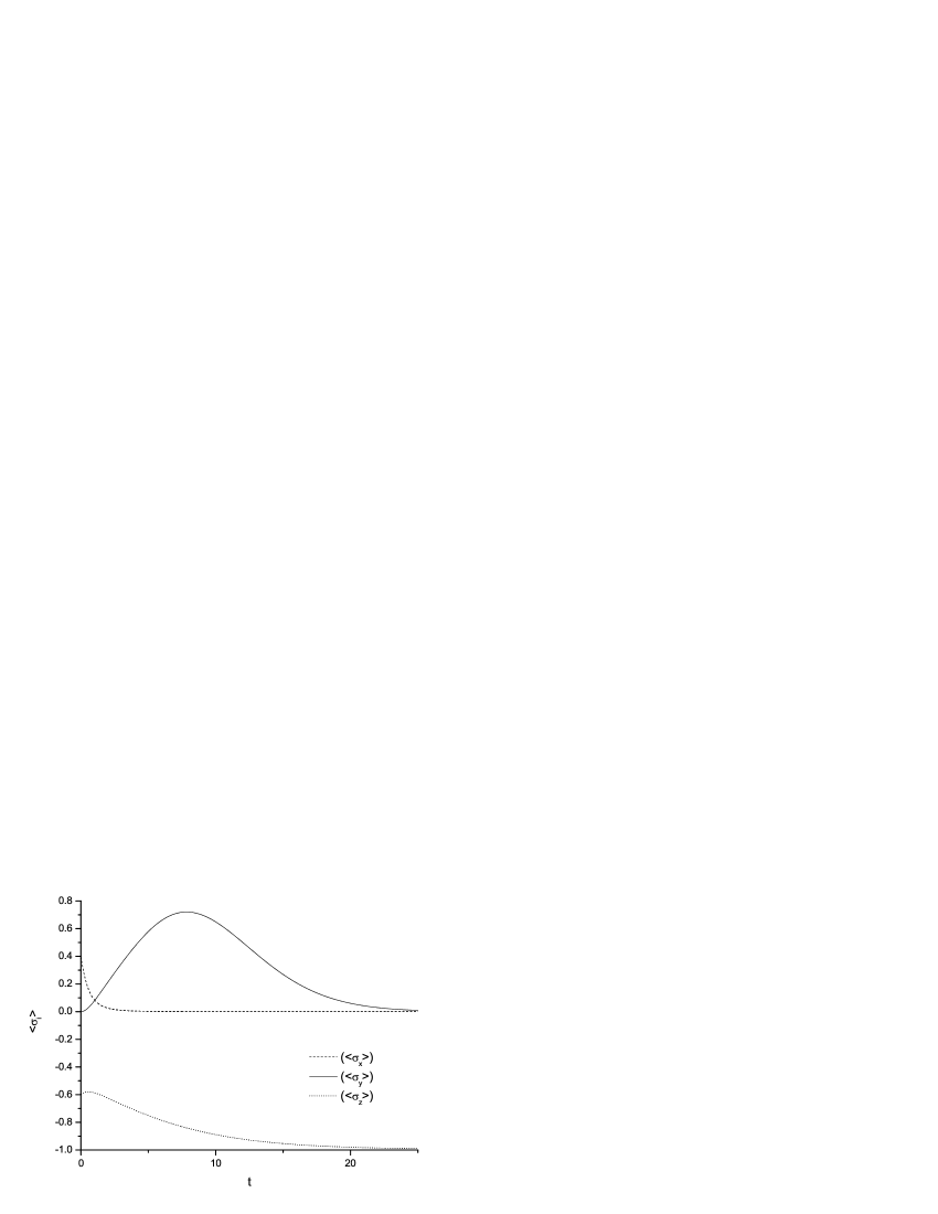
Figure 6: The time-dependence of $\langle\sigma_{i}\rangle$ with parameters $r=0.6e^{-0.1t}$, $\mu=\sqrt{0.2}$, and $\nu=\sqrt{0.8}$.

References

• (1) J. Plebański, Phys. Rev. 101, 1825 (1956).
• (2) H.P. Yuen, Phys. Rev. A 13, 2226 (1976).
• (3) R.E. Slusher, W. Hollberg, B. Yurke, J.C. Mertz, and J.F. Valley, Phys. Rev. Lett. 55, 2409 (1985).
• (4) E.S. Polzik, J. Carri and H.J. Kimble, Phys. Rev. Lett. 68, 3020 (1992).
• (5) A. Furusawa et al., Science 282, 706 (1998).
• (6) H.A. Haus, Electromagnetic Noise and Quantum Optical Measurements (Spinger-verlag, Berlin, 2000).
• (7) M.O. Scully and M.S. Zubairy, Quantum Optics (Cambridge UP, London, 1997).
• (8) C.W. Gardiner and P. Zoller, Quantum Noise (Spinger-verlag, New York, Sec. edition, 2000).
• (9) D.F. Walls and G.J. Milburn, Quantum Optics (Spinger-verlag, New York, Berlin, 1994).
• (10) C. Anastopoulos and B. L. Hu, Phys. Rev. A 62, 033821 (2000).
• (11) S.J. Wang, D. Zhao, H. G. Luo, L. X. Cen, and C. L. Jia, Phys. Rev. A 64, 052102 (2001).
• (12) S. J. Wang, M. C. Nemes, A. N. Salgueiro, and H. A. Weidenmueller, Phys. Rev. A 66, 033608(2002).
• (13) S.J. Wang, J.H. An, H.G. Luo and C.L. Jia, J. Phys. A: Math. Gen. 36, 829 (2003).
• (14) S.J. Wang, F.L. Li and Weiguny, Phys. Lett. A 180, 189 (1993).
• (15) Shun-jin Wang, Jian-min Cao and A. Weiguny, Phys. Rev. A 40, 1225 (1989).
• (16) C.W. Gardiner, Phys. Rev. Lett. 56, 1917 (1986).
• (17) B.J. Dalton, Z. Ficek and S. Swain, J. of Mod. Optics 46, 379 (1999).
• (18) P. Mores and H. Feshbach, Methods of Theoretical Physics (New York: Wiley, 1980).
• (19) H.-J. Briegel and B.-G. Englert, Phys. Rev. A 47, 3311 (1993).
• (20) M. Jakob and S. Stenholm, Phys. Rev. A 69, 042105 (2004).
• (21) M. Jakob and S. Stenholm, Phys. Rev. A 70, 012104(2004).
• (22) K. Bergmann, H. Theuer, and B.W. Shore, Rev. Mod. Phys. 70, 1003 (1998).
Refer to caption