Abstract

The vast majority of the literature dealing with quantum dynamics is concerned with linear evolution of the wave function or the density matrix. A complete dynamical description requires a full understanding of the evolution of measured quantum systems, necessary to explain actual experimental results. The dynamics of such systems is intrinsically nonlinear even at the level of distribution functions, both classically as well as quantum mechanically. Aside from being physically more complete, this treatment reveals the existence of dynamical regimes, such as chaos, that have no counterpart in the linear case. Here, we present a short introductory review of some of these aspects, with a few illustrative results and examples.

Nonlinear Quantum Dynamics

1 Introduction

It is hard to imagine a scientific discipline older than the study of dynamical systems. The remarkable history of the field testifies to nature’s inexhaustible store of subtlety and ability to surprise. Ever since Galileo, remarkable experiments, deep theoretical insights, and powerful calculational tools have all contributed to creating the rich panorama that the field presents today.

From a theoretical perspective, dynamical systems are specified by the rules of evolution and the physical objects to which these rules apply. Our fundamental notions regarding both aspects have undergone radical changes in the past few hundred years. Classical mechanics has made way for quantum mechanics and absolute notions of space and time have been replaced by the unified viewpoint of classical general relativity. A key lesson to be drawn from these advances is that even the most basic notions regarding the nature of physical information must change as our overall understanding progresses.

The next step forward has yet to be taken: The clash between relativity and quantum mechanics – the choice between causality and unitarity – awaits resolution. However, on a less grand scale, the tension between fundamentally different points of view is already apparent in the discord between quantum and classical mechanics. Unlike special relativity, where $v/c\rightarrow 0$ smoothly transitions between Einstein and Newton, the limit $\hbar\rightarrow 0$ is singular. The symmetries underlying quantum and classical dynamics – unitarity and symplecticity, respectively – are fundamentally incompatible with the opposing theory’s notion of a physical state: quantum-mechanically, a positive semidefinite density matrix; classically, a positive phase-space distribution function.

Chaos provides an excellent illustration of this dichotomy of world-views [1]. Without question, chaos exists, can be experimentally probed, and is well-described by classical mechanics. But the classical picture does not simply translate to the quantum view; attempts to find chaos in the Schrodinger equation for the wave function, or, more generally, the quantum Liouville equation for the density matrix, have all failed. This failure is due not only to the linearity of the equations, but also the Hilbert space structure of quantum mechanics which, via the uncertainty principle, forbids the formation of fine-scale structure in phase space, and thus precludes chaos in the sense of classical trajectories. Consequently, some people have even wondered if quantum mechanics fundamentally cannot describe the (macroscopic) real world.

It is therefore clear that there is more than sufficient motivation for investigating the notion of nonlinearity in classical and quantum theories. The main point of this article is to provide an angle of vision which sets nonlinearity in its experimentally relevant context. Familiar to control theorists [2] – but much less so to most physicists – this perspective bridges the classical and quantum points of view and smoothly connects them with each other.

The article is organized as follows. We will begin with a discussion of the various possibilities of dynamical description, clarify what is meant by “nonlinear quantum dynamics,” discuss its connection to nonlinear classical dynamics, and then study two experimentally relevant examples of quantum nonlinearity – (i) the existence of chaos in quantum dynamical systems far from the classical regime, and (ii) real-time quantum feedback control.

The results described here are due to the efforts of many people spread over the last thirty years or so, some results being even older. Unfortunately, space limitations prevent anywhere near an adequate job of referencing, for which a sympathetic understanding is begged in advance. Restrictions also meant the omission of important topics and explanations of derivations.

2 Evolution: Isolated, Open, and Conditioned

How should one describe a dynamical system? Before settling on a definition, it is best to first ask some important physical questions. As an illustrative example, a situation worth learning from arose in the attempt to define a field-theoretic notion of a particle in a general spacetime [3]. In Minkowski space, the formal definition is simple: positive energy plane-waves, but this definition cannot be extended to arbitrary metrics. It soon became clear that the correct way to approach the problem was to give up the attempt to arrive at a formal definition and replace it with a physical definition: “A particle is what a particle detector detects.” Thus, specifying a field theory Lagrangian is not sufficient to define the notion of a particle, additionally we must model the detector and how it couples to the field. Just what a physical “particle” is depends on the design of the detector and the field-detector coupling.

Keeping the lesson of the above example in mind, we will explore three different dynamical possibilities below: isolated evolution, where the system evolves without any coupling to the external world, unconditioned open evolution, where the system evolves coupled to an external environment but where no information regarding the system is extracted from the environment, and conditioned open evolution where such information is extracted. In the third case, the evolution of the physical state is driven by the system evolution, the coupling to the external world, and by the fact that observational information regarding the state has been obtained. This last aspect – system evolution conditioned on the measurement results via Bayesian inference – leads to an intrinsically nonlinear evolution for the system state. The conditioned evolution provides, in principle, the most realistic possible description of an experiment. To the extent that quantum and classical mechanics are eventually just methodological tools to explain and predict the results of experiments, this is the proper context in which to compare them.

2.1 Isolated and Open Evolution

Suppose we are given an arbitrary system Hamiltonian $H(x,p)$ in terms of the dynamical variables $x$ and $p$; we will be more specific regarding the precise meaning of $x$ and $p$ later. The Hamiltonian is the generator of time evolution for the physical system state, provided there is no coupling to an environment or measurement device. In the classical case, we specify the initial state by a positive phase space distribution function $f_{Cl}(x,p)$; in the quantum case, by the (position-representation) positive semidefinite density matrix $\rho(x_{1},x_{2})$ or, completely equivalently, by the Wigner distribution function $f_{W}(x,p)$ [4] (not positive).

The evolution of an isolated system is then given by the classical and quantum Liouville equations for the fine-grained distribution functions (i.e., the evolution is entropy-preserving):

$$\partial_{t}f_{Cl}(x,p) = -\left[\frac{p}{m}\partial_{x}-\partial_{x}V(x)\partial_{p}\right]f_{Cl}(x,p),$$ (1)

$$\partial_{t}f_{W}(x,p) = -\left[\frac{p}{m}\partial_{x}-\partial_{x}V(x)\partial_{p}\right]f_{W}(x,p)$$ (2)

$$+\sum_{\lambda=1}^{\infty}\frac{(\hbar/2i)^{2\lambda}}{(2\lambda+1)!}\partial_{x}^{2\lambda+1}V(x)\partial_{p}^{2\lambda+1}f_{W}(x,p),$$

here we have assumed for simplicity that the potential $V(x)$ can be Taylor-expanded. Note that these evolutions are both linear in the respective distribution functions. Classically, the limit $f_{Cl}(x,p)=\delta(x-\bar{x})\delta(p-\bar{p})$ is allowed, and, on substitution in Eqn. (2), yields Newton’s equations. These may then be interpreted as equations for the particle position and momentum, although this identification is only formal at this stage (as in the Minkowski space definition of a particle in the field theory example). Quantum mechanically, this ultralocal limit is not allowed as $f_{W}(x,p)$ must be square-integrable, therefore, even formally, no direct particle interpretation exists (an obstacle that arises as something new is added – just like the difficulty with generalizing the notion of a particle to arbitrary metrics discussed above).

The basic idea behind extension to open systems is simple to state but not easy to implement in practice. The complete Hamiltonian now includes a piece representing the environment and another, the system-environment coupling. If the environment is in principle unobservable, then a (nonlocal in time) linear master equation for the system’s reduced density matrix is derivable by tracing over the environmental variables (in practice, tractable equations are impossible to obtain without drastic simplifying assumptions such as weak coupling, timescale separations, and simple forms for the environmental and coupling Hamiltonians). In any case, the important point to note is that the act of tracing over the environment does not change the linear nature of the equations. Generally speaking, master equations describing open evolution of coarse-grained distributions augment the RHS of Eqns. (2) and (2) with terms containing dissipation and diffusion kernels connected via generalized fluctuation-dissipation relations [5]. While the classical diffusion term vanishes in the limit of zero temperature for the environment, this is not true quantum mechanically due to the presence of zero-point fluctuations.

2.2 Conditioned Evolution

Conditioned evolution of the type we are interested in here is fundamentally different from the equations discussed above. We assume that measurements are possible on the environment and ask what the evolution of the reduced density matrix of the system is, given that the results of these measurements are known [6]. Let us consider an example. Suppose we wish to measure the position of a nanomechanical oscillator (Fig. 1). By electrostatically coupling the resonator to a single-electron transistor (SET), and measuring the (classical) SET current – the measurement record – we are in fact measuring the transverse displacement of the resonator. In this situation, the evolution of the reduced density matrix of the system must contain a term that reflects the gain in information arising from the measurement record (“innovation” in the language of control theory). This term, arising from applying a continuous analog of Bayes’ theorem, is intrinsically nonlinear in the distribution function. The coupling to an external probe (and the associated environment) will also cause effects very similar to the open evolution considered earlier, and there can once again be dissipation and diffusion terms in the evolution equations. The primary differences between the classical and quantum treatments, aside from the kinematic constraints on the distribution functions, are the following: (i) the (nonlocal in $p$) quantum evolution term in Eqn. (2), and (ii) an irreducible diffusion contribution due to quantum backaction reflecting the active nature of quantum measurements.

Figure 1: A nanomechanical resonator: the thin central bar is coated with a conductor (gold) which also forms the T-shaped control electrode to the left. The thin line parallel to the resonator is the central island of a single-electron transistor which serves as the position sensor.

We now consider a simple model of position measurement to provide a measure of concreteness. In this model, we will assume that there are no environmental channels aside from those associated with the measurement. Suppose we have a single quantum degree of freedom, position in this case, under a weak, ideal continuous measurement [7]. Here “ideal” refers to no loss of information during the measurement, i.e., a fine-grained evolution with no change in entropy. Then, we have two coupled equations, one for the measurement record $y(t)$,

$$dy=\langle x\rangle dt+dW/{\sqrt{8k}}$$ (3)

where $dy$ is the infinitesimal change in the output of the measurement device in time $dt$, the parameter $k$ characterizes the rate at which the measurement extracts information about the observable, i.e., the strength of the measurement [8], and $dW$ is the Wiener increment describing driving by Gaussian white noise [9], the difference between the observed value and that expected. The other equation – the nonlinear stochastic master equation (SME) – specifies the resulting conditioned evolution of the system density matrix, given below in the Wigner representation,

$$f_{W}(x,p,t+dt) = \left[1+dt\left[-\frac{p}{m}\partial_{x}+\partial_{x}V(x)\partial_{p}+D_{BA}\partial_{p}^{2}\right]\right.$$ (4)

$$+\left.dt\sum_{\lambda=1}^{\infty}\!\frac{\left(\hbar/2i\right)^{2\lambda}}{(2\lambda+1)!}\partial_{x}^{2\lambda+1}V(x,t)\partial_{p}^{2\lambda+1}\right]f_{W}(x,p,t)$$

$$+dt\sqrt{8k}(x-\langle x\rangle)f_{W}(x,p,t)dW,$$

where $D_{BA}=\hbar^{2}k$ is the diffusion coefficient arising from quantum backaction and the last (nonlinear) term represents the conditioning due to the measurement. In principle, there is also a (generalized) damping term [10], but if the measurement coupling is weak enough, it can be neglected. If we choose to average over all the measurement results, which is the same as ignoring them, then the conditioning term vanishes, but not the diffusion from the measurement backaction. Thus the resulting linear evolution of the coarse-grained quantum distribution is not the same as the linear fine-grained evolution (2), but yields a conventional open-system master equation. Moreover, for a given (coarse-grained) master equation, different underlying fine-grained SME’s may exist, specifying different measurement possibilities.

The classical conditioned master equation [set $\hbar=0$ in Eqn. (4), holding $k$ fixed],

$$f_{Cl}(x,p,t+dt) = \left[1-dt\left[\frac{p}{m}\partial_{x}-\partial_{x}V(x)\partial_{p}\right]\right]f_{Cl}(x,p,t)$$ (5)

$$+dt\sqrt{8k}(x-\langle x\rangle)f_{Cl}(x,p,t)dW,$$

does not have the backaction term as classical measurements are passive: Averaging over all measurements simply gives back the Liouville equation (2), and there is no difference between the fine-grained and coarse-grained evolutions in this special case. [In general, classical diffusion terms from ordinary open evolution can also co-exist, as in the more general a posteriori evolution specified by the Kushner-Stratonovich equation [11].] As a final point, we will delay our discussion of how the classical trajectory limit is incorporated in Eqn. (5), i.e., the precise sense in which the “the position of a particle is what a position-detector detects” to the next section.

3 QCT: The Quantum-Classical Transition

As mentioned already, quantum and classical mechanics are fundamentally incompatible in many ways, yet the macroscopic world is well-described by classical dynamics. Physicists have struggled with this quandary ever since the laying of the foundations of quantum theory. It is fair to say that, even today, not everyone is satisfied with the state of affairs – including many seasoned practitioners of quantum mechanics.

If quantum mechanics is really the fundamental theory of our world, then an effectively classical description of macroscopic systems must emerge from it – the so-called quantum-classical transition (QCT). It turns out that this issue is inextricably connected with the question of the physical meaning of dynamical nonlinearity discussed in the Introduction. The central thesis is that real experimental systems are by definition not isolated, hence the QCT must be viewed in the relevant physical context.

Quantum mechanics is intrinsically probabilistic, but classical theory – as shown above by the existence of the delta-function limit for the classical distribution function – is not. Since Newton’s equations provide an excellent description of observed classical systems, including chaotic systems, it is crucial to establish how such a localized description can arise quantum mechanically. We will call this the strong form of the QCT. Of course, in many situations, only a statistical description is possible even classically, and here we will demand only the agreement of quantum and classical distributions and the associated dynamical averages. This defines the weak form of the QCT.

3.1 The Strong Form of the QCT

It is clear that the strong form of the QCT is impossible to obtain from either the isolated or open evolution equations for the density matrix or Wigner function. For a generic dynamical system, a localized initial distribution tends to distribute itself over phase space and either continue to evolve in complicated ways (isolated system) or asymptote to an equilibrium state (open system) – whether classically or quantum mechanically. In the case of conditioned evolution, however, the distribution can be localized due to the information gained from the measurement. In order to quantify how this happens, let us first apply a cumulant expansion to the (fine-grained) conditioned classical evolution (5), resulting in the equations for the centroids ($\bar{x}\equiv\langle x\rangle$, $\bar{p}\equiv\langle p\rangle$),

$$d\bar{x}=\frac{\bar{p}}{m}dt+\sqrt{8k}C_{xx}dW,~{}~{}~{}d\bar{p}=\langle F(x)\rangle dt+\sqrt{8k}C_{xp}dW,$$ (6)

where

$$F(x)=-\partial_{x}V(x),~{}~{}~{}C_{AB}=(\langle AB\rangle+\langle BA\rangle-2\langle A\rangle\langle B\rangle)/2,$$ (7)

along with a hierarchy of coupled equations for the time-evolution of the higher cumulants. These equations are the continuous measurement, real-world, analog of the formal ultralocal Newtonian limit of the distribution function in the classical Liouville equation (2). While Eqns. (6) always apply, our aim is to determine the conditions under which the cumulant expansion effectively truncates and brings their solution very close to that of Newton’s equations. This will be true provided the noise terms are small (in an average sense) and the force term is localized, i.e., $\langle F(x)\rangle=F(\bar{x})+\cdots$, the corrections being small. The required analysis involves higher cumulants and has been carried out in Ref. [12]. (Ref. [12] also points to previous literature.) It turns out that the distribution will be localized provided

$$8k\gg\sqrt{\frac{(\partial_{x}^{2}F)^{2}|\partial_{x}F|}{2mF^{2}}}$$ (8)

and the motion of the centroid will effectively define a smooth classical trajectory – the low-noise condition – as long as

$$k\gg\frac{2|\partial_{x}F|}{S}$$ (9)

where $S$ is the action scale of the system. Note that this condition does not bound the measurement strength.

We now turn to the quantum version of these results. In this case, the analogous cumulant expansion gives exactly the same equations for the centroids as above, while the equations for the higher cumulants are different. We can again investigate whether a trajectory limit exists. Localization holds in the weakly nonlinear case if the classical condition above is satisfied. In the case of strong nonlinearity, the inequality becomes

$$8k\gg\frac{(\partial_{x}^{2}F)^{2}\hbar}{4mF^{2}}.$$ (10)

Because of the backaction, the low-noise condition is implemented in the quantum case by a double-sided inequality:

$$\frac{2|\partial_{x}F|}{s}\ll\hbar k\ll\frac{|\partial_{x}F|s}{4},$$ (11)

where the action is measured in units of $\hbar$, $s$ being dimensionless. The left inequality is the same as the classical one discussed above, however the right inequality is essentially quantum mechanical. The measurement strength cannot be made arbitrarily large as the backaction will result in too large a noise in the equations for the centroids. As the action $s$ is made larger, both inequalities are satisfied for an ever wider range of $k$. For continuously measured quantum systems, trajectories that emerge in the macroscopic limit follow Newton’s equations, and hence can be chaotic as shown in Ref. [12]. Thus, as speculated in a prescient paper by Chirikov [13], measurement indeed provides the missing link between “quantum” and “chaos.”

3.2 The Weak Form of the QCT

If the conditions enforcing the strong form of the QCT are satisfied, then the weak form follows automatically. The reverse is not true, however: results from a coarse-grained analysis cannot be applied to the fine-grained situation. Moreover, the violation of the strong inequalities (11) need not prevent a weak QCT: It does not matter if the distribution is too wide, as long as the classical and quantum distributions agree, and, even if the backaction noise is large, the coarse-grained distribution remains smooth and the weak quantum-classical correspondence can still exist. Consequently, the weak form of the QCT has to be approached in a different manner. In fact, the weak version is just another way to state the conventional decoherence idea; however, as discussed elsewhere [14], mere suppression of quantum interference does not guarantee the QCT even in the weak form.

In a recent analysis carried out for a bounded open system with a classically chaotic Hamiltonian, it has been argued that the weak form of the QCT is achieved by two parallel processes [15], explaining earlier numerical results [16]. First, the semiclassical approximation for quantum dynamics, which breaks down for classically chaotic systems due to overwhelming nonlocal interference, is recovered as the environmental interaction filters these effects. Second, the environmental noise restricts the foliation of the unstable manifold (the set of points which approach a hyperbolic point in reverse time) allowing the semiclassical wavefunction to track this modified classical geometry.

It turns out that this analysis applies only to systems with a bounded phase space. It is possible that topological restrictions on the accessible phase space – and not only the form of the particular Hamiltonian – play a crucial role in determining when the weak form of the QCT actually applies. For example, this might explain why the open-system quantum delta-kicked rotor is a counter-example to naive expectations regarding the QCT [14].

4 Chaos and Quantum Mechanics

The results of the previous section have already established that classical chaos and quantum mechanics are not incompatible in the macroscopic limit. The question then naturally arises whether observed quantum mechanical systems can be chaotic far from the classical limit? This question is particularly significant as closed quantum mechanical systems are not chaotic, at least in the conventional sense of dynamical systems theory [17]. In the case of observed systems it has recently been shown, by defining and computing a maximal Lyapunov exponent applicable to quantum trajectories, that the answer is in the affirmative [18]. Thus, realistic quantum dynamical systems are chaotic in the conventional sense and there is no fundamental conflict between quantum mechanics and the existence of dynamical chaos.

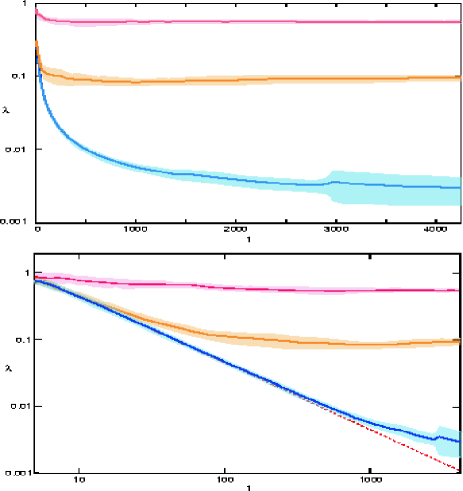
Figure 2: Finite-time Lyapunov exponents $\lambda(t)$ for a driven Duffing oscillator with measurement strengths $k=5\times 10^{-4},~{}0.01,~{}10$, averaged over 32 trajectories (linear scale in time, top, and logarithmic scale, bottom; bands indicate the standard deviation over the 32 trajectories) [18]. The (analytic) $1/t$ fall-off at small $k$ values (dashed red line), prior to the asymptotic regime, is evident in the bottom panel.

The basic idea in Ref. [18] is to focus attention on a single time-series, say, the expectation value $\langle x\rangle$, and analyze it for chaos. Following Ref. [18] the Lyapunov exponent is defined to be

$$\lambda=\lim_{t\rightarrow\infty}\lim_{\Delta_{s}(0)\rightarrow 0}\frac{1}{t}\ln\Delta_{s}(t)\equiv\lim_{t\rightarrow\infty}\lambda_{s}(t)$$ (12)

where the subscript $s$ denotes the particular noise realization and $\Delta(t)=|\langle x(t)\rangle-\langle x_{fid}(t)\rangle|$ defines the divergence between two “trajectories.” The noise realization is kept fixed when calculating $\Delta(t)$. For isolated systems it is possible to prove that the Lyapunov exponent is zero, with the finite-time exponent vanishing as $1/t$, as $t\rightarrow\infty$ [18]. This is consistent with our expectation of not finding chaos for linear evolution. In the case of conditioned nonlinear evolution, however, the situation can be dramatically different as shown in Fig. 2. What we find is that for small $k$, $\lambda(t)$ first falls as $1/t$ (as for $k=0$), but then stabilizes at an asymptotic value which is $k$-dependent, and different from the classical value. Even at values of $k$ small enough that the strong inequalities (11) are not satisfied, $\lambda$ is finite, and the evolution is, thus, chaotic.

We stress that the chaos identified here is not merely a formal result - even deep in the quantum regime, the Lyapunov exponent can be obtained from measurements on a real system. Quantum predictions of this type can be tested in the near future, e.g., in cavity QED and nanomechanics experiments [19]. Experimentally, one would use the known measurement record to integrate the SME; this provides the time evolution of the mean value of the position. From this fiducial trajectory, given the knowledge of the system Hamiltonian, the Lyapunov exponent can be obtained by following the procedure described above. It is important to keep in mind that these results form only a starting point for the further study of nonlinear quantum dynamics and its theoretical and experimental ramifications.

5 Quantum Feedback Control

To illustrate an application of nonlinear quantum dynamics, we now consider real-time control of quantum dynamical systems. Feedback control is essential for the operation of complex engineered systems, such as aircraft and industrial plants. As active manipulation and engineering of quantum systems becomes routine, quantum feedback control is expected to play a key role in applications such as precision measurement and quantum information processing. The primary difference between the quantum and classical situations, aside from dynamical differences, is the active nature of quantum measurements. As an example, in classical theory the more information one extracts from a system, the better one is potentially able to control it, but, due to backaction, this no longer holds true quantum mechanically.

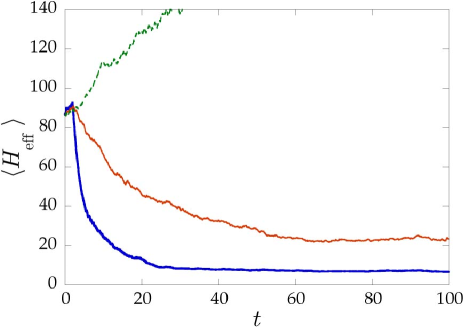
Figure 3: Feedback cooling in cavity QED: Evolution of the mean atomic effective energy, with no cooling (top curve), cooling based on direct feedback of the photocurrent signal (middle), cooling based on feedback with a simple Gaussian state estimator (bottom). Note the improved cooling efficiency in the second case.

Controlling quantum systems is possible using state-estimation ideas as pioneered by Belavkin [20] or direct feedback of the measured classical current [21]. Applications studied so far include controlling atomic [22] and qubit [23] states as well as active cooling of dynamical degrees of freedom. As one example, let us consider an atom trapped in a high-finesse optical cavity in the strong-coupling limit, with the output laser light monitored via homodyne detection. The resulting photocurrent provides information about the position of the atom in the cavity which, in turn, can be used to cool the atom’s position degree of freedom by varying the intensity of the driving laser field [24] (Fig. 3). Nanomechanical resonators can also be cooled by feedback. Here, the present state of the art has reached the point where the resonators are less than a factor of 10 away from the quantum limit, i.e., the point where the thermal energy is less than the energy of the resonator ground state. Lowering the temperature of the resonators to the mK regime would allow this goal to be reached. In principle, active cooling could achieve this by measuring the resonator position using a SET as described earlier (Fig. 1) and then applying (damping) feedback through the control electrode [25]. Experiments to test this idea are currently in progress.

1

References

- [1] See, e.g., A. Peres, Quantum Theory: Concepts and Methods (Kluwer, 1993).
- [2] P.S. Maybeck, Stochastic Models, Estimation and Control (Academic Press, New York, 1982); O.L.R. Jacobs, Introduction to Control Theory (Oxford University Press, Oxford, 1993).
- [3] W.G. Unruh, Phys. Rev. D 14, 870 (1976).
- [4] For reviews, see M. Hillery, R. O’Connell, M.O. Scully, and E.P. Wigner, Phys. Rep. 106, 121 (1984); V.I. Tatarskii, Usp. Fiz. Nauk 139, 587 (1983).
- [5] L.P. Kadanoff and G. Baym, Quantum Statistical Mechanics (Addison-Wesley, Redwood City, 1989); R. Zwanzig, Nonequilibrium Statistical Mechanics (Oxford University Press, New York, 2001); K. Blum, Density Matrix Theory and Applications (Plenum Press, New York, 1996).
- [6] For textbook treatments, see H.J. Carmichael, An Open Systems Approach to Quantum Optics (Springer, 1993); C.W. Gardiner and P. Zoller, Quantum Noise (Springer, 2000); M. Orszag, Quantum Optics (Springer, 2000).
- [7] C.M. Caves and G.J. Milburn, Phys. Rev. A 36, 5543 (1987); G.J. Milburn, Quantum Semiclass. Opt. 8, 269 (1996); A.C. Doherty and K. Jacobs, Phys. Rev. A 60, 2700 (1999); P. Warszawski and H.M. Wiseman, J. Opt. B 5, 1 (2003).
- [8] A.C. Doherty, K. Jacobs, and G. Jungman, Phys. Rev. A 63, 062306 (2001).
- [9] D.T. Gillespie, Am. J. Phys. 64, 225 (1996).
- [10] See, e.g., D. Mozyrsky and I. Martin, Phys. Rev. Lett. 89, 018301 (2002).
- [11] T.P. McGarty, Stochastic Systems and State Estimation (Wiley-Interscience, New York, 1974).
- [12] T. Bhattacharya, S. Habib, and K. Jacobs, Phys. Rev. Lett. 85, 4852 (2000); Phys. Rev. A 67, 042103 (2003).
- [13] B.V. Chirikov, Chaos 1, 95 (1991).
- [14] S. Habib, K. Jacobs, H. Mabuchi, R. Ryne, K. Shizume, and B. Sundaram, Phys. Rev. Lett. 88, 040402 (2002).
- [15] B. Greenbaum, S. Habib, K. Shizume, and B. Sundaram, quant-ph/0401174.
- [16] S. Habib, K. Shizume, and W.H. Zurek, Phys. Rev. Lett. 80, 4361 (1998).
- [17] R. Kosloff and S.A. Rice, J. Chem. Phys. 74, 1340 (1981); J. Manz, J. Chem. Phys. 91, 2190 (1989).
- [18] S. Habib, K. Jacobs, and K. Shizume, quant-ph/0412159; and in preparation.
- [19] H. Mabuchi and A.C. Doherty, Science 298, 1372 (2002); M.D. LaHaye, O. Buu, B. Camarota, and K.C. Schwab, Science 304, 74 (2004).
- [20] V.P. Belavkin, Comm. Math. Phys. 146, 611 (1992); V.P. Belavkin, Rep. Math. Phys. 43, 405 (199); A.C. Doherty, S. Habib, K. Jacobs, H. Mabuchi, and S.-M. Tan, Phys. Rev. A 62, 012105 (2000).
- [21] H.M. Wiseman and G.J. Milburn, Phys. Rev. Lett. 70, 548 (1993).
- [22] H.M. Wiseman, S. Mancini, and J. Wang, Phys. Rev. A 66, 013807 (2002).
- [23] R. Ruskov and A.N. Korotkov, Phys. Rev. B 66, 041401(R) (2002).
- [24] D.A. Steck, K. Jacobs, H. Mabuchi, T. Bhattacharya, and S. Habib, Phys. Rev. Lett. 92, 223004 (2004).
- [25] A. Hopkins, K. Jacobs, S. Habib, and K. Schwab, Phys. Rev. B 68, 235328 (2003).