SPECTRAL APPROACH TO CHAOS AND QUANTUM-CLASSICAL CORRESPONDENCE IN QUANTUM MAPS

Abstract

Correspondence in quantum chaotic systems is lost in short time scales. Introducing some noise we study the spectrum of the resulting coarse grained propagaor of density matrices. Some differen methods to compute the spectrum are reviewed. Moreover, the relationship between the eigenvalues of the coarse-grained superoperator and the classical Ruelle-Pollicott resonances is remarked. As a concequence, classical decay rates in quantum time dependent quantities appear.

I Introduction

Since the beginings of quantum theory, the problem of the transition from the quantum to the classical world has posed interesting and challenging questions. The concept of decoherencezurekRMP has introduced some clarity, yet many questions remain to be answered.

Quantum chaos studies the emergence of classical chaotic behavior in quantum systems as $\hbar\to 0$. The introduction of Gutzwiller’s trace formulagutz and the developement of periodic orbit theorieschaosbook ; vergini ; heller and in addition the understanding of the influence of random matrix theoriesbohigas gave quantum chaos a boost of interest. One key feature of quantum chaotic systems is that correspondence is lost in very short time scales (Eherenfest timeberman ). The introduction of noise (in a controlled way) restores correspondence and allows to study it from the point of view of the appearance of classical properties from the quantum systems. In this way, the classical Lyapunov exponent plays an important role in the medium time decay of time dependent quantitites like the linear entropybianucci ; garma and the Loschmidt echojalabert ; losch .

The study of this correspondence for long times, like for example the asymptotic behavior of correlation functions, requires the understanding of the spectral properties of both quantum and classical propagators and their relationship in the $\hbar\to 0$ limit.

In this review the latter approach is discussed in detail although the former is also addressed. Some recent techniques to compute the spectrum of both the classical and the quantum propagator of densities are described. We describe in detail some efficient methods used by the authors recentlygarma ; garma2 ; aolita . The systems are quantum maps on the torus. By introducing diffusion in the form of Gaussian noise we obtain a coarse grained quantum propagatornonn . The Gaussian noise introduces a natural truncation that is understood using phase space representation theory (chord funtion and Wigner function). In addition, we develop an iteration method that efficiently provides the leading part of the spectrum. Relation to the classical Ruelle-Pollicott resonances is then established by taking the limit $\hbar\to 0$ and also by studying the long time decay rates of several quantities.

This review is organized as follows. In Sec. II we define the phase space we will work with and summarize some operator theoretic properties of representations in phase space. A brief introduction to the theory of Open Quantum systems is provided in Sec. III. In sections IV and V quantum maps and the model used for open quantum maps are described. The kind of Gaussian noise used, in term of phase space translations and how it acts when composed with a unitary superoperator, yielding a coarse grained propagator, is developed in Sec. VI while the issue of correspondence, specifically through the relations between classical and quantum spectrum is addressed in Sec. VII. Finally in Sec. VIII, some numerical methods to compute the spectrum are described. The consequences for the asymptotic decay for long times are discussed in Sec. VIII.4.

II Phase space

II.1 Torus quantization

All the calculations are made for systems with a bounded phase space, which for simplicity we take to be a 2-Torus ($\mathbb{T}^{2}$).

There are some well-known features that appear in the quantization of $\mathbb{T}^{2}$. Since the area is finite, and normalized to unity, the Hilbert ${\cal H}_{N}$ space is finite and of dimension $N$. The value of $N$ determines an effective Planck constant

$$\hbar=\frac{1}{2\pi N}.$$ (1)

The position and momentum bases are discrete sets

$$\begin{array}[]{c}{\cal B}_{q}=\{|q_{i}\rangle,q_{i}=0,1,\ldots N-1\}\\ {\cal B}_{p}=\{|p_{j}\rangle,p_{j}=0,1,\ldots N-1\}\end{array},$$ (2)

which define an $N\times N$ grid $G_{N}$. We identify with $|q_{i}\rangle$ the position $q_{i}/N$ and with $|p_{j}\rangle$ the momentum $p_{j}/N$. They are related by the discrete Fourier transform (DFT) of dimension $N$,

$$\langle p|q\rangle=\frac{1}{\sqrt{N}}\,e^{-(2\pi{\rm i}/N)qp}.$$ (3)

Pure states are represented by $N$-dimensional vectors $|\phi\rangle$ in ${\cal H}_{N}$. Mixed states are best described by the density operator $\hat{\rho}$. If we identify Liouville space ${\cal H}_{N^{2}}$ with the space of comlplex $N\times N$ matrices, then density operators associated to states in ${\cal H}_{N}$ form a subset of ${\cal H}_{N^{2}}$ of self-adjoint, positive semidefinite matrices, with unit trace. Moreover

$$\mbox{Tr}(\hat{\rho}^{2})\leq 1,$$ (4)

with the equality holding iff the state is pure.

We now define the translation operators on $\mathbb{T}^{2}$. In $\mathbb{R}^{2}$ the Weyl group defines the translation operator of $q_{1}$ in position and $p_{1}$ in momentum, as

$$\hat{T}_{(q,p)}=e^{-({\rm i}/\hbar)(q_{1}\hat{P}-p_{1}\hat{Q})}.$$ (5)

Translations on the torus are somewhat harder to define because infinitesimal operators $\hat{Q}$ and $\hat{P}$ with the canonical commutation rules cannot be defined in a discrete Hilbert space. Nevertheless, finite cyclic shifts $\hat{U}$ and $\hat{V}$ such that, if $|q\rangle$ and $|p\rangle$ are position and momentum eigenstates respectively, can be definedschwinger as

$$\begin{array}[]{ccccccr}\hat{U}^{q_{1}}|q\rangle&=&|q+q_{1}\rangle;&&\hat{U}^{q_{1}}|p\rangle&=&e^{-(2\pi{\rm i}/N)q_{1}p}|p\rangle;\\ \hat{V}^{p_{1}}|p\rangle&=&|p+p_{1}\rangle;&&\hat{V}^{p_{1}}|q\rangle&=&e^{(2\pi{\rm i}/N)p_{1}q}|q\rangle\end{array}.$$ (6)

These operators satisfy the comutation rule

$$\hat{V}^{p}\hat{U}^{q}=\hat{U}^{q}\hat{V}^{p}e^{(2\pi{\rm i}/N)qp}.$$ (7)

Symmetrizing Eq. (7) one gets the transaltion operators on the quantized torus as a composition of position and momentum shifts,

$$\hat{T}_{(q,p)} = \hat{U}^{q}\hat{V}^{p}e^{({\rm i}\pi/N)qp}$$ (8)

$$= \hat{V}^{p}\hat{U}^{q}e^{-({\rm i}\pi/N)qp}$$

with $q,p=0,\ldots,N-1$. There are $N^{2}$ operators $\hat{T}_{(q,p)}$ and have the following property

$$\mbox{Tr}(\hat{T}_{\alpha}^{\dagger}\hat{T}_{\beta})=N\delta_{\alpha\beta},$$ (9)

for all $\alpha,\beta$ (when convenient we use greek letters to rperesent a phase space point, e. g. $\alpha\equiv(q,p)$). Therefore, they constitute a complete orthogonal set in the Hilbert-Schmidt inner product. Moreover, they have the group composition rule

$$\hat{T}_{\alpha}\hat{T}_{\beta}=e^{({\rm i}\pi/N)\alpha\wedge\beta}\hat{T}_{\alpha+\beta}$$ (10)

where $\alpha\wedge\beta$ is the usual wedge product.

II.2 Phase space representations of states and operators

The formulation of quantum mechanics in phase space has proven useful in the understanding of correspondence because phase-space is the natural stage for classical mechanics. If one looks for a quantum analog of a probability distribution in phase space the Wigner function appears to be the best choice. If $\hat{\rho}$ is a density operator in a continuous Hilbert space the Wigner function is usually defined as

$${\cal W}(q,p)=\int_{-\infty}^{\infty}\frac{dx}{2\pi\hbar}e^{{\rm i}xp/\hbar}\langle q-x/2|\hat{\rho}|q+x/2\rangle.$$ (11)

Although it is not necesarily positive everywhere, this function is real valued and the integral along any line in phase space yields the correct marginal distributions. Bertrand and Bertrand bertrand showed that this properties toghether with

$$\mbox{Tr}(\hat{\rho}_{1}\hat{\rho}_{2})=2\pi\hbar\int{\cal W}_{1}{\cal W}_{2}\,d\alpha,$$ (12)

uniquely determine the Wigner function.

Quantum discrete phase space descriptions can also be made. There are many works on different subjects that take advantage of this line of research. We briefly review general operator theoretic notions of representations.

Operators in ${\cal H}_{N^{2}}$ can be represented by their c-number function in some operator basis. There are $N^{2}$ linearly independent operators in ${\cal H}_{N^{2}}$ with the Hilbert-Schmidt inner product. Let $\{\hat{S}_{\alpha}\}_{\alpha=0}^{N^{2}-1}$ be a complete set of operators such that

$$\mbox{Tr}(\hat{S}^{\dagger}_{\alpha}\hat{S}_{\beta})=\delta_{\alpha\beta}$$ (13)

then an arbitrary operator $\hat{B}$ can be expanded as

$$\hat{B}=\sum_{\alpha=0}^{N^{2}-1}{\cal S}_{B}(\alpha)\hat{S}_{\alpha}.$$ (14)

The coeficients of the expansion are

$${\cal S}_{B}(\alpha)=\mbox{Tr}(\hat{S}_{\alpha}^{\dagger}\hat{B})$$ (15)

and ${\cal S}_{B}$ is called the symbol of $\hat{B}$ in the $\hat{S}_{\alpha}$ basis representation.

If the basis operators are the translations $\hat{T}_{\alpha}$ then we have the characteristic function representation

$$\hat{B}=\frac{1}{N}\sum_{\alpha}{\cal C}_{B}(\alpha)\hat{T}_{\alpha},$$ (16)

with the symbol

$${\cal C}_{B}(\alpha)=\mbox{Tr}(\hat{T}_{\alpha}^{\dagger}\hat{B}),$$ (17)

The function ${\cal C}_{B}(\alpha)$ is the so-called chord functionozorivas of $\hat{B}$, and it owes the name to its particular geometrical features.

The translations defined in Eq. (8) are not periodic in the $N\times N$ grid, although they form an orthonormal set. If we extend the grid $G_{N}$ to a $2N\times 2N$ grid $G_{2N}$ then the DFT of the translations in this grid

$$\hat{A}_{\beta}=\frac{1}{(2N)^{2}}\sum_{\alpha=0}^{(2N)^{2}-1}\hat{T}_{\alpha}\,e^{-(2\pi{\rm i}/2N)\alpha\wedge\beta}$$ (18)

defines the discrete phase-space point operators. There are $4N^{2}$ of these operators. However it can be shownMiquel that only $N^{2}$ are linearly independent. The expansion

$$\hat{B}=N\sum_{\alpha\in G_{2N}}{\cal W}_{B}(\alpha)\hat{A}_{\alpha},$$ (19)

determines the discrete Weyl (or center) representation of $\hat{B}$. The symbol ${\cal W}_{\rho}$ of a density operator $\hat{\rho}$ in the Weyl representation is the discrete Wigner function (DWF). Miquel, et al. Miquel show that the DWF defined by Eq. (19) has all the desired properties analogous to those of the continuous Wigner function.

III Open Quantum Dynamics

When studying realistic models of quantum systems one usually thinks in terms of the specific system of interest (labeled $s$) and a reservoir (labeled $r$) with which the system interacts. Their evolution as a whole is unitary and (we assume) determined by a Hamiltonian like

$$\hat{H}=\hat{H}_{s}+\hat{H}_{r}+\hat{H}_{sr}$$ (20)

where $\hat{H}_{s}$ and $\hat{H}_{r}$ describe the evolution of the system and the reservoir independently and $\hat{H}_{sr}$ is the interaction Hamiltonian. The state of the system is given by the density operator $\hat{\rho}_{sr}\in{\cal H}_{s}\otimes{\cal H}_{r}$.

Standard treatment of quantum systems in the presence of noise, generally in the form of a reservoir or bath of harmonic oscillators, involves tracing out from the unitary evolution of the whole (system plus environment) only the reservoir degrees of freedon yielding a nonlinear partial differential equation or master equation. When the bath is assumed to fulfill de Born-Markov approximation, which requires that the relaxation times of the bath are much shorter that any characteristic time of the evolution of the system, the master equation can be put in the form

$$\frac{\partial\hat{\rho}_{s}}{\partial t}=-\frac{i}{\hbar}[\hat{H},\rho]+\frac{1}{2}\sum_{ij}c_{ij}\left\{[\hat{F}_{i}\hat{\rho}_{s},\hat{F}_{j}^{\dagger}]+[\hat{F}_{i},\rho\hat{F}_{j}^{\dagger}]\right\},$$ (21)

where $\hat{\rho}_{s}$ is the density matrix of the system and $\hat{F}_{i}$ are system operators. When the matrix of coeficients $c_{ij}$ (GKS matrix GKS ) can be diagonalized Eq. (21) takes a simpler, so-called LindbladL , form. Gorini, et al. GKS show that equations of the form Eq. (21) generate a one parameter dynamical semigroup of trace-preserving, completely positive quantum operations. Complete positivity means that a trivial extension of the quantum operation to a larger Hilbert space yields a positive operation.

A trace preserving, completely positive quantum operation S can always be written in a generalized operator sum or Kraus Kraus form

$$\text{{{S}}}(\rho)=\sum_{\mu}c(\mu)\hat{M}_{\mu}\rho\hat{M}_{\mu}^{\dagger}$$ (22)

where $c(\mu)\geq 0$ and $\hat{M}_{\mu}$ are system operators. If $N$ is the dimension of the state space, then $\mu$ is no bigger than $N^{2}$. The map can be shown to be TP if

$$\sum_{\mu}c(\mu)\hat{M}_{\mu}^{\dagger}\hat{M}_{\mu}=\hat{I}.$$ (23)

IV Quantized Maps

We will focus our attention on discrete time systems, i.e. maps. Instead of modelling interaction with the environment by proposing the system operators $\hat{F}_{i}$ that appear in the master equation, we directly model the effect the noise has on the system by giving the noise superoperator specifically in Kraus operator sum form.

General dynamical are defined by a first order differential equation

$$\dot{\text{{{x}}}}=f(\text{{{x}}})$$ (24)

where x is a point in phase space. Usually the solution (and the visualisation) is simplified by means of a discrete map which arise by observation of the map at fixed time intervals (stroboscopic map) or when the flow passes transversely through some hypersurface ${\cal P}$ in phase space (Poincaré section). So now time is discrete, and in general labeled $n$, and the equation is a recurrence,

$$\text{{{y}}}_{n+1}=M(\text{{{y}}}_{n}),\ \ \ \text{{{y}}}\in{\cal P}.$$ (25)

Area preserving maps are characterized by a finite canonical transformation. The unitary representation of this canonical transformation canonical is what is usually considered the quantum version of the map. Although there are not general procedures to obtain this representation, in the real two-dimensional plane $\mathbb{R}^{2}$, the procedure is relatively standard.OdAbook An aproximation of the unitary propagator in the semiclassical limit can be written as

$$U(q_{1},q_{2})=\left(\frac{i}{\hbar}\,\frac{\partial^{2}S}{\partial q_{1}\partial q_{2}}\right)^{1/2}\,\exp\left[\frac{i}{\hbar}\,S(q_{2},q_{1})\right],$$ (26)

where $S$ is the action along the unique classical path from $q_{1}$ to $q_{2}$, and where for simplicity we do not consider the existence of multiple branches and Maslov indices. Only for linear symplectic maps on $\mathbb{R}^{2}$ this unitary propagator is exact, and then $S$ is minus the quadratic generating function of the linear transformation. By different ad-hoc procedures, some of the best known classical maps have been quantized. Some integrable, such as translationsschwinger and shears, and also chaotic, such as cat maps,hannay ; OdA baker maps,balazs ; saraceno and the standard map.izra Moreover, noncommuting nonlinear shears, or “kicked” maps, can be quantized as well as time dependent periodic Hamiltonians.BerryVoros

On $\mathbb{T}^{2}$ a quantized map is a unitary operator $U\in{\cal H}_{N^{2}}$. The evolution of density matrices by this map is given by

$$\hat{\rho}_{n+1}=\hat{U}\hat{\rho}_{n}\hat{U}^{\dagger}.$$ (27)

The last equation can be written as a unitary map $\text{{{U}}}:{\cal H}_{N^{2}}\to{\cal H}_{N^{2}}$ in Liouville space, that takes density matrices to density matrices

$$\hat{\rho}_{n+1} = \left(\hat{U}\odot\hat{U}^{\dagger}\right)\hat{\rho}_{n}$$ (28)

$$= \text{{{U}}}\hat{\rho}_{n}.$$

We introduce the $\odot$ symbol to represent adjoint or left-right action,

$$\left(\hat{U}\odot\hat{U}^{\dagger}\right)\hat{\rho}\stackrel{{\scriptstyle\text{def}}}{{=}}Ad(U)\hat{\rho}=\hat{U}\hat{\rho}\hat{U}^{\dagger}$$ (29)

Maps of density matrices to density matrices are called superoperators or quantum operations. Further properties of more general (i.e. non-unitary) superoperators are given in the subsequent sections.

V Open Quantum Maps

We propose as a simplification to model discrete time open quantum evolution with a nonunitary propagator (superoperator) S that consists of two steps. First the unitary U step corresponding to noiseless evolution. Then the noise acts through a nonunitary superoperator $\text{{{D}}}_{\epsilon}$, where $\epsilon$ characterizes the coupling strength. Thus the evolution given by the two-step noisy propagator looks like

$$\hat{\rho}_{n+1}=\text{{{S}}}_{\epsilon}(\hat{\rho}_{n})=\text{{{D}}}_{\epsilon}\circ\text{{{U}}}(\hat{\rho}_{n})$$ (30)

This type of two-stage schemes have been studied recently in several works.garma ; garma2 ; aolita ; voros ; braun ; nonn They appear naturally in situations in which the noise is negligible during the unitary evolution. Suppose the solution comes from the direct exponentiation of the Lindblad equation. Then if to leading order, the unitary part and the noise part commute, then the two parts can be separated into a product of two propagators. One clear physical example is the micromaserabu . There are some other cases like a kicked map in which the interaction takes place between kicks. The case of a billiard inside a bath, if the interaction with the walls is cosidered essentially unitary while free propagation is noisy, constitutes another example. Another example could be an iterated quantum algorithm, if the errors due to imperfect gates can be neglected but the channel is noisy.

VI Diffusive Noise and Coarse-Grained Quantum Propagator

We now proceed to describe the type of noise D considered for the two step propagator of equation Eq. (30). We will use noise models given explicitly in Kraus form

$$\text{{{D}}}=\sum_{i}p_{i}\hat{{\cal U}}_{i}\odot\hat{{\cal U}}_{i}^{\dagger}$$ (31)

with $\hat{{\cal U}}$ a unitary operator and $p_{i}\geq 0$. From Eq. (23) we need

$$\sum_{i}p_{i}=1$$ (32)

for trace preservation. This condition also implies that the sum in Eq. (31) is a convex sum of unitary operators. Any map that can be written as a convex sum of unitary operators is a random unitary process (RUP). The physical interpretation of a RUP is simple: the unitary operation $\hat{{\cal U}}_{i}\hat{\rho}\hat{{\cal U}}_{i}^{\dagger}$ is applied to the state $\hat{\rho}$ with probability $p_{i}$, and the sum inEq. (31) provides a simple model for a quantum Langevin-type process. It is easy to show that a trace preserving RUP is also unital or identity preserving, that is

$$\text{{{D}}}(\hat{I})=\hat{I}$$ (33)

which means that the eigenvalue 1 has the maximally mixed state

$$\hat{\rho}_{\infty}=\hat{I}/N$$ (34)

as eigenstate. Maps that are both TP and unital are called bi-stochastic and they are contractive maps which means that the spectrum contained in the unit circle.

We propose as diffusive noise the following RUP which is diagonal in the chord representation

$$\text{{{D}}}_{\epsilon}={1\over N}\sum_{\alpha}{\cal C}_{\epsilon}(\alpha)\hat{T}_{\alpha}\odot\hat{T}_{\alpha}^{\dagger}$$ (35)

with ${\cal C}_{\epsilon}(\alpha)$ a Gaussian of width proportional to $\epsilon$. The chord function of $\text{{{D}}}_{\epsilon}$ is

$$\mbox{Tr}[\hat{T}_{\beta}^{\dagger}\text{{{D}}}_{\epsilon}\hat{T}_{\beta}^{\prime}] = \mbox{Tr}\left[{1\over N}\hat{T}_{\beta}^{\dagger}\sum_{\alpha}{\cal C}_{\epsilon}(\alpha)\hat{T}_{\alpha}\hat{T}_{\beta}^{\prime}\hat{T}_{\alpha}^{\dagger}\right]$$ (36)

$$= \mbox{Tr}\left[{1\over N}\hat{T}_{\beta}^{\dagger}\sum_{\alpha}{\cal C}_{\epsilon}(\alpha)e^{(2\pi{\rm i}/N)\alpha\wedge\beta^{\prime}}\hat{T}_{\beta}^{\prime}\right]$$

$$= {1\over N}\mbox{Tr}[\widetilde{\cal C}_{\beta}^{\prime}\hat{T}_{\beta}^{\dagger}\hat{T}_{\beta}^{\prime}]=\widetilde{\cal C}_{\epsilon}(\beta)$$

where $\widetilde{\cal C}_{\epsilon}\beta)$ is the DFT of ${\cal C}_{\epsilon}(\alpha)$ and is also a Gaussian of complementary width $\propto 1/\epsilon$. As a consequence if the chord function of a state $\hat{\rho}$ is say $\varrho(\alpha)$, the action of $\text{{{D}}}_{\epsilon}$ in the chrod representation is

$$\varrho^{\prime}(\beta)=\widetilde{{\cal C}}_{\epsilon}(\beta)\varrho(\beta)$$ (37)

and the long chords ($\beta\gg 1/\epsilon$) are supressed. The chord function is related to the DWF by a Fourier transform so the long chords are related to the small structures in the wigner function. The small scale structures in the DWF are associated to quantum interference and coherence. Therefore erasing the long chords is equivalent to erasing short wavelength oscilations in the DWF resulting in a decoherent process.

In analogy with Eq. (37) the chord re[presentation provides a picture of what the effect of the noise when composed with a unitary process. Composition with a unitary map $U\odot U^{\dagger}$ yields again a RUP (and thus a contractive map). Let $\text{{{S}}}=\text{{{D}}}_{\epsilon}\circ\text{{{U}}}$, with $\text{{{U}}}=\hat{U}\odot\hat{U}^{{\dagger}}$. Then in the chord representation it is just

$${\cal S}(\alpha\beta)=\widetilde{{\cal C}}_{\epsilon}(\alpha){\cal U}(\alpha\beta)$$ (38)

where ${\cal U}(\alpha\beta)=\mbox{Tr}[\hat{T}_{\alpha}^{\dagger}\hat{U}\hat{T}_{\beta}\hat{U}^{\dagger}]$, and Therefore the Gaussian function $\widetilde{{\cal C}}_{\epsilon}(\alpha)$ modulates the chord funtion of U supressing the long chord components. This is in fact a coarse graining of U and we shall call $\text{{{S}}}_{\epsilon}$ coarse-grained quantum propagator.

VII Chaos and Correspondence

Let us first give the now standard definition of quantum chaos. By quantum chaotic systems we mean those whose classical counterpart is chaotic. Usual approaches to understanding chaos and quantum mechanics range from the concept of universality in random matrix theory bohigas , and also since the celebrated Gutzwillergutz trace formula the use of periodic orbits in the computation of the eigenvalues and eigenfunctionsvergini ; heller became fundamental.

Recently yet another different approach has been explored. For strongly chaotic (Axiom-A) systems correlation functions, as well as any time dependent quantity decay exponentially. The decay rates are closely related to the spectrum of the propagator of densities phase space. The idea is to establish, be it numericallygarma ; garma2 ; braun ; manderfeld , experimentallysridhar ; jalabert or theoreticallynonn , a relationship between the classical decay rates and the spectrum of the noisy quantum propagator.

VII.1 Ruelle-Pollicot Resonances

Let $M$ be an invertible area preserving map.

Formally the evolution of a distribution $\rho(\mathbf{x})$ in phase space is given by the Liouville equation

$$\frac{\partial\rho}{\partial t}={\cal L}\rho=\{H,\rho\}$$ (39)

where the Liouville operator ${\cal L}$ is the generator of the Perron Frobenius (PF) operator ${\cal P}$

$$\rho(\mathbf{x},t)={\cal P}_{t}\rho(\mathbf{x},0).$$ (40)

When possible we can reduce the dynamics to a stroboscopic area preserving map $M$ and the solution in terms of the PF and $M$ can be ritten aschaosbook

$$\rho_{n+1}={\cal P}\rho_{n}=\int{\rm d}\mathbf{x}^{\prime}\delta(\mathbf{x}-M(\mathbf{x}^{\prime}))\rho_{n}(\mathbf{x}^{\prime}).$$ (41)

The PF is unitary in the space of square integrable functions $\mathbb{L}^{2}$.

Effective irreversibility in chaotic systems manifests in the exponential decays of correlation functions. For two functions $f,g$ in phase space we will use the following simplified expresion for the correlation function

$$C_{t}(f,g)=(f,{\cal P}^{t}g)-(I,f)(I,g)$$ (42)

where $(\ ,\ )$ denotes inner product and $I$ is the uniform density. For strongly mixing systems $C_{t}(f,g)$ goes to zero as $t\to\infty$. The decay rates are the so-called Ruelle-Pollicott(RP) resonances. For Anosov A systems they are the poles of the resolvent of the PF in a higher Riemannian sheetruel . There are different methods to unveil the resonances from the PF. One method is directly interpolating the exponential decay in the time evolutionbaladi . Other more sophisticated consist in Fredholm determinant techniqueschrist and there are also cycle expansiongaspard and trace formula approachesbraun . Markov Partitions were introduced in the study of decay of correlations by Brini et al. brini

The RP resonances can also be related to the spectrum of ${\cal P}$ acting on a functional space different from $\mathbb{L}^{2}$. Recently Blank et al. blank provided an accurate theoretical description of the spectrum of ${\cal P}$ for Anosov A systems. The idea is that for area preserving maps if ${\cal P}$ is restricted to spaces like $\mathbb{L}^{p}$ where the norm essencially provides information about size, the spectrum does not provide much information about the dynamics. Therefore they use strongly anisotropic Banach spaces of functions especially adapted to the dynamics composed of asymmetrical sets of functions which are smooth along the unstable direction and increasingly singular along the stable direction. They showed the operator restricted to this space to be quasi-compact. Moreover they showed that the spectrum is stable under pertubation and proposed a discretization scheme to compute the spectrum from finite size matrices. The spectrum thus found (represented sechematically on Fig. 1) can be described as follows: a point spectrum, with finite multiplicity

$$\sigma_{\rm ps}=\{\lambda_{i},r<\lambda_{i}<\lambda_{0}=1\}$$ (43)

for some radius $r>0$, and an essential spectrum inside the circle of radius $r$. Notice that for hyperbolic systems the gap between $\lambda_{0}=1$ and $\lambda_{1}$ is strictly non-zero. This is essential for exponential decays to occur.

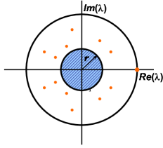
Figure 1: Schematic representation of the spectrum of ${\cal P\/}$. The dots represent the point spectrum ($\sigma_{\rm ps}$) while the circle of radius $r$ represents the essential spectrum.

Now assuming that the eigenvalues are nondegenerate (and that $r\ll 1$) then we can make an approximate spectral decomposition of ${\cal P}$ as

$${\cal P}\approx\sum_{i}\lambda_{i}{\cal R}_{i}({\cal L}_{i},\ .\ )$$ (44)

where ${\cal R}_{i}$, (${\cal L}_{i}$) are the right (left) eigenfunctions. Using this spectral decomposition explicitly in Eq. (42) we get an expansion of $C_{fg}$ like

$$C_{fg}(t)=\sum_{i}\lambda_{i}^{t}(f,{\cal R}_{i})({\cal L}_{i},g)$$ (45)

clearly dominated by the point spectrum $\sigma_{\rm ps}$. From Eq. (45) it is clear that in the limit $t\to\infty$ we have $C_{fg}(t)\sim\lambda_{1}^{t}(f,{\cal R}_{1})({\cal L}_{1},g)$, and the importance of the largest (in modulus) RP resonance becomes evident. The preceding analysis allows us to identify the complex eigenvalues $\lambda_{i}$ in the point spectrum of $\sigma_{\rm sp}$ of ${\cal P}$ with the RP resonances.

There are many methods (in use lately) to compute the classical PF spectrum. We briefly describe two of the most popular. The first one is a truncation method used for example by Manderfeldet al. manderfeld , Khodas et al. khodas , Hasegawa and Saphirhase and was nicely summerized by Fishmanfishman in the following way:

1. Introduce a basis ordered by increased resolution. Typically Fourier modes, Legendre polynomialshase or spherical harmonicsmanderfeld .

2. Truncate to a desired dimension $N$ leaving the rapidly oscillating components out. This acts as coarse graining of ${\cal P}$.

3. Compute the eigenvalues of the truncated operator and as $N$ is increased observe that there is a part that freezes and is independent of $N$.

4. Compare the frozen eigenvalues with the resonances obtained by analytic continuation of the resolvent.

It should be duly noted that this method was successfully implemented also for systems with a mixed phase spaceweber .

The second method consists of implementing a coarse grainingnonn ; agam of ${\cal P\/}$ by convoluting it with a Gaussian kernel of width $\epsilon$

$${\cal P}_{\epsilon}\stackrel{{\scriptstyle{\rm def}}}{{=}}{\cal D}_{\epsilon}\circ{\cal P\/}.$$ (46)

Essentially this is achieved by just replacing the delta functions in Eq. (41) by normalized (and periodized in the case of the torus) Gaussians of width $\epsilon$. This kind of coarse graining is equivalent to adding diffusive noise in the equations of motion.gaspard2 In order to perform the calculations a discretization of phase space is needed. The RP resonances are the eigenvalues of the coarse grained PF, ${\cal P}_{\epsilon}$, after doing an extrapolation of $N\to\infty$ and $\epsilon\to 0$.

VII.2 Spectrum of the Noisy Quantum Propagator

In a recent work Nonnenmachernonn proved the following theorem (which we state in a simplified form):

Theorem (Nonnenmachernonn ). For any smooth map on the torus and any fixed coarse graining parameter $\epsilon>0$, the spectrum of the coarse grained propagator $\text{{{S}}}_{\epsilon}=\text{{{D}}}_{\epsilon}\circ\text{{{U}}}$, converges in the classical limit $N\to\infty$ to the point spectrum of the classical coarse-grained propagator ${\cal P}_{\epsilon}={\cal D}_{\epsilon}\circ{\cal P}$.

Where both coarse grained propagators are like the ones described in the previos section and the noise is assumed to be Gaussian with characteristic width $\epsilon$.

Thus the introduction of noise in the quantum propagator makes the classical decay rates (RP resonances) emerge naturally. The problem which persists is the need to explore the large $N$ region because then the propagator of density matrices is a, much larger, $N^{2}\times N^{2}$ matrix. However the decays will be ruled by the largest eigenvalues (in modulus) so in fact only a small group of the leading of the eigenvalues is really relevant. In what follows we describe some methods used recently to compute the relevant part of the spectrum.

VIII Numerics

The goal is to explore regions of $N$ “large”. Thus the matrix to diagonalize, in principle, is $N^{2}\times N^{2}$. In the large $N$ limit this may represent a problem in terms of time and memory requirements. However, as was previously pointed out, only the largest eigenvalues (in modulus) play a significant role in the long time bahavior of observables. Therefore approximation methods can be used to significantly reduce the eigenvalue problem.

In what follows we describe three different methods to compute the leading spectrum. The first two are described briefly. They have the advantage that the only limitation on the number of eigenvalues to compute is the size of the matrices to digonalize. The third method, described in more detail, has the advantage that the first few (typically 10) eigenvalues can be computed with very small matrices (typically $10\times 10$).

VIII.1 Truncation Method:

Again, the truncation method described in Sec. VII.1 was succesfully used by Manderfeld et al. to obtain a nonunitary, coarse grained quantum propagator and to show that classical and quantum evolutions look alike (in the $N\to\infty$ limit) and that decay rates can be computed from the truncated propagator. However, this approach can have problems of interpretation if not of physical realizability. Spina and Saracenospina recently showed that when the quantum propagator is truncated in the way described, which is essentially a sharp truncation, the whole operation, unitary evolution followed by noise is not completely posititve and cannont be obtained as a quantum operation.

VIII.2 Chord Function Method:

On the other hand using the diffusive noise of Sec. VI and the chord representation a “smooth” truncation can be implemented (see Spina and Saracenospina and Aolita, et al. aolita ). Indeed the complete positivity is directly related to the positivity of the coeficients ${\cal C}_{\epsilon}(\alpha)$. Now since ${\cal C}_{\epsilon}(\alpha)$ is a (periodic) Gaussian then the spectrum $\widetilde{\cal C}_{\epsilon}(\beta)$ is also a Gaussian of complementary width (proportional to $1/\epsilon$). Therefore a large part of the elements of $\text{{{S}}}_{\epsilon}$ in the chord representation will be very small. If one sets for example the elements such that $\beta$ is larger than $1/(2\pi N)$ by some factor (bigger than one), exactly equal to zero, then, even though there will be oscillations in ${\cal C}_{\epsilon}(\alpha)$ (because it is the inverse DFT) they can be made negligibly small just by moving the truncation parameter. Using this method the matrices to diagonalize can be reduced to a dimension of order $N\times N$ and the precision obtained for the resonances is very good. The compromise lies in that using very small matrices to get the RP resonances means using very strong noise. So $N\times N$ is kind of a lower bound in the size of the eigenvalue problem to solve using the chord function method.

VIII.3 Iteration Method

The iteration method is a kind of variation of some known iteration methodsagam ; florido (e. g. Lanczos iteration methodgolub ). The main requirement is that the spectrum is of the form $1>|\lambda_{1}|\geq|\lambda_{2}|\geq\ldots\geq|\lambda_{k}|\geq\ldots$. The convergence depends strongly on the size of the gap $(1-|\lambda_{1}|)$. Consider the two sets of iterated states

$${\cal B}_{f}=\{\hat{\rho}_{0},\hat{\rho}_{1},\ldots,\hat{\rho}_{k},\ldots\};\ \ {\cal B}_{b}=\{\hat{\rho}_{0},\hat{\rho}_{-1},\ldots,\hat{\rho}_{-k},\ldots\}$$ (47)

where $\hat{\rho}_{0}$ is an arbitrary initial state and

$$\hat{\rho}_{k}=\text{{{S}}}_{\epsilon}^{k}\hat{\rho}_{0};\ \ \hat{\rho}_{-k}=\text{{{S}}}_{\epsilon}^{{\dagger}\,k}\hat{\rho}_{0}$$ (48)

Then we write a kind of projection of $\text{{{S}}}_{\epsilon}$ onto the subspace spanned by this (non-orthogonal) sets

$$\big{[}\text{{{S}}}_{\epsilon}\big{]}_{ij}=\mbox{Tr}(\hat{\rho}_{-i}^{\dagger}\text{{{S}}}_{\epsilon}\hat{\rho}_{j})$$ (49)

and solve the generalized eigenvalue equation

$$\text{Det}\left[\big{[}\text{{{S}}}_{\epsilon}\big{]}_{ij}-\lambda\big{[}\text{{{O}}}\big{]}_{ij}\right]=0$$ (50)

where $[\text{{{O}}}]_{ij}=\mbox{Tr}[\hat{\rho}_{-i}^{\dagger}\hat{\rho}_{j}]$ is the matrix of overlaps. Now if the spectrum has the required form, then both $[\text{{{S}}}_{\epsilon}]_{ij}$ and $[\text{{{O}}}]_{ij}$ decay very rapidly with $i,j$ so depending on the precision required a truncation size $k$ can be chosen. Typicaly in all the computations madegarma ; garma2 , for $N$ between 50 and 450, the matrices diagonalized where of sizes from $10\times 10$ to $15\times 15$. In Fig. 2 some results obtainedgarma ; garma2 with this method are displayed. The shaded region indicates the region in the prameters $N$ and $\epsilon$ inside which the spectrum stabilizes and can be considered classical. Care should be taken when approaching the limits $N\to\infty$ and $\epsilon\to 0$ because this limits do not commute. If $\epsilon$ goes to zero faster than $N$ to infinity then unitarity is recovered. There seems to be a kind of optimal function $\epsilon(N)$ to approach the classical limit. The fit is not easy to compute because it is very much system dependent.

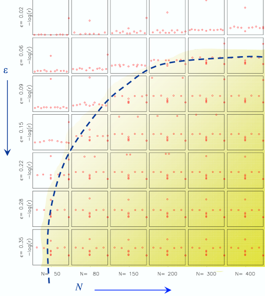
Figure 2: Spectrum of the propagator for the perturbed cat map ($k=0.01$) for different values of $\epsilon$ and $N$. The dashed line shows approximately the division in the space of the parameters between quantum (almost unitary) and noisy (almost classical) behavior.

In order to show that the values computed are the desired first $k$ largest eigenvalues we assume, for simplicity, that the spectrum is non-degenerate. The propagator can be written in its spectral decomposition form as

$$\text{{{S}}}_{\epsilon}\hat{\rho}=\sum_{i}\lambda_{i}\hat{R}_{i}\mbox{Tr}[\hat{L}_{i}^{\dagger}\hat{\rho}]$$ (51)

where $\hat{R}_{i}$ ( $\hat{L}_{i}$) is the right (left) eigenfunction. We can assume also that the overlap between the initial state $\rho_{0}$ and the right and left eigenfunctions is non-zero. Then Eq. (50) can be re-written as

$$\text{Det}[\mbox{\boldmath$\cal K$}^{T}(\text{{{S}}}_{\epsilon},\hat{\rho}_{0},k)\text{{{S}}}_{\epsilon}\mbox{\boldmath$\cal K$}(\text{{{S}}}_{\epsilon},\hat{\rho}_{0},k)-\lambda\mbox{\boldmath$\cal K$}^{T}(\text{{{S}}}_{\epsilon},\hat{\rho}_{0},k)\mbox{\boldmath$\cal K$}(\text{{{S}}}_{\epsilon},\hat{\rho}_{0},k)]=0$$ (52)

where $\mbox{\boldmath$\cal K$}(\text{{{S}}}_{\epsilon},\hat{\rho}_{0},k)$ is the Krylov matrix whose columns are the succesive iterates of the initial state $\hat{\rho}_{0}$ up to order $k$ (which is the truncation size we choose)

$$\mbox{\boldmath$\cal K$}(\text{{{S}}}_{\epsilon},\hat{\rho}_{0},k)=[\hat{\rho}_{0},\text{{{S}}}_{\epsilon},\hat{\rho}_{0},\ldots,\text{{{S}}}_{\epsilon}^{k-1}\hat{\rho}_{0}]$$ (53)

and $T$ denotes matrix transposition. Then using the expansion of $\hat{\rho}_{0}$ both in terms of $\hat{R}_{i}$ and $\hat{L}_{i}$ it can be showngarma2 that the determinant can be written as

$$\text{Det}[\mbox{\boldmath$\Lambda$}^{\dagger}\mbox{\boldmath$\Xi$}\mbox{\boldmath$\Lambda$}]=0$$ (54)

with

$$\mbox{\boldmath$\Lambda$}=\left(\begin{array}[]{ccccc}1&\lambda_{0}&\lambda_{0}^{2}&\cdots&\lambda_{0}^{k-1}\\ 1&\lambda_{1}&\lambda_{1}^{2}&\cdots&\lambda_{1}^{k-1}\\ \vdots&\vdots&\vdots&\ddots&\vdots\\ 1&\lambda_{k-1}&\lambda_{k-1}^{2}&\cdots&\lambda_{k-1}^{k-1}\end{array}\right)$$ (55)

and

$$\mbox{\boldmath$\Xi$}=\left(\begin{array}[]{cccc}\alpha_{0}\beta_{0}(\lambda_{0}-z)&0&\cdots&0\\ 0&\alpha_{1}\beta_{1}(\lambda_{1}-z)&\cdots&0\\ \vdots&\vdots&\ddots&\vdots\\ 0&\cdots&0&\alpha_{k-1}\beta_{k-1}(\lambda_{k-1}-z)\end{array}\right).$$ (56)

Now $\Lambda$ is a Vandermonde matrix and from m the asumption of non-degeneracy, the determinant is non-zero. Thus the solution of Eq. (54) is just given by the zeros of the determinant of $\Xi$ which are exactly the desired first $k$ eigenvalues. Even though we do not discuss precision we can say that the efficiency of the method depends mainly on two things. First, there has to be a finite gap between 1 and $\lambda_{1}$. The second, and very important also, is that the map should be easy to implement without constructing the whole $N^{2}\times N^{2}$ superoperator.

VIII.4 Long time behavior

Exponential stretching (with the rate given by the Lyapunov exponent) is the cause that correspondence is lost much faster than for regular systems. This discrepancy is observed in phase space quasi-probability distributions such as the Wigner functiondittrich ; kolovsky in the form of sub-Planck structure.zurekRMP For isolated systems, the characteristic time for the loss of correspondence in the Wigner function is usually called Eherenfestberman time. It is generally a very short time and can be expressed as $\tau_{E}=\lambda^{-1}\ln(S/\hbar)$, where $\lambda$ is the largest Lyapunov exponent and $S$ is some characteristic action.

Zurek and Paz conjecturedzurek that loss of correspondence in chaotic systems would be recovered by introducing decoherence. Moreover they stated that initially the linear entropy

$$S_{n}=-\ln\left[\mbox{Tr}[\hat{\rho}_{n}^{2}]\right],$$ (57)

(which is the natural logarithm of the purity) should grow linearly with $n$ (i.e. time), with a slope given by the largest lyapunov exponent of the corresponding classical system. This lyapunov behavior would have to be independent of the coupling strengh, that is the strengh of the noise, for a large range of values of the coupling. This statement was verified numericallybianucci ; garma . The lyapunov growth takes place until the Eherenfest time. Then the linear entropy saturates asymptotically to the value $\ln(N)$ that corresponds to the maximally mixed state $\hat{\rho}_{\infty}=\hat{I}/N$.

Another quantity of interest with similar short time behavior is the Loschmidt echo. It was proposedperes as a measure of irreversibility and could be used to characterize quantum chaos. Many recent worksjalabert ; losch show that the lyapunov regime indeed exists for classically chaotic systems. This quantity gained interes recently in the context of quantum information because of its close relation to fidelity.

There is yet another classical regime that can be identified. If we assume that there are nondegeneracies then in analogy Eq. (44) a spectral decomposition can be made but for the quantum noisy propagator

$$\text{{{S}}}_{\epsilon}\hat{\rho}=\sum_{i=0}^{N^{2}}\lambda_{i}\mbox{Tr}\left[\hat{L}_{i}^{\dagger}\,\hat{\rho}\right]\,\hat{R}_{i}$$ (58)

where $\hat{R}_{i}$ and $\hat{L}_{i}$ are the right and left eigenoperators of $\text{{{S}}}_{\epsilon}$, and the eigenvalues are ordered by decreasing modulus (starting with $\lambda_{0}=1$). Then, for example, the autocorrelation function behaves asymptotically as

$$C_{n} = \mbox{Tr}\left[\hat{\rho}_{0}\hat{\rho}_{n}\right]-\mbox{Tr}\left[{\hat{I}\over N}\hat{\rho}_{0}\right]^{2}$$ (59)

$$= \lambda_{0}\,\mbox{Tr}\left[\hat{\rho}_{0}\hat{\rho}_{\infty}\right]\mbox{Tr}\left[\hat{\rho}_{\infty}\hat{\rho}_{0}\right]+\sum_{i=1}^{N^{2}}\lambda_{i}^{n}\mbox{Tr}\left[\hat{\rho}_{0}\hat{R}_{i}\right]\mbox{Tr}\left[\hat{L}_{i}^{\dagger}\hat{\rho}_{0}\right]-{1\over N^{2}}$$

$$\sim \lambda_{1}^{n}\,\mbox{Tr}\left[\hat{\rho}_{0}\hat{R}_{1}\right]\mbox{Tr}\left[\hat{L}_{1}^{\dagger}\hat{\rho}\right].$$

where $\lambda_{0}=1$ and $\hat{\rho}_{\infty}$ as defined in Eq. (34). In Table 1 the long time behavior of the autocorrelation function, the linear entropy (logarithm of the purity) and the Loschmidt echo is summerized. In all cases the logarithm grows linearly with time ($n$) and the slope is determined by $\lambda_{1}$. Now taking $N$ and $\epsilon$ in the correct region of Fig. 2, $\lambda_{1}$ is identified with the largest RP resonance of the classical system. Thus another classical property has emerged from the quantum system by the addition of noise.

Quantity	Definition	Aymptotic behavior	Ln
Autocorrelation	$\mbox{Tr}[\hat{\rho}_{0}\hat{\rho}_{n}]-1/N$	$\sim\ \lambda_{1}^{n}$	$\sim\ n\lambda_{1}$
Linear Entropy	$-\ln[\mbox{Tr}[\hat{\rho}_{n}^{2}]]$	$\sim\ -2n\ln[\lambda_{1}]$	$\sim\ -2n\ln[\lambda_{1}]$
Loschmidt echo	$\mbox{Tr}[\hat{\rho}_{n}\hat{\rho}^{\prime}_{n}]$	$\sim\ \lambda_{1}^{n}(\lambda^{\prime}_{1})^{n}$	$\sim\ n(\lambda_{1}+\lambda_{1}^{\prime})$

Table 1: Long time ehavior of the aurotcorrelation function$C_{n}$, the linear entropy $S_{n}$ and the Loschmidt echo $M_{n}$. In the case of $S_{n}$ and $M_{n}$ we measure the approach to equilibrium and for tah purpose we explicitly subtracted the invariant state $\rho_{\infty}$ in order to avoid saturation.

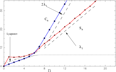
Figure 3: Time evolution of the linear entropy $S_{n}$ (diamonds) and the autocorrelation function (triangles). The points result from the average of ten initial conditions corresponding to coherent states centered at ten different points. The Dot-Dash-Dot line indicates the initial Lyapunov behavior and the Dashed lines indicate the RP behavior. The slopes of the RP lines were obtained from the leading eignvalue computed using the iteration method. As it was expected, the slope for $S_{N}$ is exactly two times the slope of $C_{n}$. The dotted line shows the behavior if the uniform density is not subtracted.

The long time linear regime can be best observed in Fig. 3 where $C_{n}$ and $S_{n}$ are plotted. In order to uncover the long time regime for $S_{n}$ we subtracted $\rho_{\infty}$ from the initial states. The initial Lyapunov regime is very well observed for $S_{n}$ and for longer times the RP regime is also well defined. The fact that $C_{n}$ has no Lyapunov regime is well understood. For a chaotic system the overlap between the initial state and the succesive iterates is a highly fluctuating function until after the Eherenfest time (in which the phase space distribution has reached the edges of phase space). This is the reason why we averaged over a number of initial states in order to get a smoother function. The time graphs for the Loschmidt echo are very similar

IX Concluding remarks

Using some new numerical methods we established quantum classical correspondence for chaotic quantum maps throught the spectrum of the coarse-grained propagator. For a wide range of parameters, the spectrum could be related to the classical Ruelle Pollicott resonances. Many techniques to compute the spectrum where presented and some of the advantages of the iteration method (mainly for chaotic systems) could be appreaciated. As an open question there remains the issue of establishing an optimal relation betwwen the noise strength $\epsilon$ and $\hbar$ ($N$) so that the classical limit can be attainedcorrectly. Recent worktoscano provides an expression such relation in the context of correspondence-breaking time. Although it looks promising we have no conclusive proof of its relation to the spectrum.

References

- (1) W. H. Zurek, Rev. Mod. Phys. 75, 715 (2003), and references therein.
- (2) M. C. Gutzwiller, Chaos in Classical and Quantum Mechanics (Springer, New York, 1990).
- (3) Cvitanović et al. Classcal and Quantum Chaos: a Cyclist Treatise (Copenhagen, www.nbi.dk/ChaosBook/).
- (4) E. G. Vergini (1999), J. Phys. A33, 4709 (2000); E. G. Vergini and G. Carlo, J. Phys. A33, 4717 (2000).
- (5) E. J. Heller, Phys. Rev. Lett. 53, 1515 (1984).
- (6) O. Bohigas, in Chaos and Quantum Physics, edited by M.-J. Giannoni, A. Voros, and J. Zinn-Justin (elsevier Science, New York, 1990).
- (7) G. P. Berman and G. M. Zaslavsky, Physica A91, 450 (1978).
- (8) P. Bianucci, J. P. Paz and M. Saraceno Phys. Rev. E 65, 046226 (2002).
- (9) I. García-Mata, M. Saraceno, and M. E. Spina, Phys. Rev. Lett. 91, 064101 (2003).
- (10) R. A. Jalabert and H. M. Pastawski, Phys. Re. Lett. 86, 2490 (2001).
- (11) To cite only a few see: Silverstrov and C. W. J. Beenakker. Phys. Rev. E 64 055203(R) (2001); F. M. Cucchietti, H. M. Pastawski and D. A. Wisniacki. Phys. Rev. E 65,045206 (2002); G. Benenti and G. Casati. Phys. Rev. E 65, 066205 (2002); F.M. Cucchietti, D.A.R. Dalvit, J. P. Paz and W.H. Zurek, Phys. Rev. Lett. 91, 210403 (2003).
- (12) I. García-Mata and M. Saraceno, Phys. Rev. E69, 056211 (2004)
- (13) M. L. Aolita, I. García-Mata, and M. Saraceno, Phys. Rev. A70, 062301 (2004).
- (14) J. Schwinger, Proc. Natl. Acad. Sci. U.S.A. 46, 570 (1960); 46, 893 (1960).
- (15) J. Bertrand and P. Bertrand, Found. Phys. 17 397 (1987)
- (16) J. H. Hannay and M. V. Berry, Physica 1D,267-290 (1980).
- (17) A.M. Ozorio de Almeida Phys. Rep. 295 266 (1998); A. Rivas and A. M. Ozorio de Almeida, Ann. Phys. (N.Y.)276, 223 (1999).
- (18) W. K. Wooters, Ann. Phys. (NY) 176,1 (1987).
- (19) C. Miquel, J. P. Paz and M. Saraceno, Phys. Rev. A65, 2309 (2002).
- (20) C. Miquel, J. P. Paz, M. Saraceno, E. Knill, R. Laflamme, and C. Negrevergne, Nature (London) 418, 59 (2002).
- (21) V. Gorini, A. Kossakowski and E.C.G Sudarshan, J. Math. Phys. 17, 821 (1972).
- (22) G. Lindblad, Commun. Math Phys 48, 119 (1976).
- (23) J. Preskill. “1998 Lecture Notes for Physics 229: Quantum Information and Computation” available at http://www.theory.caltech.edu/people/preskill
- (24) I. Chuang and M. Nielsen. Quantum Information and Computation (Cambridge University Press, Cambridge, UK, 2001).
- (25) K. Kraus, States, Effects and Operations (Springer-Verlag, Berlin, 1983).
- (26) M. Moshinsky and C. Quesne J. Math. Phys 12, 1772 (1971).
- (27) See, for example, A. M. Ozorio de Almeida, Hamiltonian Systems: Chaos and Quantization (Cambridge University Press, Cambridge, 1988).
- (28) M. Basilio de Matos and A. M. Ozorio de Almeida, Ann. Phys. 237, 46-65 (1995)
- (29) M. L. Balazs and A. Voros, Ann. Phys. 190,1 (1989).
- (30) M. Saraceno,Ann. Phys. 99, 37 (1990).
- (31) F. M. Izrailev, Phys. Rev. Lett. 56, 541 (1986).
- (32) M. V. Berry, N. L. Balazs, M. Tabor and A. Voros, Ann. Phys. (NY) 122, 26 (1979).
- (33) G. Palla, G. Vattay, and A. Voros, Phys. Rev. E64, 012104 (2001).
- (34) D. Braun, CHAOS 9,730 (1999) and D. Braun, Physica D, 131, 265 (1999); D. Braun, Dissipative Quantum Chaos and Decoherence (Springer-Verlag, Berlin, 2001).
- (35) S. Nonnenmacher, Nonlinearity 16, pp.1685-1713 (2003).
- (36) See T. Wellens and A. Buchleitner in Lecture Notes in Physics: Dynamics of Disipation, edited by P. Garbaczewski and R. Olkiewicz, (Springer-Verlag, Berlin, 2002), and references therein.
- (37) C. Manderfeld, J. Weber and F. Haake, J. Phys. A34, 9893 (2001).
- (38) K. Pance, W. Lu and S. Sridhar, Phys rev. Lett 85, 2737 (2000).
- (39) D. Ruelle, Phys. Rev. Lett. 56, 405 (1986); D. Ruelle, J. Stat. Phys 44, 281 (1986).
- (40) V. Baladi, J. P. Eckmann and D. Ruelle, Nonlinearity 2, 119 (1989)
- (41) F. Christiansen, G. Paladin and H. H. Rugh, Phys. Rev. Lett. 65, 2087 (1990).
- (42) P. Gaspard and D. Alonso Ramirez, Phys. Rev. A45, 8383 (1992).
- (43) F. Brini, S. Siboni, G. Turchetti and S. Valenti, Nonlinearity 10, 1257 (1997).
- (44) M. Blank, G. Keller and C. Liverani, Nonlinearity 15, 1905 (2002).
- (45) H. H. Rugh, Nonlinearity 5, 1237-1263 (1992).
- (46) M. Khodas, S. Fishman, and O. Agam, Phys. Rev. E62, 4769 (2000).
- (47) H. H. Hasegawa and W. C. Saphir, Phys. Rev. A46, 7401 (1992).
- (48) S. Fishman and S. Rahav, in Lecture Notes in Physics: Dynamics of Disipation, edited by P. Garbaczewski and R. Olkiewicz, (Springer-Verlag, Berlin, 2002).
- (49) J. Weber, F. Haake, P.A. Braun, C. Manderfeld and P. Šeba, J. Phys. A34, 7195 (2001).
- (50) G. Blum and O. Agam, Phys. Rev. E62, 1977 (2000).
- (51) P. Gaspard, G. Nicolis and A. Provata, Phys. Rev. E51, 74 (1995).
- (52) M. E. Spina and M. Saraceno, J. Phys. A: Math. Gen. 37, L415 (2004).
- (53) See for example: P. Pechukas, Phys. Rev. Lett 73, 1060 (1994); R. Alicki, (Comment) Phys. Rev. Lett 75, 3020 (1995); P. Pechukas (Reply) Phys. Rev. Lett 75, 3021 (1995).
- (54) G. H. Goloub and C. F. Van Loan, Matrix Computations (The Johns Hopkins University Press, Baltimore, 1996).
- (55) R. Florido, J. M. Martín-González and J. M. Gómez Llorente, Phys. Rev. E66, 046208 (2002).
- (56) T. Dittrich and R. Graham, Europhys. Lett. 7, 287 (1988)
- (57) A. R. Kolovsky, CHAOS 6, 534 (1996).
- (58) W. H. Zurek and J. P. Paz, Phys. Rev. Lett. 72, 2508 (1994).
- (59) A. Peres, Phys. Rev. A 30, 1610 (1984).
- (60) F. Toscano, R. L. de Matos Filho and L. Davidovich, Phys. Rev. A 71, 010101 (2005).