Effective potential analytic continuation approach
for real time quantum correlation functions involving nonlinear operators

Abstract

We apply the effective potential analytic continuation (EPAC) method to the calculation of real time quantum correlation functions involving operators nonlinear in the position operator $\hat{q}$. For a harmonic system the EPAC method provides the exact correlation function at all temperature ranges, while the other quantum dynamics methods, the centroid molecular dynamics and the ring polymer molecular dynamics, become worse at lower temperature. For an asymmetric anharmonic system, the EPAC correlation function is in very good agreement with the exact one at $t=0$. When the time increases from zero, the EPAC method gives good coincidence with the exact result at lower temperature. Finally, we propose a simplified version of the EPAC method to reduce the computational cost required for the calculation of the standard effective potential.

I INTRODUCTION

The imaginary time path integral fh has provided a useful framework suitable for numerical analyses of quantum statistical-mechanical systems. Most of the static properties of quantum systems can be calculated by means of the path integral Monte Carlo (PIMC) or path integral molecular dynamics (PIMD) technique bt ; ce . However, it is not straightforward to apply the PIMC/PIMD methods to computing dynamical properties such as the real time quantum correlation function $\langle\hat{A}(t)\hat{B}(0)\rangle_{\beta}$. This is because it is nontrivial to construct real time quantities from a finite number of imaginary time data obtained numerically tb . To overcome such difficulty, a number of promising methods of numerical analytic continuation based on the maximum entropy method have been proposed and applied to various many-body systems si ; gb ; rr ; rr1 .

Recently, the centroid molecular dynamics (CMD) method cv , the ring polymer molecular dynamics (RPMD) method cm , and the effective potential analytic continuation (EPAC) method hk1 have been proposed as new quantum dynamics methods to calculate real time quantum correlation functions at finite temperature. Both the CMD and the RPMD are the methods to calculate the canonical (Kubo-transformed) correlation function kubo $\langle\hat{A}(t)\hat{B}(0)\rangle_{\beta}^{\rm can}$ by means of molecular dynamics techniques. On the other hand, the EPAC is a method to obtain the real time quantum correlation function $\langle\hat{A}(t)\hat{B}(0)\rangle_{\beta}$ by means of the effective action formalism ep ; riv ; ps and an analytic continuation procedure bell . It has been shown analytically that all these methods are exact in harmonic systems for the real time quantum correlation functions of a linear function of the position operator, $\hat{A}=\hat{B}=\hat{q}$ jv ; cm ; hk2 . However, for nonlinear operators such as $\hat{A}=\hat{B}=\hat{q}^{n}$, it is nontrivial whether these quantum dynamics methods yield the exact result even in harmonic systems jv ; cm . This is the nonlinear operator problem in quantum dynamics methods.

From a practical point of view, the nonlinear operator problem is a quite important subject to be tackled. In many problems of chemical interest, the real time correlation functions of nonlinear operators are often needed for the calculation of various dynamical properties McQ . For example, the CMD has been applied to the calculation of the transport coefficients such as thermal conductivity, shear viscosity, and bulk viscosity of quantum liquid parahydrogen appli . Here it is found that the calculated transport properties are in good agreement with the experimental data. However, there is no rigorous theoretical basis for applying the CMD method to such properties represented by means of the correlation functions involving operators nonlinear in $\hat{q}$ (or momentum operator $\hat{p}$). Therefore we need, in general, a quantum dynamics method which is theoretically valid even for the time correlation functions of nonlinear operators.

The present status of the nonlinear operator problem in the three quantum dynamics methods, CMD, RPMD, and EPAC, is summarized as follows. For the CMD method, Reichman et al. have argued this problem in their pioneering paper to conclude that a CMD correlation function involving nonlinear operators corresponds to a higher-order Kubo-transformed correlation function reich . On the other hand, Craig and Manolopoulos have shown that the RPMD is exact for all the operators involving $\hat{q}$ in the limit $t\to 0$ cm . As for our EPAC method, the nonlinear operator problem has not been examined yet. In addition to these three methods, a theoretical approach based on the quantum mode-coupling theory has been applied to study the dynamical properties involving nonlinear operators in quantum liquids rr1 ; rr2 .

In the present paper, we develop the method of the EPAC for the calculation of the real time quantum correlation function involving the nonlinear operator $\hat{A}=\hat{B}=\hat{q}^{n}$. As a simple example, at first we show the EPAC correlation function $\langle\hat{q}^{2}(t)\hat{q}^{2}(0)\rangle_{\beta}^{EPAC}$ for a harmonic oscillator comparing with the results of the CMD and the RPMD. Next we calculate $\langle\hat{q}^{2}(t)\hat{q}^{2}(0)\rangle_{\beta}^{EPAC}$ numerically in an asymmetric anharmonic system. We also propose a simplified EPAC method to reduce the computational cost required in the EPAC calculation.

In Sec. II, we summarize the effective action formalism and present how to calculate the EPAC correlation function involving nonlinear operators. The results for a harmonic oscillator are given in Sec. III. Numerical results for an anharmonic oscillator are shown in Sec. IV. In this section we also present the simplified EPAC method. The conclusions are given in Sec. V.

II EFFECTIVE POTENTIAL ANALYTIC CONTINUATION METHOD FOR NONLINEAR OPERATORS

Hereafter we treat the real time quantum autocorrelation function of the nonlinear operator $\hat{q}^{n}$, $~{}\langle\hat{q}^{n}(t)\hat{q}^{n}(0)\rangle_{\beta}$. In principle, this can be obtained from the imaginary time Green function $\langle T\hat{q}^{n}(\tau)\hat{q}^{n}(0)\rangle_{\beta}$ via an analytic continuation procedure bell . Here $T$ represents a time-ordered product. On the other hand, it is known that the Green function $\langle T\hat{q}^{n}(\tau)\hat{q}^{n}(0)\rangle_{\beta}$ is given as a special case of $2n$-point imaginary time Green function $\langle T\hat{q}(\tau_{1})\cdot\cdot\cdot\hat{q}(\tau_{2n})\rangle_{\beta}$, which can be constructed from the standard effective potential $V_{\beta}(Q)$ appearing in the effective action formalism ep ; riv ; ps . Consequently, the real time quantum correlation function $\langle\hat{q}^{n}(t)\hat{q}^{n}(0)\rangle_{\beta}$ should be obtained by means of the effective action formalism and the analytic continuation. A series of these procedures is the EPAC method for the nonlinear operator $\hat{q}^{n}$, which we newly show in this section. As the simplest example, we present the EPAC calculation of the autocorrelation function of the quadratic operator $\hat{q}^{2}$, $\langle\hat{q}^{2}(t)\hat{q}^{2}(0)\rangle_{\beta}$, in Secs. IIA and IIB.

II.1 Effective action formalism for multipoint Green functions

We begin with the effective action formalism ep ; riv ; ps . Consider a quantum system where a quantum particle of mass $m$ moves in a one-dimensional potential $V(q)$ at inverse temperature $\beta$. The quantum canonical partition function of this system is expressed in terms of the imaginary time path integral

$${\cal Z}_{\beta}[J] = \int^{\infty}_{-\infty}dq\int^{q(\beta\hbar)=q}_{q(0)=q}{\cal D}q~{}\!\exp\left[-S_{E}/\hbar+\int^{\beta\hbar}_{0}d\tau J(\tau)q(\tau)/\hbar\right],$$ (1)

where $S_{E}$ is the Euclidean action functional

$$S_{E}[q]=\int^{\beta\hbar}_{0}d\tau\left[~{}\!\frac{1}{2}~{}\!m~{}\!\dot{q}^{2}+V(q)~{}\!\right],$$ (2)

and $J(\tau)$ is an external source. The generating functional $W_{\beta}[J]$ is defined as

$$W_{\beta}[J] = \hbar\log{\cal Z}_{\beta}[J].$$ (3)

The functional derivative of $W_{\beta}[J]$ with respect to $J(\tau)$ produces the quantum statistical-mechanical expectation value of the operator $\hat{q}$ in the presence of $J$,

$$\frac{\delta W_{\beta}[J]}{\delta J(\tau)} = \langle\hat{q}(\tau)\rangle_{\beta}^{J}\equiv Q(\tau).$$ (4)

The effective action $\Gamma_{\beta}[Q]$ is defined by the Legendre transform of $W_{\beta}[J]$,

$$\Gamma_{\beta}[Q] = -W_{\beta}[J]+\int^{\beta\hbar}_{0}d\tau J(\tau)Q(\tau),$$ (5)

which satisfies the quantum-mechanical Euler-Lagrange equation $\delta\Gamma_{\beta}[Q]/\delta Q(\tau)=J(\tau)$. The exact quantum statistical-mechanical expectation value $Q_{S}(\tau)$($=\langle\hat{q}(\tau)\rangle_{\beta}$) is obtained as a solution of the equation

$$\frac{\delta\Gamma_{\beta}[Q]}{\delta Q(\tau)}=0.$$ (6)

Note that the expectation value $Q_{S}(\tau)$ is independent of imaginary time $\tau$ in thermal equilibrium.

The $n$-point connected Green function $G_{\beta}^{C}(\tau_{1},...,\tau_{n})$ is generated by the $n$th-order functional derivative of $W_{\beta}[J]$ with respect to $J(\tau)$ riv ; ps . For example, the two-point connected Green function is given by

$$G_{\beta}^{C}(\tau_{1}-\tau_{2}) = \hbar\left.\frac{\delta^{2}W_{\beta}[J]}{\delta J(\tau_{1})\delta J(\tau_{2})}\right|_{J=0}$$ (7)

$$= \langle T\hat{q}(\tau_{1})\hat{q}(\tau_{2})\rangle_{\beta}-\langle\hat{q}(\tau_{1})\rangle_{\beta}~{}\!\langle\hat{q}(\tau_{2})\rangle_{\beta}.$$

Then we obtain the two-point Green function

$$\langle T\hat{q}(\tau_{1})\hat{q}(\tau_{2})\rangle_{\beta}=G_{\beta}^{C}(\tau_{1}-\tau_{2})+Q_{S}(\tau_{1})Q_{S}(\tau_{2}).$$ (8)

The procedure in Eqs. (1)-(8) has been described in Ref. hk1, . In a similar way, the three- and four-point Green functions can be explicitly expressed as

$$\langle T\hat{q}(\tau_{1})\hat{q}(\tau_{2})\hat{q}(\tau_{3})\rangle_{\beta} = \hbar^{2}\left.\frac{\delta^{3}W_{\beta}[J]}{\delta J(\tau_{1})\delta J(\tau_{2})\delta J(\tau_{3})}\right|_{J=0}$$ (9)

$$+Q_{S}(\tau_{1})\langle T\hat{q}(\tau_{2})\hat{q}(\tau_{3})\rangle_{\beta}+(1\leftrightarrow 2)+(1\leftrightarrow 3)$$

$$-~{}2~{}Q_{S}(\tau_{1})Q_{S}(\tau_{2})Q_{S}(\tau_{3}),$$

$$\langle T\hat{q}(\tau_{1})\hat{q}(\tau_{2})\hat{q}(\tau_{3})\hat{q}(\tau_{4})\rangle_{\beta} = \hbar^{3}\left.\frac{\delta^{4}W_{\beta}[J]}{\delta J(\tau_{1})\delta J(\tau_{2})\delta J(\tau_{3})\delta J(\tau_{4})}\right|_{J=0}$$ (10)

$$\!\!\!\!\!\!\!\!\!\!\!\!\!\!\!+\hbar^{2}Q_{S}(\tau_{1})\left.\frac{\delta^{3}W_{\beta}[J]}{\delta J(\tau_{2})\delta J(\tau_{3})\delta J(\tau_{4})}\right|_{J=0}+(1\leftrightarrow 2)+(1\leftrightarrow 3)+(1\leftrightarrow 4)$$

$$\!\!\!\!\!\!\!\!\!\!\!\!\!\!\!+\langle T\hat{q}(\tau_{1})\hat{q}(\tau_{2})\rangle_{\beta}\langle T\hat{q}(\tau_{3})\hat{q}(\tau_{4})\rangle_{\beta}+(2\leftrightarrow 3)+(2\leftrightarrow 4)$$

$$\!\!\!\!\!\!\!\!\!\!\!\!\!\!\!-~{}2~{}Q_{S}(\tau_{1})Q_{S}(\tau_{2})Q_{S}(\tau_{3})Q_{S}(\tau_{4}),$$

respectively. Here $(i\leftrightarrow j)$ denotes the interchange of $\tau_{i}$ with $\tau_{j}$.

On the other hand, the $n$th-order functional derivative $\delta^{n}W_{\beta}/\delta J^{n}$ is connected with the $n$th-order functional derivative of the effective action $\delta^{n}\Gamma_{\beta}/\delta Q^{n}$ ps ,

$$\left.\frac{\delta^{2}W_{\beta}[J]}{\delta J(\tau_{1})\delta J(\tau_{2})}\right|_{J=0} = \left(\left.\frac{\delta^{2}\Gamma_{\beta}[Q]}{\delta Q(\tau_{1})\delta Q(\tau_{2})}\right|_{Q=Q_{S}}\right)^{-1},$$ (11)

$$\left.\frac{\delta^{3}W_{\beta}[J]}{\delta J(\tau_{1})\delta J(\tau_{2})\delta J(\tau_{3})}\right|_{J=0} = -\frac{1}{\hbar^{3}}\int^{\beta\hbar}_{0}\!\!\!\!\!ds_{1}\int^{\beta\hbar}_{0}\!\!\!\!\!ds_{2}\int^{\beta\hbar}_{0}\!\!\!\!\!ds_{3}$$ (12)

$$\times G_{\beta}^{C}(s_{1}-\tau_{1})G_{\beta}^{C}(s_{2}-\tau_{2})G_{\beta}^{C}(s_{3}-\tau_{3})$$

$$\times\left.\frac{\delta^{3}\Gamma_{\beta}[Q]}{\delta Q(s_{1})\delta Q(s_{2})\delta Q(s_{3})}\right|_{Q=Q_{S}},$$

$$\left.\frac{\delta^{4}W_{\beta}[J]}{\delta J(\tau_{1})\delta J(\tau_{2})\delta J(\tau_{3})\delta J(\tau_{4})}\right|_{J=0} = -\frac{1}{\hbar^{4}}\int^{\beta\hbar}_{0}\!\!\!\!\!ds_{1}\int^{\beta\hbar}_{0}\!\!\!\!\!ds_{2}\int^{\beta\hbar}_{0}\!\!\!\!\!ds_{3}\int^{\beta\hbar}_{0}\!\!\!\!\!ds_{4}$$ (13)

$$\times G_{\beta}^{C}(s_{1}-\tau_{1})G_{\beta}^{C}(s_{2}-\tau_{2})G_{\beta}^{C}(s_{3}-\tau_{3})G_{\beta}^{C}(s_{4}-\tau_{4})$$

$$\times\left.\frac{\delta^{4}\Gamma_{\beta}[Q]}{\delta Q(s_{1})\delta Q(s_{2})\delta Q(s_{3})\delta Q(s_{4})}\right|_{Q=Q_{S}}$$

$$\!\!\!\!\!\!\!\!\!\!\!\!\!\!\!\!\!\!\!\!+\frac{1}{\hbar^{5}}\int^{\beta\hbar}_{0}\!\!\!\!\!ds_{1}\int^{\beta\hbar}_{0}\!\!\!\!\!ds_{2}\int^{\beta\hbar}_{0}\!\!\!\!\!ds_{3}\int^{\beta\hbar}_{0}\!\!\!\!\!ds_{4}\int^{\beta\hbar}_{0}\!\!\!\!\!du\int^{\beta\hbar}_{0}\!\!\!\!\!dv$$

$$\!\!\!\!\!\!\!\!\!\!\!\!\!\!\!\!\!\!\!\!\times G_{\beta}^{C}(s_{1}-\tau_{1})G_{\beta}^{C}(s_{2}-\tau_{2})G_{\beta}^{C}(u-v)G_{\beta}^{C}(s_{3}-\tau_{3})G_{\beta}^{C}(s_{4}-\tau_{4})$$

$$\!\!\!\!\!\!\!\!\!\!\!\!\!\!\!\!\!\!\!\!\times\left.\frac{\delta^{3}\Gamma_{\beta}[Q]}{\delta Q(s_{1})\delta Q(s_{2})\delta Q(u)}\right|_{Q=Q_{S}}\!\!\!\!\cdot~{}\left.\frac{\delta^{3}\Gamma_{\beta}[Q]}{\delta Q(v)\delta Q(s_{3})\delta Q(s_{4})}\right|_{Q=Q_{S}}$$

$$\!\!\!\!\!\!\!\!\!\!\!\!\!\!\!\!\!\!\!\!+(2\leftrightarrow 3)+(2\leftrightarrow 4).$$

Using Eqs. (7)-(13), we can construct the imaginary time Green functions in terms of the effective action $\Gamma_{\beta}[Q]$.

Now we employ the local potential approximation (LPA) to the effective action,

$$\Gamma_{\beta}[Q] = \int^{\beta\hbar}_{0}d\tau\left[V_{\beta}(Q)+\frac{1}{2}~{}\!m~{}\!\dot{Q}^{2}\right],$$ (14)

where $V_{\beta}(Q)$ is the standard effective potential, i.e., the leading order of the derivative expansion of $\Gamma_{\beta}[Q]$ ep ; riv ; ps . For the case $Q_{S}(\tau)$ is $\tau$ independent, Eq. (6) becomes the stationary condition $\left.{\partial V_{\beta}}/{\partial Q}\right|_{Q=Q_{\rm min}}=0$, which determines the expectation value $Q_{S}(\tau)$ as the standard effective potential minimum $Q_{\rm min}$. Then the functional derivatives of the effective action $\delta^{n}\Gamma_{\beta}/\delta Q^{n}$ become

$$\left.\frac{\delta^{2}\Gamma_{\beta}[Q]}{\delta Q(\tau_{1})\delta Q(\tau_{2})}\right|_{Q=Q_{S}} = \left(-m\frac{d^{2}}{d\tau^{2}}+\left.\frac{\partial^{2}V_{\beta}}{\partial Q^{2}}\right|_{Q=Q_{\rm min}}\right)\delta(\tau_{1}-\tau_{2}),$$ (15)

$$\left.\frac{\delta^{3}\Gamma_{\beta}[Q]}{\delta Q(\tau_{1})\delta Q(\tau_{2})\delta Q(\tau_{3})}\right|_{Q=Q_{S}} = \left.\frac{\partial^{3}V_{\beta}}{\partial Q^{3}}\right|_{Q=Q_{\rm min}}\delta(\tau_{1}-\tau_{2})\delta(\tau_{1}-\tau_{3}),$$ (16)

$$\left.\frac{\delta^{4}\Gamma_{\beta}[Q]}{\delta Q(\tau_{1})\delta Q(\tau_{2})\delta Q(\tau_{3})\delta Q(\tau_{4})}\right|_{Q=Q_{S}} = \left.\frac{\partial^{4}V_{\beta}}{\partial Q^{4}}\right|_{Q=Q_{\rm min}}\delta(\tau_{1}-\tau_{2})\delta(\tau_{1}-\tau_{3})\delta(\tau_{1}-\tau_{4}).$$ (17)

If we expand $V_{\beta}$ around the minimum $Q=Q_{\rm min}$,

$$V_{\beta}(Q)=\sum_{n=0}^{\infty}\frac{a_{n}}{n!}(Q-Q_{\rm min})^{n},$$ (18)

then the derivatives of $V_{\beta}$ appearing in Eqs. (15)-(17) are given as the coefficients in the series, $a_{n}=\partial^{n}V_{\beta}/\partial Q^{n}|_{Q=Q_{\rm min}}$.

II.2 EPAC method

Now we proceed to the calculations of the real time quantum correlation function $\langle\hat{q}^{2}(t)\hat{q}^{2}(0)\rangle_{\beta}$, i.e., the aim of the present paper. First, by setting $\tau_{1}=\tau_{2}=\tau~{}(0\leq\tau\leq\beta\hbar)$ and $\tau_{3}=\tau_{4}=0$ in Eq. (10), we obtain the imaginary time Green function

$$\langle T\hat{q}^{2}(\tau)\hat{q}^{2}(0)\rangle_{\beta} = \hbar^{3}\left.\frac{\delta^{4}W_{\beta}[J]}{\delta J(\tau)\delta J(\tau)\delta J(0)\delta J(0)}\right|_{J=0}$$ (19)

$$+ 2\hbar^{2}Q_{\rm min}\left[\left.\frac{\delta^{3}W_{\beta}[J]}{\delta J(\tau)\delta J(\tau)\delta J(0)}\right|_{J=0}+\left.\frac{\delta^{3}W_{\beta}[J]}{\delta J(\tau)\delta J(0)\delta J(0)}\right|_{J=0}\right]$$

$$+ 2\left(\langle T\hat{q}(\tau)\hat{q}(0)\rangle_{\beta}\right)^{2}+\left(\langle T\hat{q}(0)\hat{q}(0)\rangle_{\beta}\right)^{2}-~{}2~{}Q_{\rm min}^{4}.$$

With the definition $\omega_{\beta}=\sqrt{a_{2}/m}$ and $\alpha=\beta\hbar\omega_{\beta}/2$, from Eqs. (7), (8), (11)-(13), and (15)-(18), the components of Eq. (19) can approximately be written as

$$\langle T\hat{q}(\tau)\hat{q}(0)\rangle_{\beta} = \frac{\hbar}{2m\omega_{\beta}}\frac{1}{e^{\alpha}-e^{-\alpha}}\left[e^{\alpha}e^{-\omega_{\beta}\tau}+e^{-\alpha}e^{\omega_{\beta}\tau}\right]+Q_{\rm min}^{2},$$ (20)

$$\left.\frac{\delta^{3}W_{\beta}[J]}{\delta J(\tau)\delta J(\tau)\delta J(0)}\right|_{J=0} + \left.\frac{\delta^{3}W_{\beta}[J]}{\delta J(\tau)\delta J(0)\delta J(0)}\right|_{J=0}$$ (21)

$$\!\!\!\!\!\!\!\!\!\!\!\!\!\!\!\!\!\!\!\!\!\!\!\!=-\frac{a_{3}}{6m^{3}\omega_{\beta}^{4}}\frac{1}{\left(e^{\alpha}-e^{-\alpha}\right)^{3}}\left[(e^{\alpha}-e^{3\alpha})e^{-2\omega_{\beta}\tau}+(e^{-3\alpha}-e^{-\alpha})e^{2\omega_{\beta}\tau}\right.$$

$$\!\!\!\!\!\!\!\!\!\!\!\!+\left.2(e^{3\alpha}-e^{-\alpha})e^{-\omega_{\beta}\tau}+2(e^{\alpha}-e^{-3\alpha})e^{\omega_{\beta}\tau}+6(e^{\alpha}-e^{-\alpha})\right],$$

$$\left.\frac{\delta^{4}W_{\beta}[J]}{\delta J(\tau)\delta J(\tau)\delta J(0)\delta J(0)}\right|_{J=0}$$ (22)

$$= -\frac{a_{4}}{32m^{4}\omega_{\beta}^{5}}\frac{1}{\left(e^{\alpha}-e^{-\alpha}\right)^{4}}\left[~{}4\alpha(4+e^{-2\omega_{\beta}\tau}+e^{2\omega_{\beta}\tau})\right.$$

$$+2(e^{4\alpha}-1)\omega_{\beta}\tau e^{-2\omega_{\beta}\tau}+2(e^{-4\alpha}-1)\omega_{\beta}\tau e^{2\omega_{\beta}\tau}$$

$$\left.+8(e^{2\alpha}-e^{-2\alpha})+(e^{4\alpha}-1)e^{-2\omega_{\beta}\tau}+(1-e^{-4\alpha})e^{2\omega_{\beta}\tau}~{}\right]$$

$$+\frac{a_{3}^{2}}{288m^{5}\omega_{\beta}^{7}}\frac{1}{\left(e^{\alpha}-e^{-\alpha}\right)^{5}}\left[~{}60\alpha(e^{\alpha}-e^{-\alpha})(4+e^{-2\omega_{\beta}\tau}+e^{2\omega_{\beta}\tau})\right.$$

$$+30(e^{5\alpha}-e^{3\alpha}-e^{\alpha}+e^{-\alpha})\omega_{\beta}\tau e^{-2\omega_{\beta}\tau}+30(-e^{\alpha}+e^{-\alpha}+e^{-3\alpha}-e^{-5\alpha})\omega_{\beta}\tau e^{2\omega_{\beta}\tau}$$

$$+16(e^{5\alpha}-2e^{3\alpha}+e^{\alpha})e^{-3\omega_{\beta}\tau}+16(e^{-\alpha}-2e^{-3\alpha}+e^{-5\alpha})e^{3\omega_{\beta}\tau}$$

$$-17(e^{5\alpha}-e^{3\alpha}-e^{\alpha}+e^{-\alpha})e^{-2\omega_{\beta}\tau}-17(e^{\alpha}-e^{-\alpha}-e^{-3\alpha}+e^{-5\alpha})e^{2\omega_{\beta}\tau}$$

$$+16(e^{5\alpha}+3e^{3\alpha}-8e^{\alpha}+3e^{-\alpha}+e^{-3\alpha})e^{-\omega_{\beta}\tau}+16(e^{3\alpha}+3e^{\alpha}-8e^{-\alpha}+3e^{-3\alpha}+e^{-5\alpha})e^{\omega_{\beta}\tau}$$

$$\left.+248(e^{3\alpha}-e^{\alpha}-e^{-\alpha}+e^{-3\alpha})~{}\right].$$

Substituting Eqs. (20)-(22) into Eq. (19), we can approximately represent the quadratic imaginary time Green function $\langle T\hat{q}^{2}(\tau)\hat{q}^{2}(0)\rangle_{\beta}$ in terms of the quantities $Q_{\rm min}$, $\omega_{\beta}$, $a_{3}$, and $a_{4}$.

Then, by means of the analytic continuation bell , the EPAC correlation function $\langle\hat{q}^{2}(t)\hat{q}^{2}(0)\rangle_{\beta}^{\rm EPAC}$ is obtained from the imaginary time quantity $\langle T\hat{q}^{2}(\tau)\hat{q}^{2}(0)\rangle_{\beta}$. This is the final step of the EPAC method for the correlation function of the nonlinear operator $\hat{q}^{2}$. The EPAC correlation function, which is the approximation to the exact correlation function $\langle\hat{q}^{2}(t)\hat{q}^{2}(0)\rangle_{\beta}$, can be expressed in a simple form

$$\langle\hat{q}^{2}(t)\hat{q}^{2}(0)\rangle_{\beta}^{\rm EPAC}=a_{4}A(t)+a_{3}^{2}B(t)+a_{3}Q_{\rm min}C(t)+D(t),$$ (23)

where

$$A(t) = -\frac{\hbar^{3}}{32m^{4}\omega_{\beta}^{5}}\frac{1}{(e^{\alpha}-e^{-\alpha})^{4}}\left[~{}8(e^{2\alpha}-e^{-2\alpha})+8\alpha(\cos 2\omega_{\beta}t+2)\right.$$ (24)

$$+(e^{4\alpha}-e^{-4\alpha})(2\omega_{\beta}t\sin 2\omega_{\beta}t+\cos 2\omega_{\beta}t)$$

$$\left.+~{}i~{}(e^{4\alpha}+e^{-4\alpha}-2)(2\omega_{\beta}t\cos 2\omega_{\beta}t-\sin 2\omega_{\beta}t)~{}\right],$$

$$B(t) = \frac{\hbar^{3}}{288m^{5}\omega_{\beta}^{7}}\frac{1}{(e^{\alpha}-e^{-\alpha})^{5}}\left[~{}248(e^{3\alpha}-e^{\alpha}-e^{-\alpha}+e^{-3\alpha})+120\alpha(e^{\alpha}-e^{-\alpha})(\cos 2\omega_{\beta}t+2)\right.$$ (25)

$$+16(e^{5\alpha}-2e^{3\alpha}+e^{\alpha}+e^{-\alpha}-2e^{-3\alpha}+e^{-5\alpha})\cos 3\omega_{\beta}t$$

$$+(e^{5\alpha}-e^{3\alpha}-e^{-3\alpha}+e^{-5\alpha})(30\omega_{\beta}t\sin 2\omega_{\beta}t-17\cos 2\omega_{\beta}t)$$

$$+16(e^{5\alpha}+4e^{3\alpha}-5e^{\alpha}-5e^{-\alpha}+4e^{-3\alpha}+e^{-5\alpha})\cos\omega_{\beta}t$$

$$+~{}i~{}\left\{-16(e^{5\alpha}-2e^{3\alpha}+e^{\alpha}-e^{-\alpha}+2e^{-3\alpha}-e^{-5\alpha})\sin 3\omega_{\beta}t\right.$$

$$~{}~{}~{}~{}~{}~{}~{}+(e^{5\alpha}-e^{3\alpha}-2e^{\alpha}+2e^{-\alpha}+e^{-3\alpha}-e^{-5\alpha})(30\omega_{\beta}t\cos 2\omega_{\beta}t+17\sin 2\omega_{\beta}t)$$

$$~{}~{}~{}~{}~{}~{}~{}\left.\left.-16(e^{5\alpha}+2e^{3\alpha}-11e^{\alpha}+11e^{-\alpha}-2e^{-3\alpha}-e^{-5\alpha})\sin\omega_{\beta}t~{}\right\}~{}\right],$$

$$C(t) = -\frac{\hbar^{2}}{3m^{3}\omega_{\beta}^{4}}\frac{1}{(e^{\alpha}-e^{-\alpha})^{3}}\left[~{}6(e^{\alpha}-e^{-\alpha})\right.$$ (26)

$$-(e^{3\alpha}-e^{\alpha}+e^{-\alpha}-e^{-3\alpha})\cos 2\omega_{\beta}t+2(e^{3\alpha}+e^{\alpha}-e^{-\alpha}-e^{-3\alpha})\cos\omega_{\beta}t$$

$$\left.+~{}i~{}(e^{3\alpha}-e^{\alpha}-e^{-\alpha}+e^{-3\alpha})(\sin 2\omega_{\beta}t-2\sin\omega_{\beta}t)~{}\right],$$

$$D(t) = \frac{\hbar^{2}}{4m^{2}\omega_{\beta}^{2}}\left[~{}2\coth\alpha(\coth 2\alpha\cos 2\omega_{\beta}t-i\sin 2\omega_{\beta}t)+2\coth^{2}\alpha-1~{}\right]$$ (27)

$$+\frac{\hbar Q_{\rm min}^{2}}{m\omega_{\beta}}\left[~{}2\coth\alpha\cos\omega_{\beta}t-i~{}2\sin\omega_{\beta}t+\coth\alpha~{}\right]+Q_{\rm min}^{4}.$$

It should be noted that this correlation function, Eq. (23), consists of three oscillation modes with the frequencies $\omega_{\beta}$, $2\omega_{\beta}$, and $3\omega_{\beta}$; the coefficients $a_{3}$ and $a_{4}$ contribute only to the amplitude of the oscillations.

Similarly, the higher-order real time correlation functions $\langle\hat{q}^{n}(t)\hat{q}^{n}(0)\rangle_{\beta}$ can approximately be obtained as $\langle\hat{q}^{n}(t)\hat{q}^{n}(0)\rangle_{\beta}^{\rm EPAC}$ using the information of the standard effective potential $V_{\beta}(Q)$.

III SIMPLE EXAMPLE : A HARMONIC SYSTEM

In this section, as a simple example we show the calculation of the EPAC correlation function $\langle\hat{q}^{2}(t)\hat{q}^{2}(0)\rangle_{\beta}^{\rm EPAC}$ for a quantum harmonic oscillator whose classical potential is given by

$$V(q)=\frac{1}{2}~{}\!m\omega^{2}q^{2}.$$ (28)

Next, the results of the other quantum dynamics methods, the CMD cv and the RPMD cm , are shown.

III.1 EPAC correlation function for a harmonic oscillator

The standard effective potential for the system (28) is obtained as hk2

$$V_{\beta}(Q) = \frac{1}{2}m\omega^{2}Q^{2}+\frac{1}{\beta}\log\left(2\sinh\frac{\beta\hbar\omega}{2}\right).$$ (29)

For the harmonic system, the minimum of $V_{\beta}(Q)$ is located at the point $Q=Q_{\rm min}=0$, while the effective frequency is $\omega_{\beta}=\omega$. Furthermore, it is evident that the higher-order derivatives of $V_{\beta}(Q)$ vanish, $a_{3}=a_{4}=0$. Consequently, the EPAC correlation function (23) becomes

$$\!\!\!\!\!\!\!\!\!\!\langle\hat{q}^{2}(t)\hat{q}^{2}(0)\rangle_{\beta}^{\rm EPAC}=\frac{\hbar^{2}}{4m^{2}\omega^{2}}\!\left[2\coth\frac{\beta\hbar\omega}{2}\left(\coth\beta\hbar\omega\cos 2\omega t-i\sin 2\omega t\right)+2\coth^{2}\frac{\beta\hbar\omega}{2}-1\right],$$ (30)

which is equal to the exact quantum correlation function $\langle\hat{q}^{2}(t)\hat{q}^{2}(0)\rangle_{\beta}$. That is, the EPAC method is exact in the harmonic system (28) at any temperature. This is because the LPA [Eq. (14)], which is the only approximation employed in the EPAC method, is exact for harmonic systems nprg . Therefore, it can be shown that the EPAC correlation function $\langle\hat{q}^{n}(t)\hat{q}^{n}(0)\rangle_{\beta}^{\rm EPAC}$ is exact for any $n$ for harmonic systems.

III.2 The other quantum dynamics methods

In harmonic systems, both the CMD and the RPMD are exact for the linear operator jv ; cm . That is, both the CMD correlation function and the RPMD correlation function are equal to the exact canonical, or Kubo-transformed, correlation function $\langle\hat{q}(t)\hat{q}(0)\rangle_{\beta}^{\rm can}=(1/\beta)\int_{0}^{\beta}d\lambda~{}\langle\hat{q}(t-i\hbar\lambda)\hat{q}(0)\rangle_{\beta}$. However, even in harmonic systems, these methods are no longer exact for the correlation functions of nonlinear operators jv ; cm .

In the harmonic system (28), we explicitly present the exact canonical autocorrelation function of the nonlinear operator $\hat{q}^{2}$

$$\langle\hat{q}^{2}(t)\hat{q}^{2}(0)\rangle_{\beta}^{\rm can} = \frac{\hbar^{2}}{4m^{2}\omega^{2}}\left[\frac{2}{\beta\hbar\omega}\coth\frac{\beta\hbar\omega}{2}\cos 2\omega t+2\coth^{2}\frac{\beta\hbar\omega}{2}-1\right],$$ (31)

while the corresponding CMD correlation function with the classical operator cv is obtained as

$$\langle q^{2}_{c}(t)q^{2}_{c}(0)\rangle_{\beta}^{\rm CMD} = \frac{1}{\beta^{2}m^{2}\omega^{4}}(\cos 2\omega t+2),$$ (32)

where $q_{c}$ is the position centroid variable. The CMD correlation function with the effective classical operator jv is also obtained as

$$\langle q^{2}_{c}(t)(q^{2})^{c}_{\beta}(0)\rangle_{\beta}^{\rm CMD}=\frac{1}{\beta^{2}m^{2}\omega^{4}}[\cos 2\omega t+\frac{\beta\hbar\omega}{2}\coth\frac{\beta\hbar\omega}{2}+1],$$ (33)

where $(q^{2})^{c}_{\beta}$ is the effective classical operator: $(q^{2})^{c}_{\beta}=q_{c}^{2}+(\hbar/2m\omega)(\coth(\beta\hbar\omega/2)-2/\beta\hbar\omega)$. On the other hand, the RPMD correlation function is given by

$$\langle\hat{q}^{2}(t)\hat{q}^{2}(0)\rangle_{\beta}^{\rm RPMD} = \lim_{P\to\infty}\frac{1}{\beta^{2}m^{2}}\left[\sum_{n=1}^{P}\frac{1}{\omega_{n}^{4}}(\cos 2\omega_{n}t+1)+\sum_{n=1}^{P}\sum_{l=1}^{P}\frac{1}{\omega_{n}^{2}\omega_{l}^{2}}\right],$$ (34)

where $\omega_{n}=\sqrt{\omega^{2}+(2k_{P}/m)(1-\cos(2\pi n/P))}$, $k_{P}=mP^{2}/(\beta^{2}\hbar^{2})$, and $P$ is the number of discretization of imaginary time.

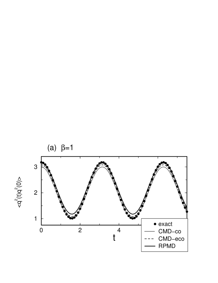
Figure 1: The plot of the exact canonical correlation function Eq. (31), the CMD correlation function with the classical operator (CMD-co) Eq. (32), the CMD correlation function with the effective classical operator (CMD-eco) Eq. (33), and the RPMD correlation function Eq. (34) for the quantum harmonic oscillator (28). (a) at $\beta=1$ and (b) at $\beta=10$.

Figure 1 shows the plot of the four correlation functions, Eqs. (31)-(34), at two different temperatures with the parameters $\hbar=k_{B}=m=\omega=1$. Here we have also set $P$ as $1000$, which is so large as to make the RPMD results converged sufficiently. At higher temperature $\beta=1$, in Fig. 1 (a), all the CMD results and the RPMD result are slightly deviate from the exact one. These deviations become remarkable at lower temperature $\beta=10$ [Fig. 1 (b)]. As is observed clearly at $\beta=10$, the CMD correlation functions [Eqs. (32) and (33)] fail to reproduce the exact value at $t=0$ and the exact amplitude, while they oscillate with the correct frequency $2\omega$. On the other hand, the RPMD correlation function (34) is exact at $t=0$, while it damps with time because of the dephasing effect caused by the mode summation $\sum_{n=1}^{P}$. This damping is remarkable at lower temperature.

For the CMD method, Jang and Voth have explicitly shown that the CMD should be used for the computation of the canonical correlation function $\langle\hat{A}(t)\hat{B}(0)\rangle_{\beta}^{\rm can}=(1/\beta)\int_{0}^{\beta}d\lambda~{}\langle\hat{A}(t-i\hbar\lambda)\hat{B}(0)\rangle_{\beta}$ where the operator $\hat{A}$ must be linear in position and/or momentum operators jv . As for the operator $\hat{B}$, the effective classical operator $B_{\beta}^{c}$ should be used for the CMD description of this correlation function jv . The CMD method is known to be problematic when the operator $\hat{A}$ is a nonlinear function. Afterwards two major approaches have been reported to deal with this nonlinear operator problem in the CMD method reich ; geva1 . Here we note these approaches:

(1) The first approach is a theory based on the higher-order Kubo-transformed correlation function; Reichman et al. have pointed out that the CMD correlation function with the effective classical operator $B_{\beta}^{c}$, $\langle q^{n}_{c}(t)B^{c}_{\beta}(0)\rangle_{\beta}^{\rm CMD}$, corresponds to the $n$th-order Kubo-transformed correlation function $\langle\hat{q}^{n}(t)\hat{B}(0)\rangle_{\beta}^{n{\rm th}}$ reich . That is, the CMD correlation function with effective classical operator, $\langle q^{2}_{c}(t)(q^{2})^{c}_{\beta}(0)\rangle_{\beta}^{\rm CMD}$, corresponds to the second-order Kubo-transformed correlation function

$$\langle\hat{q}^{2}(t)\hat{q}^{2}(0)\rangle_{\beta}^{\rm 2nd}=\frac{2}{\beta^{2}}\int_{0}^{\beta}d\lambda\int_{0}^{\beta}d\eta~{}\langle\hat{q}(t-i\hbar\lambda)\hat{q}(t-i\hbar\eta)\hat{q}^{2}(0)\rangle_{\beta}.$$ (35)

For the harmonic oscillator (28), it can readily be shown that Eq. (33) is equal to Eq. (35). Thus, the CMD with effective classical operators works very well in this framework. However, there remains a practical problem in converting the higher-order Kubo-transformed correlation function $\langle\hat{q}^{n}(t)\hat{B}(0)\rangle_{\beta}^{n{\rm th}}$ to the original quantum correlation function $\langle\hat{q}^{n}(t)\hat{B}(0)\rangle_{\beta}$; this conversion would be a complicated procedure in general.reich

(2) The second approach is based on novel expressions for physical quantities, which are formulated using correlation functions involving linear operators. Geva et al. have shown that the quantum reaction rate constant can be expressed in terms of the canonical correlation function $\langle\hat{q}(t)\hat{B}(0)\rangle_{\beta}^{\rm can}$ geva1 . Their approach enables us to evaluate the rate constants via CMD calculations without further approximations geva1 ; geva2 .

IV NUMERICAL TESTS : AN ANHARMONIC SYSTEM

In this section we calculate the EPAC correlation function $\langle\hat{q}^{2}(t)\hat{q}^{2}(0)\rangle_{\beta}^{\rm EPAC}$ for an asymmetric anharmonic system with the classical potential cv ; cm ; hk2 ; jv ; reich

$$V(q)=\frac{1}{2}~{}\!q^{2}+\frac{1}{10}~{}\!q^{3}+\frac{1}{100}~{}\!q^{4},$$ (36)

where natural units $\hbar=k_{B}=m=1$ are employed. In the following, first we show the calculated EPAC correlation functions with the exact correlation functions $\langle\hat{q}^{2}(t)\hat{q}^{2}(0)\rangle_{\beta}$, and then we present a simplified version of the EPAC method to discuss its validity.

IV.1 EPAC results for an anharmonic oscillator

To evaluate the standard effective potential $V_{\beta}(Q)$, we need to compute the generating functional $W_{\beta}[J]$ [Eq. (3)] and to carry out the Legendre transformation (5). There are various computational schemes to evaluate the generating functional $W_{\beta}[J]$. Among them, the PIMD/PIMC technique is a practical tool to evaluate $W_{\beta}[J]$ directly or indirectly hk1 ; hk2 ; owy . Here we have, however, employed the renormalization group (RG) method, which is suitable for precise calculation of $W_{\beta}[J]$ drg . Then the standard effective potential $V_{\beta}(Q)$ has been computed by means of the numerical Legendre transformation owy . Figure 2 shows the evaluated standard effective potentials at various inverse temperatures $\beta=$ 0.1, 1, 10, and 100. Minimizing the effective potential $V_{\beta}(Q)$, we have obtained the quantities $Q_{\rm min}$, $\omega_{\beta}$, $a_{3}$, and $a_{4}$. Table 1 lists the results of computed quantities for the system (36).

Table 1: The results of the quantities for the quantum anharmonic oscillator (36).

$\beta$	$Q_{\rm min}$	$\omega_{\beta}$	$a_{3}$	$a_{4}$
0.1	-1.3735019	1.07083695	0.10132291	0.1018375
1	-0.3375973	0.91069063	0.41549732	0.3305302
10	-0.1501482	0.96628105	0.54407872	0.2606658
100	-0.1501276	0.96631313	0.54396628	0.2608735

Then we have obtained the EPAC correlation function $\langle\hat{q}^{2}(t)\hat{q}^{2}(0)\rangle_{\beta}^{\rm EPAC}$ using the quantities listed in Table 1. For reference, we have also calculated the exact quantum correlation function $\langle\hat{q}^{2}(t)\hat{q}^{2}(0)\rangle_{\beta}$ by solving the Schrödinger equation numerically sch . Figure 3 shows the real part of $\langle\hat{q}^{2}(t)\hat{q}^{2}(0)\rangle_{\beta}^{\rm EPAC}$ together with the real part of $\langle\hat{q}^{2}(t)\hat{q}^{2}(0)\rangle_{\beta}$ at various inverse temperatures $\beta=$ 0.1, 1, and 10. At $t=0$, each EPAC correlation function is in very good agreement with the exact correlation function. This means that the LPA [Eq. (14)], which is the only approximation employed in the EPAC method, is fairly good for the calculation of the static property $\langle\hat{q}^{2}(0)\hat{q}^{2}(0)\rangle_{\beta}$. In fact, good results have also been obtained in the calculation of the EPAC correlation function involving the linear operator $\hat{q}$, $\langle\hat{q}(0)\hat{q}(0)\rangle_{\beta}^{\rm EPAC}$, for the system (36) hk2 .

On the other hand, as time $t$ increases, each EPAC correlation function deviates from the exact one and this deviation becomes worse at higher temperature. There are a couple of reasons for such deviation. The first is the number of oscillation modes in the correlation functions. Although the EPAC correlation function (23) consists of a limited number of oscillation modes with the frequencies $\omega_{\beta}$, $2\omega_{\beta}$, and $3\omega_{\beta}$, the exact correlation function $\langle\hat{q}^{2}(t)\hat{q}^{2}(0)\rangle_{\beta}$, in general, consists of many oscillation modes. Then at higher-temperature $\beta=0.1$ [Fig. 3 (a)], a larger number of oscillation modes get to contribute to the exact correlation function, resulting in rapid damping. The EPAC correlation function $\langle\hat{q}^{2}(t)\hat{q}^{2}(0)\rangle_{\beta}^{\rm EPAC}$ including only three oscillation modes cannot represent such damping behavior. On the other hand, as the temperature lowers [Fig. 3 (b) and (c)], the EPAC correlation function becomes very closer to the exact one because oscillation modes involved in the exact correlation function become fewer. This is the same behavior as we observed in the calculation of $\langle\hat{q}(t)\hat{q}(0)\rangle_{\beta}^{\rm EPAC}$ for the system (36) hk2 . The second reason for the disagreement between the EPAC and the exact results at long time is found in the anomalous terms in the EPAC correlation function (23). In Eq. (23), the components $A(t)$ and $B(t)$ both contain the terms proportional to $t\sin 2\omega_{\beta}t$ or $t\cos 2\omega_{\beta}t$, which exhibit amplified oscillations and diverge in the long time limit. It is expected that these anomalous terms disappear only if we calculate the higher order derivative terms in the effective action $\Gamma_{\beta}[Q]$ beyond the LPA [Eq. (14)]. A divergence-free EPAC correlation function could also be obtained if we omitted all the terms proportional to $\tau e^{-2\omega_{\beta}\tau}$ or $\tau e^{2\omega_{\beta}\tau}$ in Eq. (22). However, it should be noted that such prescription would break the periodicity of the imaginary time Green function, $\langle T\hat{q}^{2}(\beta\hbar)\hat{q}^{2}(0)\rangle_{\beta}=\langle T\hat{q}^{2}(0)\hat{q}^{2}(0)\rangle_{\beta}$.

Finally we mention how the EPAC method could capture the anharmonic effects in quantum statistical systems. In the EPAC method, all the quantum/thermal effects are included via the standard effective potential $V_{\beta}(Q)$. For the harmonic case (28), the effective frequency equals the classical frequency ($\omega_{\rm eff}=\omega$), and the higher-order coefficients vanish ($a_{n}=0$ for $n\geq 3$). However, for anharmonic systems, the effective frequency $\omega_{\rm eff}$ deviates from the classical one and the higher-order coefficients $a_{n\geq 3}$ have nonzero values. As seen in Eq. (23), the coefficients $a_{n\geq 3}$ contribute only to the amplitude of the oscillations of the EPAC correlation functions, while the effective frequency $\omega_{\rm eff}$ provides oscillation modes with the frequency $l\omega_{\beta}$ ($l$: integer). The EPAC is a method to approximate the exact dynamics of quantum systems using a finite number of oscillation modes with the frequency $l\omega_{\beta}$, and therefore the EPAC correlation function always exhibits harmoniclike oscillations. That is, although the anharmonic effects are included via the quantities $\omega_{\rm eff}$ and $a_{n\geq 3}$, the EPAC correlation functions cannot reproduce a certain type of anharmonic effects such as the dephasing and the rapid damping at higher temperature [Fig. 3 (a)]. This quasiharmonic property of the EPAC correlation function comes from the LPA [Eq. (14)], the only approximation employed in the EPAC method. At the same time, we should note an important problem arising in the standard effective potential approach when it is applied to quantum systems that include the dissociation limit $\lim_{|\bm{q}|\to\infty}V(\bm{q})=0$ hk2 ; ct ; for example, the systems represented in terms of the Morse potential $V(r)~{}(r=|\bm{q}_{1}-\bm{q}_{2}|)$ are classified into this category. For such systems with the dissociation limit, the minimum should disappear in the standard effective potential $V_{\beta}(R)$ because it is always convex for $0<R<\infty$ according to its definition riv ; ps ; hk1 . Then the frequency $\omega_{\beta}$ cannot be defined; this would lead to some unphysical flaw. Therefore, the EPAC is not very suitable for the full description of, e.g., the dissociation reaction of isolated diatomic molecules. Still we note that at low temperatures the EPAC does work well because the polynomial expansion around the potential minimum $r_{\rm min}$ is so valid as to neglect the dissociation limit approximately hk2 .

As for quantum liquids whose intermolecular interaction is represented in terms of, e.g., the Lennard-Jones potential with the dissociation limit as well, the situation of such many-body systems is not so simple as an isolated diatomic system, because potential-energy surface in configurational space includes many local minima sw ; zw . Reichman and Voth have discussed various effective harmonic theories for liquid dynamics associated with the curvature of such potential-energy surface rv . Certainly, there is a similarity between the effective harmonic theories for liquids and the standard effective potential approach we are discussing, in that $\omega_{\beta}$ is defined as the second derivative of the standard effective potential $V_{\beta}(Q)$ as well. However, the standard effective potential and the derived EPAC method is not suitable for describing the diffusion in liquids because some well-defined multidimensional $V_{\beta}(\bm{Q})$ should be convex to have a single minimum for one-dimension, resulting in just the oscillatory motions with real positive frequencies $\omega_{\beta}^{(i)}$. Thus, at the present stage, the EPAC method does not fully capture the molecular diffusion in quantum liquids bLPA .

Rather, the EPAC method should be useful for the investigation of, e.g., the coherent dynamics in bound systems involving proton transfer reaction proton for which the model potentials are typically represented as double-well type such as $V(q)=-aq^{2}+bq^{4}~{}(a,b>0)$. These potentials are asymptotically superlinear, $\lim_{|\bm{q}|\to\infty}V(\bm{q})/|\bm{q}|>0$, without dissociation limit. In such potential systems the quasioscillating behavior of a correlation function is essential. It is true that this oscillation is a consequence of the quantum coherence between the localized states in the local minima of $V(\bm{q})$. The EPAC method based on $V_{\beta}(\bm{Q})$ is suitable for describing such oscillation hk1 , because its frequencies $\omega_{\beta}^{(i)}$ are evaluated from the convex effective potential $V_{\beta}(\bm{Q})$, which includes the effects of quantum interference between the localized states riv ; owy .

IV.2 Truncated EPAC method

In this subsection we present a further approximation scheme useful for practical computation. Here we treat the truncated expansion of $V_{\beta}$ around the minimum $Q=Q_{\rm min}$,

$$V_{\beta}(Q)=\sum_{n=0}^{2}\frac{a_{n}}{n!}(Q-Q_{\rm min})^{n}.$$ (37)

This means that we approximate the standard effective potential $V_{\beta}$ as an effective harmonic potential and omit all the higher order derivatives of $V_{\beta}(Q)$, $a_{n}=\partial^{n}V_{\beta}/\partial Q^{n}|_{Q=Q_{\rm min}}~{}(n\geq 3)$. Since the determination of $a_{n\geq 3}$ requires a heavy computation of $V_{\beta}(Q)$ with high precision, the truncation such as Eq. (37) reduces the computational cost significantly.

Using Eq. (37), we obtain the truncated EPAC correlation function

$$\langle\hat{q}^{2}(t)\hat{q}^{2}(0)\rangle_{\beta}^{tEPAC}=D(t),$$ (38)

where $D(t)$ is just the function given in Eq. (27). This is the completely harmonic version of the EPAC method. Figure 4 shows the real part of Eq. (38) together with the real part of the exact quantum correlation function for the quantum anharmonic oscillator (36). The temperatures are the same as in Fig. 3. Here we have used again the results of $Q_{\rm min}$ and $\omega_{\beta}$ listed in Table 1.

We see that, at $t=0$, the truncated EPAC correlation functions are in good agreement with the exact results except for the middle temperature $\beta=1$ [Fig. 4 (b)]. This behavior can be explained qualitatively as follows. Since $\coth\alpha\geq 1$, the highest power of $\coth\alpha$ is regarded as the dominating factor in each term in the full EPAC correlation function (23) at $t=0$,

$$a_{4}A(0) \sim -\frac{1}{32}\frac{a_{4}}{\omega_{\beta}^{5}}\coth^{3}\alpha,$$ (39)

$$a_{3}^{2}B(0) \sim \frac{5}{96}\frac{a_{3}^{2}}{\omega_{\beta}^{7}}\coth^{5}\alpha,$$ (40)

$$a_{3}Q_{\rm min}C(0) \sim -\frac{1}{3}\frac{a_{3}Q_{\rm min}}{\omega_{\beta}^{4}}\coth^{2}\alpha,$$ (41)

$$D(0) \sim \frac{3}{4}\frac{1}{\omega_{\beta}^{2}}\coth^{2}\alpha,$$ (42)

where $\omega_{\beta}\sim{\it O}(1)$ (see Table 1). For lower temperature $\beta=10$, since $\coth\alpha\simeq 1$ and $a_{3},a_{4}<1$ (see Table 1), all the anharmonic terms in Eq. (23) at $t=0$, i.e., $a_{4}A(0)$, $a_{3}^{2}B(0)$, and $a_{3}Q_{\rm min}C(0)$, become negligible. Therefore the truncated EPAC result at $t=0$, $\langle\hat{q}^{2}(0)\hat{q}^{2}(0)\rangle_{\beta}^{\rm tEPAC}$ [Eq. (38)], is a good approximation to the full EPAC result. On the other hand, as the temperature increases, $\coth\alpha$ becomes larger than unity, and then the anharmonic terms $a_{4}A(0)$ and $a_{3}^{2}B(0)$ are no longer negligible in the full EPAC correlation function (23), because they contain $\coth^{3}\alpha$ and $\coth^{5}\alpha$, respectively. Thus the truncated EPAC correlation function without the anharmonic terms fails to reproduce the full EPAC result at the middle temperature $\beta=1$ [Fig. 4 (b)]. However, for higher-temperature $\beta=0.1$, the coefficients $a_{3}$ and $a_{4}$ become very small and therefore the standard effective potential $V_{\beta}(Q)$ has an effectively harmonic shape. Consequently, the truncation such as Eq. (37) becomes a very good approximation to the full potential (18), and therefore the truncated EPAC can reproduce the full EPAC result very well again.

As for the long time behavior, a discussion can be made as follows. The truncated EPAC correlation function $\langle\hat{q}^{2}(t)\hat{q}^{2}(0)\rangle_{\beta}^{\rm tEPAC}$ consists of two oscillation modes with the frequencies $\omega_{\beta}$ and $2\omega_{\beta}$, and it lacks the oscillation mode with frequency $3\omega_{\beta}$ which exists in the full EPAC correlation function $\langle\hat{q}^{2}(t)\hat{q}^{2}(0)\rangle_{\beta}^{\rm EPAC}$. Nevertheless, the truncated EPAC correlation function correctly reproduces the oscillation appearing in the full EPAC correlation function at each temperature (Figs. 3 and 4). This is because the oscillation mode with frequency $3\omega_{\beta}$ exists only in $B(t)$ and its contribution to Eq. (23) is relatively small. It should also be noted that the truncated EPAC correlation function, only $D(t)$, is free from an amplified oscillation expected in Eq. (23) and it never diverges in the $t\to\infty$ limit. We therefore expect that the truncated EPAC method, Eq. (38), works well in low-temperature systems. Thus the truncated EPAC method can be useful for the practical calculation of the nonlinear dynamical properties of low-temperature condensed phase systems because it should reduce the computational cost.

V CONCLUDING REMARKS

In this paper, we have focused on the nonlinear operator problem in quantum dynamics methods. At first, we have shown how to apply the EPAC method to the calculation of the correlation function $\langle\hat{q}^{n}(t)\hat{q}^{n}(0)\rangle_{\beta}$ and have given the EPAC correlation function $\langle\hat{q}^{2}(t)\hat{q}^{2}(0)\rangle_{\beta}^{\rm EPAC}$ as an example. It has been shown that the EPAC method is exact in a harmonic system, while the other quantum dynamics methods, the CMD and the RPMD, fail to reproduce the exact results even in the harmonic system.

Then we have applied the EPAC method to the asymmetric anharmonic system. We have seen that the EPAC correlation function at $t=0$ agrees well with the exact correlation function $\langle\hat{q}^{2}(0)\hat{q}^{2}(0)\rangle_{\beta}$. As for the long time behavior, the EPAC result becomes better at lower temperature. These good properties suggest that the EPAC method can be a useful quantum dynamics method for nonlinear correlation functions of low temperature systems. We have also seen that the EPAC correlation function contains the terms which cause amplified oscillation. We suppose that these anomalous terms would disappear only if we improved the approximation beyond the LPA.

Finally we have discussed the truncated EPAC method which is given by the truncation of the standard effective potential $V_{\beta}(Q)$. We have tested this method in the same anharmonic system to which the full EPAC method has also been applied. Although the truncated EPAC method is not so good as the full EPAC method, it works fine at lower temperature. Since the truncated EPAC needs only the information up to the second order derivative of the standard effective potential $V_{\beta}(Q)$, it should significantly reduce the computational cost. Therefore, from a practical aspect, we expect that the truncated EPAC is more suitable than the full EPAC for complex many-body systems at lower temperature.

In the present work, the discussions have been restricted in the evaluation of the correlation function $\langle\hat{q}^{n}(t)\hat{q}^{n}(0)\rangle_{\beta}$. However, the multitime quantum correlation functions, e.g., $\langle\hat{q}(t_{1})\hat{q}(t_{2})\hat{q}(t_{3})\hat{q}(0)\rangle_{\beta}$, are also important property especially in the context of the nonlinear optical spectroscopy mukamel . It is a challenging task to apply the EPAC method to such calculation of multitime quantum correlation functions in near future.

Figure 2: The inverse temperature $\beta$-dependence of the standard effective potential $V_{\beta}(Q)$ for the asymmetric anharmonic classical potential (36). In this plot we set $V_{\beta}(Q_{\rm min})=0$.

Figure 3: The plot of the real part of the exact quantum correlation function $\langle\hat{q}^{2}(t)\hat{q}^{2}(0)\rangle_{\beta}$ and the real part of the EPAC correlation function $\langle\hat{q}^{2}(t)\hat{q}^{2}(0)\rangle_{\beta}^{\rm EPAC}$ for the quantum anharmonic oscillator (36). (a) at $\beta=0.1$, (b) at $\beta=1$, and (c) at $\beta=10$.

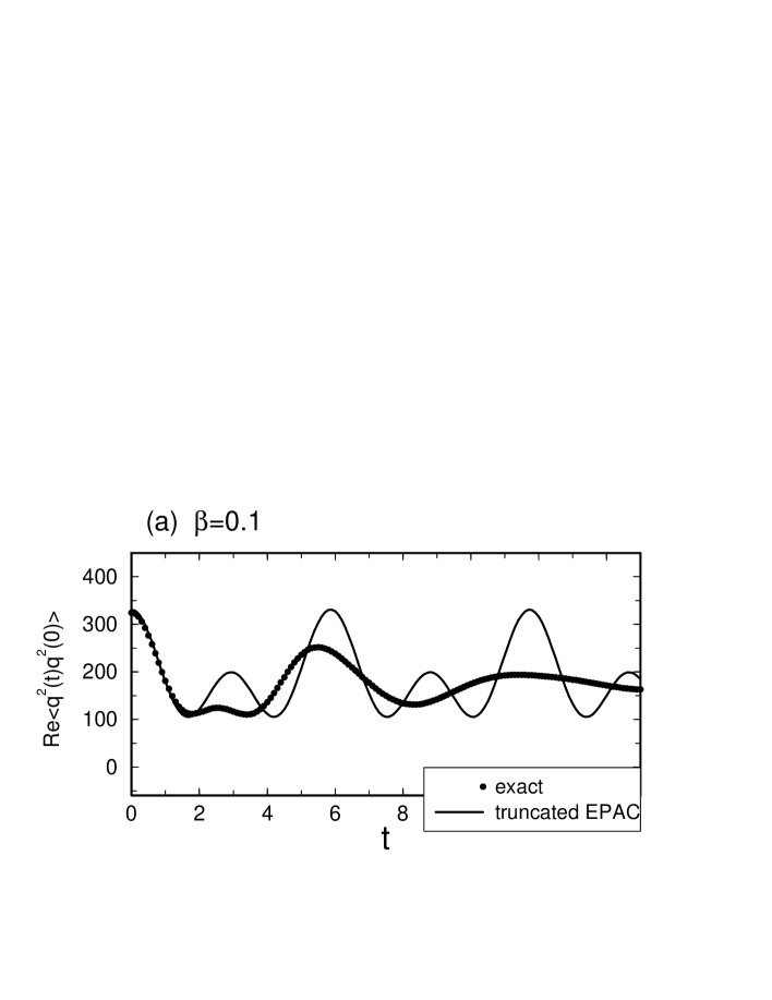
Figure 4: The plot of the real part of the exact quantum correlation function $\langle\hat{q}^{2}(t)\hat{q}^{2}(0)\rangle_{\beta}$ and the real part of the truncated EPAC correlation function $\langle\hat{q}^{2}(t)\hat{q}^{2}(0)\rangle_{\beta}^{\rm tEPAC}$ for the quantum anharmonic oscillator (36). (a) at $\beta=0.1$, (b) at $\beta=1$, and (c) at $\beta=10$.