Increasing identical particle entanglement by fuzzy measurements

Abstract

We investigate the effects of fuzzy measurements on spin entanglement for identical particles, both fermions and bosons. We first consider an ideal measurement apparatus and define operators that detect the symmetry of the spatial and spin part of the density matrix as a function of particle distance. Then, moving on to realistic devices that can only detect the position of the particle to within a certain spread, it was surprisingly found that the entanglement between particles increases with the broadening of detection.

Entanglement is one of the most studied subjects in contemporary physics. This quantum mechanical property is the core of a whole new area in physics, mathematics and computation, known as quantum information theory. It has also been perceived as a useful resource for different technological applications nielsen . However much has still to be done in order to completely understand these non-classical correlations. One of the important aspects that still deserves further investigation concerns the actual observation of entanglement due to the indistinguishable character of the quantum world.

Usually, when talking about entanglement, one tends to ignore the role of the measurement apparatus, always considering ideal situations. However, there is no such a thing as an ideal detector, and the detector bandwidth affects the measurement of entanglement. Furthermore, in the particular case of identical particles, it is still not clear how the symmetry of detection in external degrees of freedom affects the entanglement of the internal ones.

In this paper we analyze these questions in two different systems: a gas of non-interacting fermions at zero temperature and a photonic interferometer. In particular, we analyze how the measurement of external degrees of freedom can affect the entanglement in internal degrees of freedom in a system of identical particles. First, we show how the symmetry of detection affects the entanglement of two fermions detected in a non-interacting fermion gas at zero temperature. Then, we study how imperfect detections affect the observation of entanglement both for the fermionic gas and also for an interferometer of photons.

Recently Vedral showed that the entanglement between two particles in a non-interacting Fermi gas at zero temperature decreases with increasing distance from each other vedral . Vedral also shows that there is a limit below which any two fermions extracted from the gas are certainly entangled. In particular, if both fermions are extracted at the same position, then the Pauli exclusion principle forces their spin to be maximally entangled in a typical antisymmetric Bell state.

In order to calculate the upper limit for guaranteed entanglement, the author used the Peres-Horodecki criterion peres , which in his paper, corresponds to $f^{2}>\frac{1}{2}$, where $f(r-r^{\prime})=3j_{1}(k_{F}|r-r^{\prime}|)/(k_{F}|r-r^{\prime}|)$, $|r-r^{\prime}|$ is the distance between the fermions, $p_{f}=\hbar k_{F}$ is the Fermi momentum and $j_{1}$ is a spherical Bessel function. In order to obtain this result, the author defines (apart from normalization) the spin density matrix of these two particles from the second order correlation function (see the Appendix for a justification)

$$\rho^{(2)}_{ss^{\prime},tt^{\prime}}=\left\langle\Phi_{0}\right|\Psi^{\dagger}_{t^{\prime}}(r^{\prime})\Psi^{\dagger}_{t}(r)\Psi_{s^{\prime}}(r^{\prime})\Psi_{s}(r)\left|\Phi_{0}\right\rangle,$$ (1)

which corresponds to measuring these two fermions at positions $r$ and $r^{\prime}$ (the subscriptions $s$,$s^{\prime}$, $t$, and $t^{\prime}$ refer to the spin of the particles). The initial state $|\phi_{0}\rangle$ is the ground state of the Fermi system

$$\left|\phi_{0}\right\rangle=\Pi_{s,p}b_{s}^{\dagger}(p)\left|0\right\rangle,$$ (2)

and the detection operator at position $r$ and spin $s$ is given by,

$$\Psi_{s}^{\dagger}(r)=\int_{0}^{p_{f}}\frac{d^{3}p}{(2\pi)^{3}}e^{-ipr}b_{s}^{\dagger}(p).$$ (3)

A typical interpretation of this result is related to the spatial overlap of the wavefunctions of each fermion.

Here, we present a clearer and more complete explanation to this behavior through the analysis of the symmetry of the position detection. To do so let us define new detection operators:

$$\Pi^{+}_{ss^{\prime}}(r,r^{\prime}) \equiv \frac{\left(\Psi_{s}(r)\Psi_{s^{\prime}}(r^{\prime})+\Psi_{s^{\prime}}(r)\Psi_{s}(r^{\prime})\right)}{\sqrt{2}},$$ (4a)

$$\Pi^{-}_{ss^{\prime}}(r,r^{\prime}) \equiv \frac{\left(\Psi_{s}(r)\Psi_{s^{\prime}}(r^{\prime})-\Psi_{s^{\prime}}(r)\Psi_{s}(r^{\prime})\right)}{\sqrt{2}}.$$ (4b)

The operator $\Pi^{+}_{ss^{\prime}}(\Pi^{-}_{ss^{\prime}})$, detects the antisymmetric (symmetric) spatial part and the symmetric (antisymmetric) spin part of fermion wavefunction.

In terms of these new operators, Eq.(1) becomes:

$$\rho_{ss^{\prime},tt^{\prime}}^{(2)}=\frac{1}{2}\langle\Phi_{0}|[\Pi^{+\dagger}_{tt^{\prime}}(r,r^{\prime})+\Pi^{-\dagger}_{tt^{\prime}}(r,r^{\prime})][\Pi^{+}_{ss^{\prime}}(r,r^{\prime})+\Pi^{-}_{ss^{\prime}}(r,r^{\prime})]|\Phi_{0}\rangle$$ (5)

Note that written in this way, the two-fermion density matrix is the sum of four different terms, two of which contain only symmetric and antisymmetric spin detectors. The other two are the crossing terms, which vanish due to the exclusion principle (spin and position of two fermions cannot be both symmetric or antisymmetric). The remaining terms are:

$$\rho_{sym} = \frac{1}{2}\left\langle\Phi_{0}\right|\Pi^{+\dagger}_{tt^{\prime}}(r,r^{\prime})\Pi^{+}_{ss^{\prime}}(r,r^{\prime})\left|\Phi_{0}\right\rangle,$$ (6a)

$$\rho_{asym} = \frac{1}{2}\left\langle\Phi_{0}\right|\Pi^{-\dagger}_{tt^{\prime}}(r,r^{\prime})\Pi^{-}_{ss^{\prime}}(r,r^{\prime})\left|\Phi_{0}\right\rangle.$$ (6b)

Here $\rho_{sym}$ takes into consideration only the symmetric spin function (therefore, it is related to the detection of the antisymmetric part of the spatial wavefunction) while $\rho_{asym}$ contains only the antisymmetric spin function (therefore related to the detection of the symmetric part of the spatial wavefunction). The density matrix can be rewritten as:

$$\rho^{(2)} = \rho_{asym}+\rho_{sym}$$ (11)

$$= \int\!\!\!\!\int dpdp^{\prime}\frac{1}{2}\left\{(1+e^{i(p-p^{\prime})(r-r^{\prime})})\left(\begin{array}[]{cccc}&&&\\ &1&-1&\\ &-1&1&\\ &&&\end{array}\right)\right.$$

$$+ \left.(1-e^{i(p-p^{\prime})(r-r^{\prime})})\left(\begin{array}[]{cccc}2&&&\\ &1&1&\\ &1&1&\\ &&&2\end{array}\right)\right\}.$$ (16)

First, note that, as expected, for $r=r^{\prime}$, the antisymmetric spatial function goes to zero, and the spin wavefunction has to be antisymmetric (first term in Eq.(16)). For $r-r^{\prime}\neq 0$ both parts contribute. Note, however, that the symmetric spin density matrix can be viewed as an equal weight mixture of the three triplet components, and has no entanglement at all (by the Peres-Horodecki criterion). The spin state in Eq.(16) represents a convex combination of singlet state and the equal mixture of triplet states. It will have entanglement iff the fraction of singlet is sufficiently larger than the fraction of triplets, in a similar context to the calculation of relative robustness robust . In the limit $r-r^{\prime}\gg 1/k_{F}$, as the integrals on Eq.(16) are performed over momenta below the (momentum equivalent of) Fermi surface the momentum dependent terms oscillate too fast, and average to zero. Therefore, the spin density matrix becomes just the identity ($\delta_{ts}\delta_{t^{\prime}s^{\prime}}$). This behavior can be seen as a smooth transition from a quantum statistics (Fermi-Dirac) to a classical one (Maxwell-Boltzmann).

Another way of analyzing Eq.(16) is given in Ref.ohkim , where the authors describe $\rho^{(2)}$ as a Werner state. Here, it becomes clear how the symmetry of the spatial detection is influencing the behavior of the spins, and also why there is no entanglement from $|r-r^{\prime}|\sim 1/k_{F}$ on.

An interesting question arises when considering non-punctual (non-ideal) position detections, i.e. more realistic apparatus that detect the position of those fermions with some uncertain. Instead of Eq.(3), the detection operator should be written as the general field operator:

$$\Psi_{s}(r)=\int\!\!\!\!\int e^{ipr^{\prime\prime}}D(r-r^{\prime\prime})b_{s}(p)dr^{\prime\prime}dp.$$ (17)

The perfect position measurement situation is the particular case of Eq.(17) corresponding to $D(r-r^{\prime\prime})=\delta(r-r^{\prime\prime})$. However, if $D(r-r^{\prime\prime})$ has some position uncertainty, like, for example, if it is described by a gaussian with spread $\sigma$,

$$D(r-r^{\prime\prime})=\frac{1}{\sqrt{2\pi}\sigma}e^{\frac{-|r-r^{\prime\prime}|^{2}}{2\sigma^{2}}},$$ (18)

then, the field operators become

$$\Psi_{s}(r)=\frac{1}{\sqrt{2\pi}\sigma}\int\!\!\!\!\int e^{ipr^{\prime\prime}}e^{\frac{-|r-r^{\prime\prime}|^{2}}{2\sigma^{2}}}b_{s}(p)dr^{\prime\prime}dp.$$ (19)

These operators, when substituted back in Eq.(1), give:

$$\rho_{ss^{\prime},tt^{\prime}} = \delta_{st}\delta_{s^{\prime}t^{\prime}}f(d,\sigma)+\delta_{st^{\prime}}\delta_{s^{\prime}t}g(d,\sigma),$$ (20a)

with $$d=|r-r^{\prime}|$$,

$$f(d,\sigma)=\left(\frac{\mathrm{erf}(\sigma p_{f})}{\sigma}\right)^{2},$$ (20b)

$$g(d,\sigma) = \frac{1}{\sigma^{2}}e^{\frac{-d^{2}}{2\sigma^{2}}}\{\mathrm{erf}(\sigma p_{f}-\frac{id}{2\sigma})-\mathrm{erf}(-\frac{id}{2\sigma})\}$$ (20c)

$$\times \{\mathrm{erf}(\sigma p_{f}+\frac{id}{2\sigma})-\mathrm{erf}(\frac{id}{2\sigma})\},$$

and $$\mathrm{erf}(x)$$ is the “error function”, defined via:

$$erf(x)\equiv\frac{2}{\sqrt{\pi}}\int_{0}^{x}exp(-t^{2})dt.$$ (20d)

In order to make clearer the behavior of entanglement in relation to changes in $d$ and $\sigma$ we can compute the negativity ($\mathcal{N}$) negativity of the state $\rho^{(2)}(d,\sigma,p_{f})$. This entanglement quantifier was chosen because it is an entanglement monotone monot (i.e.: satisfies all the required features of a good entanglement quantifier), and also it is easy to calculate. $\mathcal{N}(\rho)$ is equal to twice the absolute value of the negative eigenvalue of the partial transpose of $\rho$, $\rho^{T_{A}}$. $\mathcal{N}(\rho)$ measures by how much $\rho^{T_{A}}$ fails to be positive semi-definite negativity . In our case $\mathcal{N}(\rho)$ reads as

$$\mathcal{N}(\rho)=2\mu(\frac{f-2g}{4f-2g})$$ (21)

where $\begin{array}[]{c}\mu=\left\{\begin{array}[]{rl}-x\ ,&x<0\\ 0\ ,&x\geq 0\end{array}\right.\end{array}$. This function is plotted in Fig. 1 for some values of $\sigma$.

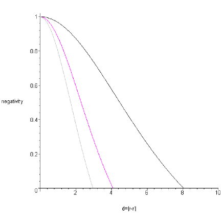
Figure 1: (Color online) $\mathcal{N}(\rho)$ vs. $d$ for $p_{f}=1$ and $\sigma=1$ (grey), $\sigma=2$ (magenta) and $\sigma=4$ (black).

Note that, for imperfect position detection, the entanglement decreases as the detectors become apart from each other, but increases if the spread in the detection becomes larger. The fact that inaccuracy in the detection increases entanglement seems surprising. However it has to be noted that as our knowledge in position gets worst, our knowledge in momentum gets better. In the limit of infinite spread, both detectors become perfect momentum detectors (centered at $p=0$, see Eq.(18)), which means again that their spin wavefunction should be totally antisymmetrized, hence they are found in the antisymmetric Bell state. It is important to stress that Eq.(17) describes a coherent combination of localized field operators instead of a statistical average of them. That is the reason for the infinite spread limit be a momentum-localized detector instead of just a vague “there is a particle somewhere”.

A similar situation can be found in a bosonic system calculating the entanglement in polarization between photons placed in an interferometer using polarization beam splitters (PBS). In this analysis the polarization and frequency of the photons play the role of the spin and momentum of the fermionic case. This kind of interferometry has been extensively studied in practical experiments hongoumandel and thus, in principle, the results presented here could be tested experimentally.

First we write the modes after the PBS if the modes before it are $a_{1,\epsilon}$ and $a_{2,\epsilon}$ (see Fig.2):

$$E_{3,\epsilon}(\omega) = T_{\epsilon}a_{1,\epsilon}(\omega)+i{R_{\epsilon}}a_{2,\epsilon}(\omega)e^{i\omega\tau},$$ (22a)

$$E_{4,\epsilon}(\omega) = iR_{\epsilon}a_{1,\epsilon}(\omega)+T_{\epsilon}^{*}a_{2,\epsilon}(\omega)e^{i\omega\tau},$$ (22b)

with $|T_{\epsilon}|^{2}$ and $|R_{\epsilon}|^{2}$ being the transmissivity and reflectivity of the $\epsilon$ polarization in the PBS, $\tau=\tau_{1}-\tau_{2}$, where $\tau_{1}$ and $\tau_{2}$ are the propagation times from the crystal to the detectors via path 1 and path 2 respectively.

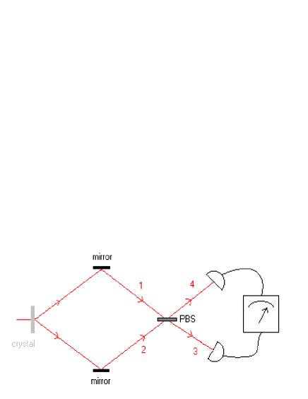
Figure 2: (Color online) Hong-Ou-Mandel type of interferometer.

The two particle density matrix is again defined through the second-order correlation function:

$$\rho_{\epsilon{\epsilon}^{\prime},ss^{\prime}} = \int\!\!\!\!\int d\omega_{1}d\omega_{2}D(\omega_{1},\omega_{2})$$

$$\times\left\langle\phi_{0}\right|E_{3,s}^{{\dagger}}(\omega_{1})E_{4,s^{\prime}}^{{\dagger}}(\omega_{2})E_{4,\epsilon^{\prime}}(\omega_{2})E_{3,\epsilon}(\omega_{1})\left|\phi_{0}\right\rangle.$$

The state

$$|\phi_{0}\rangle=\psi^{{\dagger}}\left|0\right\rangle$$ (24)

is prepared by the two-photon creation operator

$$\psi^{{\dagger}}=\sum_{k,k^{\prime}}\int\!\!\!\!\int a_{1,k}^{{\dagger}}(\nu_{1})a_{2,k^{\prime}}^{{\dagger}}(\nu_{2})g_{k,k^{\prime}}(\nu_{1},\nu_{2})d\nu_{1}d\nu_{2},$$ (25)

with frequency distribution $g_{k,k^{\prime}}(\nu_{1},\nu_{2})$ which is, in the more general case, polarization dependent. Note that this calculation is more general than a typical Hong-Ou-Mandel interferometer, since one is free to choose initial states by $g_{k,k^{\prime}}(\nu_{1},\nu_{2})$. In a way similar to Eq.(17), detection is represented by a function $D(\omega_{1},\omega_{2})$.

Using the commutation relation for bosons and evaluating the integrals in $d\nu_{1},d\nu_{2}$ and the summations in $k,k^{\prime}$ we find:

$$\rho_{\epsilon{\epsilon}^{\prime},s^{\prime}s} = \int\!\!\!\!\int\{T_{s^{\prime}}T_{s}^{*}T_{\epsilon^{\prime}}^{*}T_{\epsilon}g_{ss^{\prime}}^{*}(\omega_{1},\omega_{2})g_{\epsilon\epsilon^{\prime}}(\omega_{1},\omega_{2})+R_{s^{\prime}}R_{s}^{*}R_{\epsilon^{\prime}}^{*}R_{\epsilon}g_{s^{\prime}s}^{*}(\omega_{2},\omega_{1})g_{\epsilon^{\prime}\epsilon}(\omega_{2},\omega_{1})$$

$$- T_{s^{\prime}}T_{s}^{*}R_{\epsilon^{\prime}}^{*}R_{\epsilon}g_{ss^{\prime}}^{*}(\omega_{1},\omega_{2})g_{\epsilon^{\prime}\epsilon}(\omega_{2},\omega_{1})e^{i(\omega_{1}-\omega_{2})\tau}-T_{\epsilon^{\prime}}^{*}T_{\epsilon}R_{s^{\prime}}R_{s}^{*}g_{\epsilon\epsilon^{\prime}}(\omega_{1},\omega_{2})g_{s^{\prime}s}^{*}(\omega_{2},\omega_{1})e^{-i(\omega_{1}-\omega_{2})\tau}\}D(\omega_{1},\omega_{2})d\omega_{1}d\omega_{2}.$$

The PBS is an optical element which allows transmission in only one polarization (say vertical), and reflection in the other one (horizontal). The coefficients of transmissivity and reflectivity can be written as $R_{h}=T_{v}=1$ and $T_{h}=R_{v}=0$. With this, and assuming a symmetric state in polarization ($g_{ss^{\prime}}=g_{s^{\prime}s}$), the unique non-vanishing coefficients are:

$$\rho_{\epsilon\epsilon,\epsilon\epsilon} = \int\!\!\!\!\int|g_{\epsilon\epsilon}(\omega_{1},\omega_{2})|^{2}D(\omega_{1},\omega_{2})d\omega_{1}d\omega_{2},\ \ \epsilon=h,v,$$ (27a)

$$\rho_{hh,vv} = -\int\!\!\!\!\int g_{vv}^{*}(\omega_{1},\omega_{2})g_{hh}(\omega_{2},\omega_{1})e^{i(\omega_{1}-\omega_{2})}D(\omega_{1},\omega_{2})d\omega_{1}d\omega_{2}=\rho^{*}_{vv,hh}.$$ (27b)

In order to carry on the calculations, let us assume particular distributions for the functions $g(\omega_{1},\omega_{2})$ and $D(\omega_{1},\omega_{2})$. Since we are more interested in the detection properties, let us first assume that $g(\omega_{1},\omega_{2})$ is constant. Then, we assume independent gaussian detectors, which means $D(\omega_{1},\omega_{2})=D(\omega_{1})D(\omega_{2})$ and

$$D(\omega)=\frac{1}{\sqrt{2\pi}\sigma}e^{-\frac{\omega^{2}}{2\sigma^{2}}}.$$ (28)

Now, we can calculate the polarization density matrix, obtaining, up to normalization,

$$\rho_{hh,hh}=\rho_{vv,vv}=\int\!\!\!\!\int D(\omega_{1})D(\omega_{2})d\omega_{1}d\omega_{2}=1,$$ (29)

and

$$\rho_{hh,vv} = \rho^{*}_{vv,hh}=-\frac{1}{2\pi\sigma^{2}}\int\exp(-\frac{\omega_{1}^{2}}{2\sigma^{2}}+i\omega_{1}\tau)d\omega_{1}$$ (30)

$$\times\int\exp(-\frac{\omega_{2}^{2}}{2\sigma^{2}}-i\omega_{2}\tau)d\omega_{2}.$$

Evaluating these Fourier transforms of Gaussian functions we obtain

$$\rho_{hh,vv}=\rho_{vv,hh}=-\exp(-\sigma^{2}\tau^{2}).$$ (31)

The (normalized) polarization density matrix then is given by

$$\rho=\frac{1}{2}\left(\begin{array}[]{cccc}1&0&0&-f\\ 0&0&0&0\\ 0&0&0&0\\ -f&0&0&1\\ \end{array}\right),$$ (32)

where $f=\exp(-\sigma^{2}\tau^{2})$. The partial transposition of $\rho$ has always one negative eigenvalue equal to $-\frac{f}{2}$. So the Negativity of $\rho$ is $\mathcal{N}(\rho)=f=\exp(-\sigma^{2}\tau^{2})$. This result shows that as the detector becomes broader in frequencies or the time delay between the two arms of the interferometer becomes larger, the entanglement between detected photon pairs decreases. One should note that time delay gives rise to which path information, while broadening in frequencies opposes to such labeling.

Again we can see the state $\rho$ as a combination of Bell states. Interestingly, in the interferometric process described here the separation is between the states $\left|\Phi+\right\rangle$ and $\left|\Phi-\right\rangle$, in the following way:

$$\rho=\frac{(1-f)}{2}\left|\Phi+\right\rangle\left\langle\Phi+\right|+\frac{(1+f)}{2}\left|\Phi-\right\rangle\left\langle\Phi-\right|,$$ (33)

and no more between symmetric and antisymmetric states as in Equation (16).

In conclusion it was shown that the measurement apparatus plays a central role in the entanglement of identical particles. That entanglement increases because of broadening in detection can sound weird at first. However it is important to say that the detections discussed here are done in a coherent way (as in most of real cases). If we have modeled the imperfect detectors as a cluster of perfect detectors things would be different. Furthermore the relation between identical particle entanglement (i.e.: the correlations due exclusively to indistinguishability) and the entanglement generated by direct interaction among the particles is not completely understood. Despite of that the framework presented here can be, a priori, also applied for interacting particle systems and then could make this relation less obscure.

Appendix A Second order correlation functions as quantum states

In this appendix we discuss why we consider the second order normalized correlation functions (1) and (20d) as two-qubit quantum states. Mathematically speaking, any trace $1$ positive operator is a state on the space state in which it is defined. Physically, however, this seems a poor justification. Moreover, why one can consider this four-dimensional linear space as a two-qubit system and obtain conclusions about its entanglement?

To answer this questions we need to consider an interplay of two aspects of quantum theory: photodetection and post-selection. In a first quantized notation, if the electromagnetic field state is described by $\rho$ and we make a one-photon detection described by the annihilation operator ${\mathbf{a}}$, the field state after such measurement will be given by $\rho^{\prime}={\mathbf{a}}\rho{\mathbf{a}}^{\dagger}$, properly renormalized (i.e.: the conditional state). As photodetection is a destructive measurement, after the click, $\rho^{\prime}$ describes the state of the remaining photons. If, however, we have a non-destructive one-photon detector, this post-selected “detected photon” would be described by the pure Fock state $\left|1\right\rangle$ of the mode annihilated by ${\mathbf{a}}$. But what if we just have a non-destructive one-photon detector similar to the one above, except by the fact that it clicks for any one-photon superposition of two specific modes (e.g.: two polarizations of one and the same spatial mode). This situation is analogous to a degenerate spectrum projective measurement. The state of the post-selected photon will preserve the coherence which it possibly had between the two modes, being described by a linear combination like $\alpha\left|1,0\right\rangle+\beta\left|0,1\right\rangle$, or, more generally, by a density operator $\tilde{\rho}={\mathbf{P}}\rho{\mathbf{P}}$, with ${\mathbf{P}}$ the projector ${\mathbf{P}}=\left|1,0\right\rangle\left\langle 1,0\right|+\left|0,1\right\rangle\left\langle 1,0\right|$, and again properly normalized. Clearly, the state of this two-level system describes the unresolved mode combination (in the example, the polarization degree of freedom).

If we detect two spatially distinguishable photons, but each of them with unresolved polarizations, the first quantized notation becomes cumbersome, but the ideas involved are the same, and the remaining two-qubit state describes the polarization degree of freedom of this two distinguished photons.

The same reasoning, with two fermions spatially localized ar $r$ and $r^{\prime}$, but with unresolved spin, in second quantized notation, give rise to Eq.(1), that then describes the spin state of the two localized fermionsYang . In this sense, (normalized) second order correlation functions can be considered as quantum states, and its entanglement properties can be studied, as is done in this paper.

References

- (1) M.A. Nielsen and I.L. Chuang, Quantum Computation and Quantum Information,(Cambridge Univesity Press, Cambridge, UK, 2000).
- (2) V. Vedral, Cent. Eur. J. Phys. 2, 289 (2003).
- (3) Asher Peres, Phys. Rev. Lett. 77, 1413 (1996).
- (4) S. Oh, J. Kim, Phys. Rev. A 69, 054305 (2004).
- (5) Guifre Vidal and Rolf Tarrach, Phys. Rev. A59, 141-155(1999).
- (6) G. Vidal and R.F. Werner, Phys. Rev. A65, 032314(2002).
- (7) G. Vidal, J. Mod. Opt. 47, 355 (2000).
- (8) M. Horodecki, P. Horodecki and R. Horodecki, Phys. Lett. A 223, 1-8 (1996).
- (9) C.K. Hong, Z.Y. Ou, and L. Mandel, Phys. Rev. Lett. 59 2044 (1987). S.P. Walborn, A.N. de Oliveira, S. Pádua and C.H. Monken, Phys. Rev. Lett. 90, 143601(2003).
- (10) C.N. Yang, Rev. Mod. Phys. 34, 694 (1962).