Capacities of Quantum Channels for Massive Bosons and Fermions

Abstract

We consider the capacity of classical information transfer for noiseless quantum channels carrying a finite average number of massive bosons and fermions. The maximum capacity is attained by transferring the Fock states generated from the grand-canonical ensemble. Interestingly, the channel capacity for a Bose gas indicates the onset of a Bose-Einstein condensation, by changing its qualitative behavior at the criticality, while for a channel carrying weakly attractive fermions, it exhibits the signatures of Bardeen-Cooper-Schrieffer transition. We also show that for noninteracting particles, fermions are better carriers of information than bosons.

A communication channel carrying classical information by using quantum states as the carriers of information, has been a subject of intensive studies. The fundamental result in this respect is the “Holevo bound” Holevo (see also e.g. onno ; Schumacher-er_ghyama ; byapari-alada ), obtained more than 30 years ago, which gives the capacity of such channels. An essential message carried by the Holevo bound is that at most $n$ bits (binary digits) of classical information can be sent via a quantum system of $n$ distinguishable qubits (two-dimensional quantum systems). However in realistic channels, where the quantum system is usually of infinite dimensions, the Holevo bound predicts infinite capacities. In realistic channels, it is therefore important to give a physical constraint on the carriers of the information.

Information carried over long distances usually employs electromagnetic signals as carriers of information. Capacities of such channels have been studied quite extensively (see e.g. rmp ; onno ; onno2 ). In this case, the physical constraint that is used to avoid the infinite capacity problem, is an energy constraint. Due to the form of the Holevo bound, the ensemble that maximizes the capacity, turns out to be the canonical ensemble (or the microcanonical ensemble, depending on the type of the energy constraint) of statistical mechanics rmp .

In recent experiments, it has been possible to produce atomic waveguides in optical microstructures hannover , or on an atom chip revchip , that may serve as quantum channels of macroscopic (or at least mesoscopic) length scales. Channels carrying massive particles have possibly fascinating applications in quantum information processing. It is thus important to obtain their capacities. Since we are dealing now with massive information carriers, it is not enough to put an energy constraint only. Rather, it is natural to give a particle number constraint as well as an energy constraint. This, of course, hints at the grand-canonical ensemble (GCE) of statistical mechanics. Indeed, we show in this Letter, the ensemble that maximizes the capacity of noiseless channels that carry massive bosons or fermions, under particle number and energy constraints, is GCE. Note that massless photons, despite being bosons, do not exhibit Bose-Einstein condensation (BEC), due to the lack of constraint on their number. Massive bosons, however, do exhibit BEC; we show in this Letter that the channel capacity of massive bosons indicates the onset of BEC, by changing its behavior from being concave with respect to temperature, to being convex. The bosons that we consider in this Letter are noninteracting. Noninteracting fermions, however, do not exhibit any phase transition. Interacting fermions, on the other hand, exhibit the Bardeen-Cooper-Schrieffer (BCS) transition, and as we show in this Letter, the capacity of interacting fermionic channels exhibits the onset of such transition. We obtain our results by simulating a finite number of particles in the channel, and not the thermodynamical limit of an infinite number of particles. We also show that for a wide range of power law potentials, including the harmonic trap and the rectangular box, and for moderate and high temperatures, the fermions are better carriers of information than bosons, for the case of noninteracting particles.

Suppose therefore that a sender (Alice) encodes the classical message $i$ (occuring with probability $p_{i}$) in the state $\varrho_{i}$, and sends it to a receiver (Bob). The channel is noiseless, while $\varrho_{i}$ can be mixed. To obtain information about $i$, Bob performs a measurement $M$ (on the ensemble ${\cal E}=\{p_{i},\varrho_{i}\}$) to obtain the post-measurement ensemble $\{p_{i|m},\varrho_{i|m}\}$, with probability $q_{m}$. The information gained by this measurement can be quantified by the mutual information $I_{M}({\cal E})$ between the index $i$ and the measurement results $m$: $I_{M}({\cal E})=H(\{p_{i}\})-\sum_{m}q_{m}H(\{p_{i|m}\}).$ Here $H(\{r_{i}\})=-\sum_{i}r_{i}\log_{2}r_{i}$ is the Shannon entropy of a probability distribution $\{r_{i}\}$. The accessible information $I_{acc}({\cal E})=\max_{M}I_{M}({\cal E})$ is obtained by maximizing over all possible $M$.

The Holevo bound gives a very useful upper bound on the accessible information for an arbitrary ensemble: $I_{acc}({\cal E})\leq\chi({\cal E})\equiv S(\varrho)-\sum_{i}p_{i}S(\varrho_{i})$. Here $\varrho=\sum_{i}p_{i}\varrho_{i}$, and $S(\eta)=-\operatorname{tr}(\eta\log_{2}\eta)$ is the von Neumann entropy of $\eta$. In a noiseless environment, the capacity of such an information transfer is the maximum, over all input ensembles satisfying a given physical constraint, of the accessible information. It is important to impose a physical constraint on the input ensembles, as arbitrary encoding and decoding schemes are included in the Holevo bound. This has the consequence that the bound explodes for infinite dimensional systems: For an ensemble of pure states with average ensemble state $\varrho_{\psi}$, $\chi=S(\varrho_{\psi})$, which can be as large as $\log_{2}d$, where $d$ is the dimension of the Hilbert space to which the ensemble belongs. If the pure states are orthogonal, $I_{acc}=\chi=\log_{2}d$, so that the capacity diverges along with its bound (see e.g. onno ).

To avoid this infinite capacity, one usually uses an energy constraint for channels that carry photons (see e.g. rmp ; onno ; onno2 ). Suppose that the system is described by the Hamiltonian ${\cal H}$. Then the average energy constraint on a communication channel that is sending the ensemble ${\cal E}=\{p_{i},\varrho_{i}\}$, is $\operatorname{tr}(\varrho{\cal H})=E$. Here $\varrho$ is the average ensemble state, and $E$ is the average energy available to the system. The capacity ${\cal C}_{E}$ of such a channel is then the maximum of $I_{acc}({\cal E})$, over all ensembles, under the average energy constraint. Now $I_{acc}({\cal E})\leq\chi({\cal E})\leq S(\varrho),$ and $S(\varrho)$ is maximized, under the same constraint, by the canonical ensemble (CE) corresponding to the Hamiltonian ${\cal H}$, and energy $E$ (see e.g. Huang ). Moreover, this is an ensemble of orthogonal pure states (the Fock states, or in other words number, states), so that ${\cal C}_{E}$ is also reached for this ensemble rmp . The channel capacity depends solely on the average ensemble state, which in this optimal case is the canonical equilibrium (thermal) state $\varrho^{eq}=\exp(-\beta{\cal H})/Z,$ where $\beta=1/k_{B}T$, with $k_{B}$ being the Boltzmann constant, and $T$ the absolute temperature. $Z=\operatorname{tr}(\exp(-\beta{\cal H}))$ is the partition function. For given $E$, $T$ is given by $E=-\frac{\partial}{\partial\beta}(\log_{e}Z).$ As a result of particle number nonconservation, noninteracting photons and hence their capacity do not exhibit signatures of a condensation. However, effectively interacting photon fluids and photon condensation effects are possible, in principle, by using nonlinear cavities, in which case the photons may acquire an effective mass (see e.g. alor-jol ).

In the case of channels that carry massive particles, it is natural to impose the additional constraint of average particle number. Suppose that Alice prepares $N$ particles in a trap, and transfers them to Bob. Let the trap have energy levels $\varepsilon_{i}$, and let $n_{i}$ be the average occupation number of the $i$-th level. Then the conservation of the average particle number reads $\sum_{i}n_{i}=N$, and the constraint of a fixed average energy, for a given energy $E$, is $\sum_{i}n_{i}\varepsilon_{i}=E$. The channel capacity ${\cal C}_{E,N}$ of such a channel is the maximum of $I_{acc}({\cal E})$, over all ensembles that satisfy these two constraints. Under these constraints, the von Neumann entropy of the average state of the system is maximized by GCE. Again the ensemble elements are pure and orthogonal (Fock states), whence the channel capacity is reached by the same ensemble.

It is important to stress here that the channel capacities that we derive in this Letter are all for the case of a given finite average number of particles in the trap, and not in the thermodynamic limit. This is because in a real implementation of such channels, this number is usually only at most moderately high.

Noninteracting bosons. Here, $n^{b}_{i}=1/(\mbox{e}^{\beta(\varepsilon_{i}-\mu^{b})}-1)$, and the channel capacity (in bits) is given by (see e.g. Reichl ) ${\cal C}_{E,N}^{be}=-\sum_{i}\left(n^{b}_{i}\log_{2}n^{b}_{i}-(1+n^{b}_{i})\log_{2}(1+n^{b}_{i})\right)$. Here $\mu^{b}$ is the chemical potential. For given average particle number $N$ and absolute temperature $T$, one uses the energy constraint to find $\mu^{b}$ for that case. The energy is then given by the average particle number constraint, and the capacity by ${\cal C}_{E,N}^{be}$. Let us consider the case when the trap is a 3D-box of volume $L^{3}$ with periodic boundary condition (pbc), so that the energy levels are $\frac{2\pi^{2}\hbar^{2}}{mL^{2}}(n_{x}^{2}+n_{y}^{2}+n_{z}^{2}),\quad n_{x},n_{y},n_{z}=0,\pm 1,\ldots$. Here $m$ is the mass of the individual particles in the trap.

In Fig. 1,

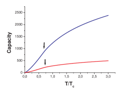
Figure 1: The channel capacity, for the case of noninteracting bosons, plotted against $T/T_{c}$. The lower curve is for the case of 100 bosons, in a 3D box with pbc. For ⁸⁷Rb atoms in such a box of volume $1\mu\mbox{m}^{3}$, thermodynamical calculations predict $T_{c}\approx 0.4\mu\mbox{K}$. The upper curve is for 500 bosons in the same trap. The thermodynamical estimations of $T_{c}$ are higher than the corresponding values that we obtain (as indicated by the arrows).

we plot ${\cal C}^{be}_{E,N}$ vs. $T/T_{c}$, for different $N$. Here $T_{c}=(2\pi\hbar^{2}/mk_{B})(N/2.612L^{3})^{2/3}$ is the critical temperature, as obtained in the thermodynamical (large $N$) limit. The capacity changes its shape from being concave to being convex with respect to temperature, at the onset of a BEC. The thermodynamical estimation of $T_{c}$ is higher than our values of $T_{c}$ for different $N$, with the gap reducing for growing $N$. Such indication of a gap has also been obtained previously (see e.g. Dalfovo ). We have checked that the predicted approximate gap in Ref. Dalfovo , is in agreement with our calculations for $N=1000$. For lower $N$ however, the prediction is no longer valid, as expected in Ref. Dalfovo . Note that the capacity increases with increasing $N$, and it has the same qualitative behavior for a 3D box without pbc, as well as for a harmonic trap.

Fermions are better carriers of information than bosons. For spin-$s$ noninteracting fermions, $n^{f}_{i}=g/(\mbox{e}^{\beta(\varepsilon_{i}-\mu^{f})}+1)$, where $g=2s+1$, and $\mu^{f}$ is the fermion chemical potential. The channel capacity (in bits) is given by (see e.g. Reichl ) ${\cal C}_{E,N}^{fd}=-g\sum_{i}\left(\frac{n^{f}_{i}}{g}\log_{2}\frac{n^{f}_{i}}{g}+(1-\frac{n^{f}_{i}}{g})\log_{2}(1-\frac{n^{f}_{i}}{g})\right)$. Again, for given $N$ and $T$, one obtains $\mu^{f}$ from average particle number conservation, which then gives the capacity.

The bosons that we have considered in this Letter are spinless. To make a fair comparison of the capacities, we consider “spinless”, i.e. polarized fermions with $g=1$. Let us start with bosons, and perform the high temperature expansion. First, we expand the fugacity $z^{b}=\mbox{e}^{\beta\mu^{b}}$ in powers of $N/S_{1}$, where $S_{k}=\sum_{i}\mbox{e}^{-k\beta\varepsilon_{i}}$, and find the coefficients from the average particle number conservation. We use this expansion to find an expansion of the $n_{i}^{b}$’s, which in turn is substituted in the formula for ${\cal C}^{be}_{E,N}$. The same calculation is done for fermions. We perform the calculation up to the third order, and find that ${\cal C}^{be}_{E,N}=(\sum_{i=1}^{3}\alpha^{b}_{i}(N/S_{1})^{i})\log_{2}\mbox{e}+\beta^{b}_{1}(N/S_{1})\log_{2}(N/S_{1})+\beta^{b}_{2}(N/S_{1})^{2}\log_{2}(N/S_{1})$, whereas ${\cal C}^{fd}_{E,N}=(\sum_{i}\alpha^{f}_{i}(N/S_{1})^{i})\log_{2}\mbox{e}+\beta^{f}_{1}(N/S_{1})\log_{2}(N/S_{1})+\beta^{f}_{2}(N/S_{1})^{2}\log_{2}(N/S_{1})$. The coefficients of first order perturbation are equal: $\alpha_{1}^{b}=\alpha_{1}^{f}=S_{1}+D_{1}$. In the next order, they differ by a sign: $\alpha_{2}^{b}=-\alpha_{2}^{f}=S_{2}/2-S_{2}D_{1}/S_{1}+D_{2}$. The third order perturbation coefficients are again equal: $\alpha_{3}^{b}=\alpha_{3}^{f}=-3S_{2}+S_{3}/3+2S_{2}^{2}/S_{1}+(2S_{2}^{2}-S_{1}S_{3})D_{1}/S_{1}^{2}-2S_{2}D_{2}/S_{1}+D_{3}$. Also, $\beta_{1}^{b}=\beta_{1}^{f}=-S_{1}$, $\beta_{2}^{b}=0$, $\beta_{2}^{f}=2S_{2}$; here $D_{k}=\sum_{i}\beta\varepsilon_{i}\mbox{e}^{-k\beta\varepsilon_{i}}$.

To find out the potentials and dimensions for which this perturbation technique is systematic, we consider uniform power law potentials, such as $V=r^{\gamma}$, in a $d$-dimensional Cartesian space of $(x_{1},\ldots,x_{d})$, with $r=\sqrt{x_{1}^{2}+\ldots+x_{d}^{2}}$. We calculate $S_{k}$ and $D_{k}$, replacing sums by integrations with density of states $\rho(\varepsilon)=\int d^{d}pd^{d}x\delta(p^{2}/2m+V-\varepsilon)$, the latter integration being over the phase space. One may then check that the technique is systematic when $1/\gamma+1/2>1/d$. This includes, e.g., the 3D and 2D harmonic potentials, for which we also performed the summations directly, and obtained the same results. Note that $0=\beta_{2}^{b}<\beta_{2}^{f}$, whereas $\alpha_{2}^{b}=S_{2}(1-\beta\left\langle\varepsilon\right\rangle_{\beta}+\beta\left\langle\varepsilon\right\rangle_{2\beta})$ (where $\left\langle\varepsilon\right\rangle_{\beta}$ stands for the average energy with Boltzmann probabilities $\mbox{e}^{-\beta\varepsilon_{i}}/S_{1}$) can be explicitly evaluated by using the density of states $\rho(\varepsilon)$. As a result, we obtain $\alpha_{2}^{b}\leq 0\leq\alpha_{2}^{f}$, implying that ${\cal C}^{be}_{E,N}<{\cal C}^{fd}_{E,N}$ for a large range of sufficiently high temperature, and for power law potentials that satisfy the same condition as systematicity. We have

Theorem. For power law potential traps (with power $\gamma$ and dimension $d$), and for sufficiently high temperature, the capacity of fermions is better than that of bosons when $1/\gamma+1/2>1/d$.

This includes, e.g., the harmonic trap in 2D and 3D, the 3D rectangular box, and the 3D spherical box. The theorem holds for quite moderate $T$, since we work up to the order $(N/S_{1})^{3}$. Numerical simulations show indeed that it holds also for low temperatures, as seen, e.g., in Fig. 2 for 100 spinless fermions and same number of spinless bosons trapped in a 3D box with pbc.

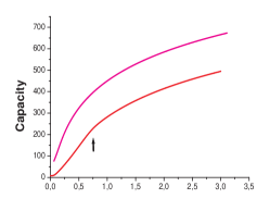
Figure 2: We compare the channel capacity for the case of 100 (noninteracting) spinless fermions (upper curve) with that of 100 bosons (lower curve). The trap is a 3D box with pbc. For the lower curve, the horizontal axis is $T/T_{c}$, while for the upper curve, it is $T/T_{f}$, where $T_{f}=(\hbar^{2}/2mk_{B})(6\pi^{2}N/gL^{3})^{2/3}$ is the Fermi temperature.

Note that we have found that the capacities for a 3D box without pbc are lower than those with pbc, both for bosons and fermions. The capacity for a harmonic trap, with the same characteristic length scale, has a higher capacity (both for bosons as well as for fermions) than that for a 3D box with pbc. More importantly, the capacities for the case of fermions do not show any signatures of criticality, as expected.

Interacting fermions. Until now, we have been dealing with the case of noninteracting bosons and fermions. Although a system of noninteracting massive bosons exhibits condensation, this is not the case for noninteracting fermions. A system of interacting fermions, however, can exhibit Cooper pairing, and, consequently, superfluid BCS transition (see e.g. Reichl ). It is therefore interesting to see whether such a “condensation” can be observed in the capacity of a channel transmitting trapped interacting fermions. We consider here a 3D box (of volume $L^{3}$) with pbc, within which $N$ fermions are trapped. The fermions behave like an ideal Fermi-Dirac gas, except when pairs of them with equal and opposite momentum, and opposite spin components have kinetic energy within an interval $\Delta\epsilon$ on either side of the Fermi surface. In that case, the pairs experience a weak attraction. The Hamiltonian can then be written as ${\cal H}=\sum_{\vec{k}}t_{\vec{k}}(a^{\dagger}_{\vec{k},\uparrow}a_{\vec{k},\uparrow}+a^{\dagger}_{\vec{k},\downarrow}a_{\vec{k},\downarrow})+\sum_{\vec{k},\vec{l}}V_{\vec{k},\vec{l}}a^{\dagger}_{\vec{k},\uparrow}a^{\dagger}_{-\vec{k},\downarrow}a_{-\vec{l},\downarrow}a_{\vec{l},\uparrow}$, where $t_{\vec{k}}=\hbar^{2}k^{2}/2m$, whereas $V_{\vec{k},\vec{l}}$ vanishes except when $|\mu-\hbar^{2}k^{2}/2m|\leq\Delta\epsilon$ and $|\mu-\hbar^{2}l^{2}/2m|\leq\Delta\epsilon$, in which case, $V_{\vec{k},\vec{l}}=-V_{0}<0$. Using mean field approximation, the average occupation number in this case turns out to be $N_{\vec{k}}=(1-(\epsilon_{\vec{k}}/E_{\vec{k}})\tanh(\beta E_{\vec{k}}/2))/2,$ where $\epsilon_{\vec{k}}=t_{\vec{k}}-\mu$, $E_{\vec{k}}=\sqrt{\epsilon_{\vec{k}}^{2}+|\Delta_{\vec{k}}|^{2}}$. Here $\Delta_{\vec{k}}=\Delta(T)$, when $|\epsilon_{\vec{k}}|\leq\Delta\epsilon$, and vanishing otherwise. This is the so-called “gap”, given by the equation, $\Delta_{\vec{l}}=V_{0}\sum_{\vec{k}}(\Delta_{\vec{k}}/E_{\vec{k}})\tanh(\beta E_{\vec{k}}/2),$ where the summation runs only for an energy interval $\Delta\epsilon$ about the Fermi surface. Note that the occupation numbers in this case are different from the case of ideal (noninteracting) fermions. Using the gap equation and the constraint $\sum_{\vec{k}}N_{\vec{k}}=N$ on the total number of fermions in the trap, we can find the channel capacity by replacing $n^{f}_{i}$ by $N_{\vec{k}}$ in ${\cal C}_{E,N}^{fd}$. As we see in Fig. 3, the channel capacity again changes its behavior qualitatively, indicating the onset of the superfluid BCS transition. In Fig. 3, we plot the channel capacity against $T/T_{f}$, where $T_{f}$ is the Fermi temperature for the case of noninteracting fermions. This is for convenience, as the thermodynamical transition temperature (for interacting fermions) has an exponentially decaying factor, which renders it inconvenient for our purposes. Also we chose $\Delta\epsilon=\frac{\hbar^{2}}{mL^{2}}$ and $V_{0}=10^{-6}\frac{\hbar^{2}}{mL^{2}}$ in the figure.

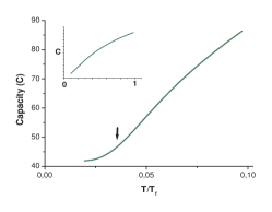
Figure 3: Channel capacity of 100 interacting fermions in a 3D box trap with pbc, against $T/T_{f}$. The capacity is initially convex, and then becomes concave, for higher $T$’s, as illustrated in the inset.

In this Letter, we have used the GCE, which has appeared due to the dual constraints of average energy and average particle number. For a fixed number of particles, and retaining the average energy constraint, we are led to CE. In the thermodynamical limit, the average occupation numbers are the same for CE and GCE. For finite $N$, exact calculations for CE are difficult. However, different approximate methods (see e.g. Nobel-kajer-por ) reveal that the average occupation numbers of CE are more uniform as compared to GCE, so that the former ensemble has larger capacity. However, the difference is marginal.

The channels that we have considered in this Letter are noiseless. A simple, but physically important, model of noise is the Gaussian noise acting similarly on each mode, resulting in an effective increase of temperature in the channel. So for a given temperature, to accomodate the average energy constraint, we must start with a lower temperature than that in the noiseless case, leading to a decrease in capacity. The lower capacity in this particular noisy case can be read off from the figures of the noiseless one after finding the temperature difference.

To conclude, we have considered the classical capacities of noiseless quantum channels carrying a finite average number of massive bosons or fermions. We have shown that the capacities are attained on the grand-canonical ensemble of statistical mechanics. Capacity of a channel carrying bosons indicates the onset of Bose-Einstein condensation, by changing its behavior from being concave to convex with respect to the temperature, at the transition point. Also the signature of the onset of Bardeen-Cooper-Schrieffer transition can be observed for weakly interacting fermions. We show analytically that for noninteracting particles, fermionic channels are better than the bosonic ones, in a wide variety of cases.

We acknowledge support from the DFG (SFB 407, SPP 1078, SPP 1116, 436POL), the Alexander von Humboldt Foundation, the Spanish MEC grant FIS-2005-04627, the ESF Program QUDEDIS, and EU IP SCALA.

References

- (1) Institució Catalana de Recerca i Estudis Avançats.
- (2) J.P. Gordon, in Proc. Int. School Phys. “Enrico Fermi, Course XXXI”, ed. P.A. Miles, pp. 156 (Academic Press, NY 1964); L.B. Levitin, in Proc. VI National Conf. Inf. Theory, Tashkent, pp. 111 (1969); A.S. Holevo, Probl. Pereda. Inf. 9, 3 1973 [Probl. Inf. Transm. 9, 110 (1973)]; H.P. Yuen in Quantum Communication, Computing, and Measurement, ed. O. Hirota et al. (Plenum, NY 1997)).
- (3) H.P. Yuen and M. Ozawa, Phys. Rev. Lett. 70, 363 (1993).
- (4) B. Schumacher, M. Westmoreland, and W.K. Wootters, Phys. Rev. Lett. 76, 3452 (1996).
- (5) P. Badzia̧g, M. Horodecki, A. Sen(De), and U. Sen, Phys. Rev. Lett. 91, 117901 (2003); M. Horodecki, J. Oppenheim, A. Sen(De), and U. Sen, ibid. 93, 170503 (2004).
- (6) C.M. Caves and P.D. Drummond, Rev. Mod. Phys. 66, 481 (1994).
- (7) A.S. Holevo, M. Sohma, and O. Hirota, Phys. Rev. A 59, 1820 (1999); A.S. Holevo and R.F. Werner, ibid. 63, 032312 (2001); V. Giovannetti, S. Lloyd, and L. Maccone, ibid. 70, 012307 (2004); V. Giovannetti et al., ibid., 032315 (2004); S. Lloyd, Phys. Rev. Lett. 90, 167902 (2003); V. Giovannetti, S. Lloyd, L. Maccone, and P.W. Shor, ibid. 91, 047901 (2003); V. Giovannetti et al., ibid. 92, 027902 (2004).
- (8) K. Bongs et al., Phys. Rev. A 63, 031602 (2001); R. Dumke et al., Phys. Rev. Lett. 89, 220402 (2002); H. Kreutzmann et al., ibid. 92, 163201 (2004).
- (9) cf. P. Hommelhoff et al., New J. Phys. 7, 3 (2005); R. Folman et al., Adv. At. Mol. Opt. Phys. 48, 263 (2002); J. Fortagh and C. Zimmermann, Science 307, 860 (2005).
- (10) K. Huang, Statistical Mechanics, (John Wiley & Sons, New York, 1987).
- (11) R.Y. Chiao et al., Phys. Rev. A 69, 063816 (2004).
- (12) F. Dalfovo, S. Giorgini, L.P. Pitaevskii, and S. Stringari, Rev. Mod. Phys. 71, 463 (1999).
- (13) L.E. Reichl, A Modern Course in Statistical Physics, (John Wiley & Sons, New York, 1998).
- (14) H.D. Politzer, Phys. Rev. A 54, 5048 (1996); M. Wilkens and C. Weiss, J. Mod. Opt. 44, 1801 (1997).