Reduction of Magnetic Noise in Atom Chips by Material Optimization

Abstract

We discuss the contribution of the material type in metal wires to the electromagnetic fluctuations in magnetic microtraps close to the surface of an atom chip. We show that significant reduction of the magnetic noise can be achieved by replacing the pure noble metal wires with their dilute alloys. The alloy composition provides an additional degree of freedom which enables a controlled reduction of both magnetic noise and resistivity if the atom chip is cooled. In addition, we provide a careful re-analysis of the magnetically induced trap loss observed by Yu-Ju Lin et al. [Phys. Rev. Lett. 92, 050404 (2004)] and find good agreement with an improved theory.
PACS numbers:
39.25.+k Atom manipulation
72.15.-v Electronic conduction in metals and alloys
07.50.-e Electrical and electronic instruments and components
03.75.-b Matter waves

1 Introduction

Much progress has been made during the last 2-3 years in the technology of atom chip fabrication and the experimental control and imaging of ultracold neutral atoms trapped near metallic and dielectric surfaces. This resulted in a significant improvement in the study of atom-surface interactions and provided reliable and reproducible information about the behavior of the atomic clouds trapped at different heights above the chip surface [1]-[7]. In magnetic traps close to the surface of the chip, atoms experience magnetic fluctuations which enhance harmful effects such as spin-flip induced trap loss, heating and decoherence. Good agreement was found between experimental measurements of these effects and their theoretical predictions presented in references [8]-[14]. A complete theoretical treatment of magnetic fluctuations close to metallic surface is based on summing the contribution of thermally occupied modes of the electromagnetic field in the presence of the metallic surface. This approach provides a manageable calculation of the magnetic fluctuations close to an infinite planar surface [8]-[11]. A different approach (the quasi-static approximation) assumes that at low transition frequencies, magnetic fluctuations are instantaneously generated by thermal electric current fluctuations in the metal [12]. This approach is not restricted to planar surfaces and is therefore suitable for calculating magnetic noise on an atom chip with complex structures. Both theoretical approaches predict the same dependence of the magnetic noise on the temperature and resistivity of the metal chip elements in the limit of a large penetration depth (low transition frequencies), although some differences occur in the dependence on the chip geometry. For a detailed review of the relevant equations, see the paper by C. Henkel in this Special Issue [15].

Atom chip surfaces have to meet stringent requirements and are conventionally made of copper and gold. Both metals are convenient in view of their ability to hold high current densities and in view of available technology (ease of evaporation, electroplating, and etching), gold being somewhat preferable due to its high resistance to corrosion. Furthermore, it appeared to be common wisdom that as the surface induced noise was a function of the ratio $T/\rho$ (quasi-static approximation) between the surface temperature and its resistivity, there is no point in cooling the surface, since $\rho$ usually scales linearly with temperature.

In this work, we discuss the possibility of minimizing the surface induced noise by a proper choice of the materials and their temperature. As an example, we discuss several materials (normal metals or alloys) and convenient temperature regimes in which one may achieve both minimal resistivity and minimal magnetic noise. Experimental data suggesting that this is indeed possible is provided by the large difference in the scattering rates observed for atom clouds trapped near different metal surfaces [4].

2 Material dependence of magnetic noise

Our analysis is based on the theory of loss and heating for magnetically trapped atoms near metallic surfaces developed in [11] and [12]. Magnetic trapping of neutral atoms is limited by transitions into untrapped Zeeman levels. The transition rate $\Gamma_{0\rightarrow f}$ from the trapped state $|0\rangle$ into an untrapped state $|f\rangle$ is proportional to the magnetic field fluctuations in the following way [11]:

$$\Gamma_{0\rightarrow f}=\sum_{i,j}\frac{\langle 0|\mu_{i}|f\rangle\langle f|\mu_{j}|0\rangle}{\hbar^{2}}S_{B}^{ij}(\omega_{f0})$$ (1)

where $\mu_{i}$ and $\mu_{j}$ ($i,j=1,2,3$) are the projections of the atomic magnetic moment on the main axes and $S^{ij}_{B}(\omega_{f0})$ is the spectral density of the magnetic noise at the transition frequency $\omega_{f0}$ (for spin-flip transitions, $\omega_{f0}$ is the Larmor frequency of the atomic spin in the center of the trap). The spectral density $S_{B}^{ij}$ is related to the two-point correlation function of the magnetic field fluctuations:

$$\langle B^{*}_{i}({\bf x},\omega)B_{j}({\bf x},\omega^{\prime})\rangle=2\pi\delta(\omega-\omega^{\prime})S_{B}^{ij}({\bf x},\omega)$$ (2)

where ${\bf x}$ is the location of the trap center. Typically, one is in the stationary limit of very low transition frequencies, where the wavelength of the radiated field is much larger than the dimensions of the system and the penetration depth of the electromagnetic field into the metal is much larger than the thickness of the metal structures. The spectral density of the magnetic noise is described in this regime by the simple product of a factor, which is material-dependent, and a geometrical tensor $Y_{ij}$ [12]:

$$S_{B}^{ij}({\bf x},\omega)=\frac{\mu_{0}^{2}k_{B}T}{4\pi^{2}\rho}Y_{ij}({\bf x})$$ (3)

where $k_{B}$ is the Boltzman constant, $\mu_{0}$ is the vacuum permeability, $T$ is the temperature of the metal, and $\rho$ its static resistivity. The geometrical tensor $Y_{ij}({\bf x})$ at the trap center is given by (note that the factor $1/2$ is erroneously missing in Eq.(A.6) of Ref. [12]):

$$Y_{ij} = {\rm tr}\{X_{ij}\}\delta_{ij}-X_{ij}$$

$$X_{ij} = \frac{1}{2}\int d^{3}{\bf x}^{\prime}\frac{({\bf x}-{\bf x}^{\prime})_{i}({\bf x}-{\bf x}^{\prime})_{j}}{({\bf x}-{\bf x}^{\prime})^{6}}$$ (4)

where the integration is done over the volume of the metal element.

The spectral density of the magnetic noise in Eq. (3) is actually independent of the transition frequency and gives rise to a scattering rate which is proportional to the ratio $T/\rho$. This result of the quasi-static approximation is valid whenever the skin depth $\delta=\sqrt{2\rho/\mu_{0}\omega_{f0}}$ is much larger than both the distance $d$ of the trap from the metal structure and the thickness $t$ of the metal structure elements.

In the opposite limit, when $\delta$ is very small, e.g. as the resistance drops upon cooling, the penetration depth is reduced according to $\delta\propto\rho^{1/2}$, and the scaling laws with $\rho$ and distance change. For example, above a metallic half-space, the quasi-static approximation ($d\ll\delta$) results in a scaling of $T/(\rho d)$ [8, 9, 12] while for $d\gg\delta$ one finds a scaling of $T\rho^{1/2}/d^{4}$ [10, 11] (see also a discussion in [15, 16]).

An expression for the magnetic noise in the intermediate range where the skin depth is comparable to the thickness or the distance, exists only for planar (possibly layered) structures in the form of interpolation formulas [8, 10] or integrals to be computed numerically (see a review in Ref. [15] and recent work in Refs. [16, 17]). For an infinitely thick metallic layer, Ref. [11] suggests an interpolation factor of $\left(1+2d^{3}/3\delta^{3}\right)^{-1}$ which should multiply the expression in Eq. (3). This factor was shown experimentally to give the right trends, but is not very accurate at intermediate distances $d\sim\delta$, where the integral expression gives a much better agreement with experiment [4]. Its important to note that in the regime of a short skin depth, $d>\delta$, the magnetic noise power is actually reduced compared to the scaling law $T/\rho$. More specifically, the large-distance scaling of $T\rho^{1/2}$ now implies a strong noise reduction upon cooling. In this work, we will mainly deal with the regime where the factor $T/\rho$ holds. However, when describing our conclusions for this regime, we will also define its validity borders and address the consequences of entering the short skin depth regime.

Taking gold at room temperature as our standard (and using similar notation as in [12]), we may write a simplified expression for $\Gamma$:

$$\Gamma\approx 57s^{-1}\frac{(T/300K)}{(\rho/\rho_{{\rm Au},300K})}\sum_{ij}\frac{\mu_{i}\mu_{j}}{\mu_{B}^{2}}(Y_{ij}\times 1\mu m)$$ (5)

where $\mu_{B}$ is the Bohr magneton, $\rho_{{\rm Au},300K}$ is the resistivity of gold at room temperature and $\mu_{i},\mu_{j}$ are matrix elements of the atomic magnetic moment between relevant states. To avoid complications of magnetic permeability and hysteresis of the chip, we consider here only nonmagnetic metals (having no long-range magnetic order). The resistivity of these metals is essentially a sum of two contributions $\rho=\rho_{0}+\rho_{\rm ph}$: a temperature independent residual resistivity $\rho_{0}$, due to scattering of charge carriers by crystal defects and impurities and a phonon contribution $\rho_{\rm ph}$, which can be described in the well known Bloch-Gruneisen approximation as [18]:

$$\rho_{\rm ph}=A\left(\frac{T}{\Theta}\right)^{5}\int_{0}^{\Theta/T}\frac{z^{5}e^{z}}{(e^{z}-1)^{2}}dz$$ (6)

where $A$ is constant and $\Theta=\hbar\omega_{\rm ph}/k_{B}$ is the Debye temperature, $\omega_{\rm ph}$ being the phonon cutoff frequency. The asymptotic temperature dependence of the phonon resistivity at very low temperatures ($T\ll\Theta$) is given by $\rho_{\rm ph}\sim T^{5}$, while it becomes linear $\rho_{\rm ph}\sim T$ at high temperatures ($T\gg\Theta$). One can then identify three regimes for the behavior of the ratio $T/\rho$ that provides upper limits for the magnetic noise, as mentioned above:

• at low temperatures the metal resistivity is dominated by the temperature independent residual resistivity $\rho_{0}$ and $T/\rho$ will decrease linearly when reducing the temperature.

• in an intermediate regime where the phonon resistivity dominates, such that $\rho\gg\rho_{0}$, but the temperature is less than the Debye temperature $\Theta$ or comparable to it, the resistivity grows nonlinearly with temperature ($\rho_{\rm ph}\sim{T^{\alpha}}$, with $\alpha>1$) and $T/\rho$ increases with reducing temperature.

• at high temperatures the resistivity becomes linear in $T$ and $T/\rho$ will be temperature independent.

For real conductors the residual resistance ratio $\varrho\equiv\rho(300{\rm K})/\rho_{0}$ (used as a quality parameter) has a wide variation due to its dependence on the purity level, as well as the thermal and mechanical treatment of the metal. Conducting elements on an atom chip are usually fabricated as a film and thereby may have significant residual resistivity relative to bulk metals. Lattice and surface disorder in metal films, which is mainly due to grain structure and gas absorption, results in the increase of $\rho_{0}$ [19].

For the comparison of the magnetic noise produced by different materials we need not specify the geometry of the conductor, which is all contained in the tensor $Y_{ij}$. In accordance with Eq. (5), we can formulate the optimization criteria as the following: the material used for the chip wires should have both the resistivity and the ratio $T/\rho$ smaller than the gold standard at $T=$300 K, in a convenient temperature interval.

3 Pure metals

Pure metals usually have high values of $\varrho$, such that for $10\,{\rm K}<T<300\,{\rm K}$, their behavior follows that of the intermediate regime defined above, where the magnetic noise increases with cooling. This situation is illustrated in Fig. 1, where the normalized magnetic noise of copper, silver, gold and niobium is presented as a function of temperature. The values are normalized to the magnetic noise level for gold at $T=$300 K. Respective resistivity behavior is shown in the inset. The data for the ideal (phonon) resistivity of the metals were extracted from [20]. We assume $\rho_{0}$ to be 1% of the room temperature resistivity (such values are realistic for high quality films of 2-3$\mu$m thickness  [21, 22]). One should note that the latter number is highly sensitive to the details of the fabrication process, including material purity, film thickness, granular structure and surface specularity. As can be seen from Fig. 1, the magnetic noise from the studied noble metals is not reduced by cooling but rather exhibits a pronounced peak in the temperature range 20-50 K.

As mentioned above in the discussion following Eq. (3) and (4), we need to define the validity borders of the $T/\rho$ approximation. As an example, we consider a trap with a spin-flip transition frequency $\omega_{f0}\approx 2\pi\times 0.79$MHz ($B_{0}$=0.57G) near a copper-made conductor, as in the experiment described in Ref. [5]. The skin depth for copper with $\varrho$=100 is $\delta=74\mu$m at room temperature ($\rho=1.7\mu\Omega\cdot$cm), $\delta=25.3\mu$m at liquid nitrogen temperature ($\rho=0.2\mu\Omega\cdot$cm) and $\delta=7.4\mu$m at liquid helium temperature ($\rho=0.017\mu\Omega\cdot$cm). Following the explanation given above, our analysis of pure metals at low temperatures will be restricted to trap distances from the surface of less than $\delta$, namely, less than 7$\mu$m at liquid helium temperatures. Some corrections will be needed for distances close to 7$\mu$m and a separate treatment will be needed for longer distances. For higher temperatures, or for alloys with higher resistivity as in the next section, or for lower transition frequencies such as transitions between motional levels in magnetic traps (heating), the following analysis will be valid for distances of at least several tens of microns.

Figure 1: Temperature dependence of the normalized magnetic noise calculated using Eq. (5) for wires made of copper (circles), silver (triangles) gold (crosses) and niobium (squares). The noise is normalized to the value for gold at $T=$300 K. Inset: temperature dependence of the resistivity (extracted from [20]).

In order to broaden the search we have performed the magnetic noise calculation for 14 metals having no magnetic ordering: Al, W, Au, Ir, Cu, Mo, Nb, Pt, Rh, Ag, Ta, Ti, Zn, Zr. The resistivity data for the metals were extracted from [20]. It is convenient to plot the normalized noise vs. the normalized resistivity at constant temperature. In accordance with Eq. (5), this plot gives a straight line with unit negative slope if plotted in a double logarithmic scale. The results of the analysis for the temperature of $T=$77 and 20 K are displayed in Fig. 2. Both the noise and resistivity data are normalized to those of gold at $T=$300 K (thus, points appearing in the area restricted by the solid lines correspond to values better than those of gold at room temperature). We may observe that at least three metals (molybdenum, zinc and platinum) at liquid nitrogen temperature and two metals (zirconium and titanium) at $T=$20 K have better characteristics than those of gold at $T=$300 K. For example, Ti-made wires cooled down to 20 K will have a factor three reduction in the noise and four-fold reduction in the resistivity relative to gold at room temperature.

Figure 2: Dependence of the $T/\rho$ ratio (normalized to its value for gold at 300 K) on the normalized resistivity at $T=$77 and 20 K for various metals. The dashed lines correspond to the theoretical dependencies of the noise on the resistivity for the given temperatures (see Eq. (3)). Metals having qualities better than those of gold at 300 K, are indicated in bold letters.

Finally, let us note that in this analysis we are considering only the magnetic noise reduction due to the $T/\rho$ ratio appearing in Eq. (3). The geometrical factor $Y_{ij}$ may also contribute to noise reduction because it depends on wire thickness. As the resistivity drops with cooling, wire thickness may be reduced while maintaining the same current. However, this may give rise to problems such as enhanced relative surface roughness, which may in turn enhance harmful effects such as fragmentation. In addition, thickness reduction is limited as thinner films have an increased resistivity.

4 Alloys

More promising materials for a cooled atom chip could be found among nonmagnetic dilute metal alloys, whose residual resistivity is usually higher than in pure metals. In alloys, such residual resistivity may be set to a desired value by adjusting the material composition. The resistivity of a dilute binary alloy is given by

$$\rho(x,T)=\rho_{0}(x)+\rho_{\rm ph}(T)+\Delta(x,T),$$ (7)

where the residual resistivity $\rho_{0}$ is proportional to the concentration $x$ of the solute metal and $\rho_{\rm ph}$ is the phonon resistivity of the solvent metal, which is not changed by the addition of the solute metal, according to the well known Matthiessen’s rule. The last term in Eq. (7), $\Delta(x,T)$, is a correction to the Mathiessen’s rule, which was intensively investigated in the literature (see, for example, [23]). This deviation represents a change in the temperature dependence of the resistivity at low temperatures and moderate solute concentrations and its measurement is important for the study of scattering mechanisms in metals and alloys (for more details see Refs. [23]-[26]). However, its value relative to the total resistivity is small. Figure 3 shows the measured values of resistivity for Ag-Au alloys at different concentrations and temperatures. The inset shows that the deviation $\Delta$ from the Matthiessen’s rule is less than 10% for Au concentrations between 0.1% and 10%. At concentrations as high as 2% or more it is negligible. In the following analysis we will therefore neglect the correction term $\Delta$ and assume that the Matthiessen’s rule is a good approximation for the calculation of the magnetic noise.

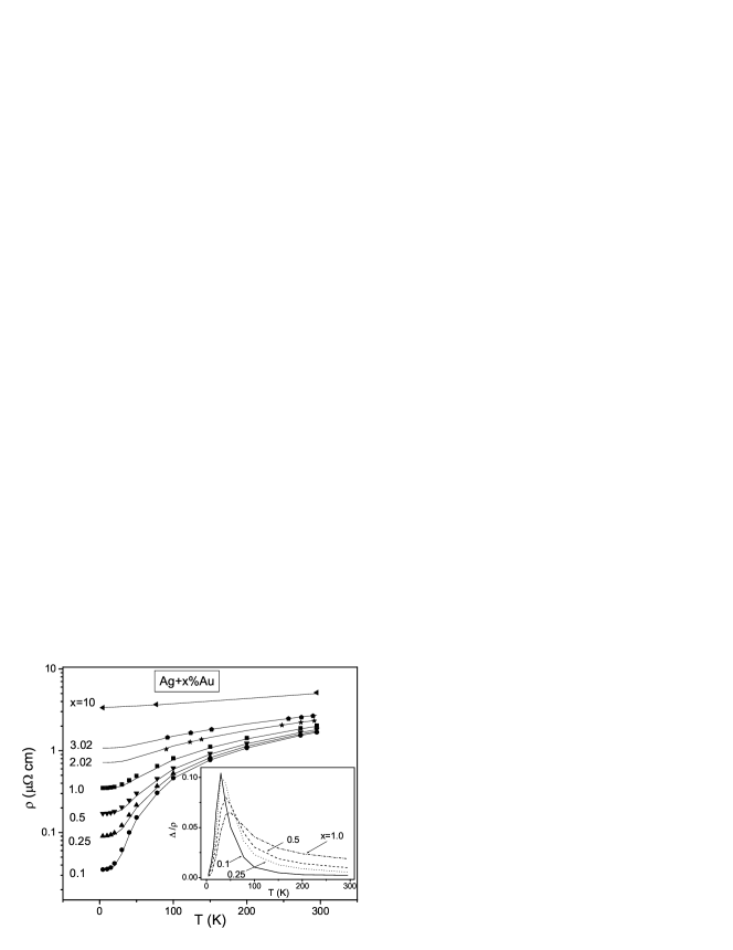
Figure 3: Measured resistivity of Ag-Au alloys with different concentrations as a function of temperature [24, 28, 29]. Solid lines are the predicted values according to the Matthiessen’s rule. Inset: temperature dependence of the ratio of the deviation $\Delta(x,T)$ from the Matthiessen’s rule to the total Ag-Au alloy resistivity for small Au concentrations.

If the solute concentration is not very high (up to $x=$10-15%, where ordering processes may start changing the behavior) the residual resistivity of the alloy $\rho_{0}(x)$ increases linearly with increasing component ratio [23, 24, 27]. This concentration dependent residual resistivity provides an additional degree of freedom which can be controlled in order to obtain the desired magnetic noise and resistivity of the chip material. The concentration of the solute should not be too large. In accordance with our optimization criteria, the alloy is effective as a chip wire material if its total resistivity does not exceed gold resistivity at room temperature. In Fig. 4 the temperature behavior of the normalized ratio $T/\rho$ is shown for a set of dilute Ag-Au alloys as well as for pure silver. The temperature dependencies $\rho(T$) for the alloys were calculated using Eq. (7). The phonon resistivity data of silver ($\rho_{{\rm ph,\,Ag}}(T)$) were extracted from [20], and the experimental values of the residual resistivity ($\rho_{0}(x)$) for different gold concentrations $x$ were extracted from references [24] and [30].

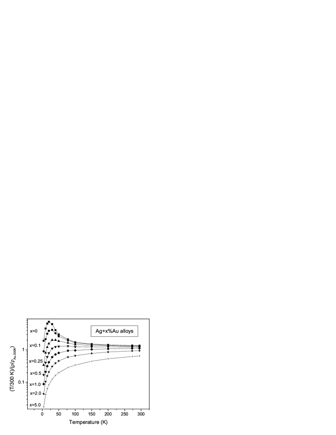
Figure 4: Temperature dependence of the ratio $T/\rho$ (normalized to its value for gold at 300 K) for silver and its alloys with gold: pure silver (squares), and with 0.1% gold (circles), 0.25% (triangles), 0.5% (inverted triangles), 1% (diamonds), 2% (stars), and 5% (crosses). The $\rho(T)$ dependence for alloys was calculated using the residual resistivity data given by [24, 30]. Note the difference compared to Fig. 1.

From Fig. 4 one may conclude that the low temperature maximum in $T/\rho$, which is intrinsic for pure metals (Fig. 1), disappears with increasing $x$. This behavior is general for most of the dilute alloys. In particular, it is valid for the alloys we analyze in the following. In Fig. 5 we plot the normalized noise vs. normalized resistivity characteristics of the alloys Ag-Au, Cu-Au and Cu-Ge. As an example, the cooling of wires made of the alloy Ag+5%Au down to $T=$77 K can reduce the noise by a factor of 5 relative to the level of pure silver at room temperature, and by a factor 3 relative to gold. The latter factor is almost the same as that achieved, for example, for Pt in Fig. 2, but due to the unique alloy phenomena described above (Fig. 4), a pronounced difference will appear between Pt and Ag+5%Au as the temperature is lowered further.

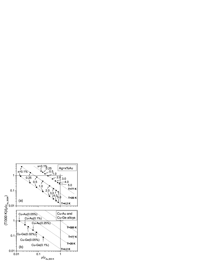
Figure 5: Normalized noise ($T/\rho$) and resistivity characteristics for dilute alloys. The values for $T/\rho$ and resistivity are normalized to those of gold at 300 K. (a) Ag-Au alloys, (b) Cu-Au and Cu-Ge alloys. For (b) the solute concentration is given in brackets. The residual resistivity data for alloys are extracted from  [24] and  [30].

According to Eq. (3), the product of the magnetic noise and the resistivity is linearly proportional to the temperature and independent of the material (as indicated by the sloped straight lines in Fig. 5). A cooling procedure would reduce the magnetic noise relative to the magnetic noise of gold at room temperature by a factor $(T/300K)\cdot(\rho_{{\rm Au},300K}/\rho_{Alloy}(T))$. It is possible to choose the alloy concentration such that $\rho_{\rm Alloy}(T)=\rho_{{\rm Au},300K}$, so that the resistivity will be kept at the gold standard but the magnetic noise will be reduced by a factor of $T/$300K. Hence, the noise of an alloy-made conductor could be reduced relative to the gold standard maximally by 4 times when cooling to liquid nitrogen temperature ($T=$77 K) and by 70 times by cooling to liquid helium temperature ($T=$4.2 K). This ratio of noise reduction is reached on the boundary of the optimization area. In particular, for the alloys Ag-Au, Cu-Au and Cu-Ge, the solute concentrations on this boundary equal 6%, 4.5% and 0.52% respectively (for $T=$4.2 K). The values were obtained from the $\rho_{0}(x)$ dependencies presented in [24, 29].

Thus, the main conclusion of this paper is that a significant simultaneous reduction of magnetic noise and resistivity is possible with both pure metals and alloys at 77K, and may be reduced even further by making use of alloys and further cooling. We note that a further advantage of wires made of alloys relative to pure metals, may perhaps be found in the fact that their resistivity is less sensitive to temperature fluctuations, since it is mainly due to the residual resistivity. This fact may contribute to current stability under temperature variations in space (along the wire) or time.

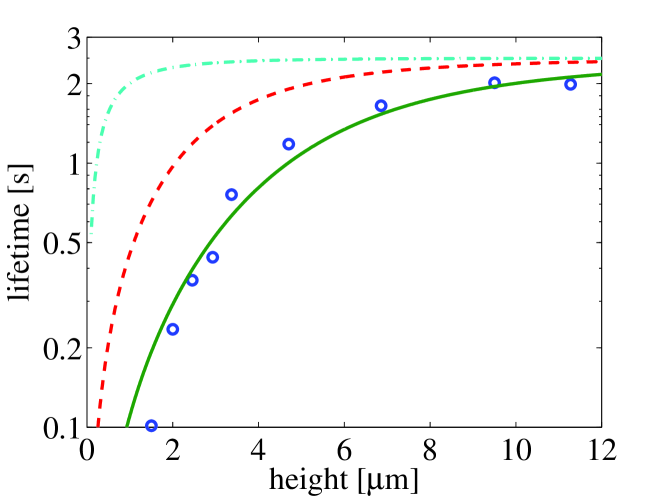
Figure 6: Comparison of trapping lifetimes of ⁸⁷Rb atoms above a copper wire on an atom chip [5] with a theoretical calculation (solid line). Predicted lifetimes are also shown for a similar wire made of an alloy of Ag with 6% Au content, cooled down to $T=$77K (dashed) and 4.2K (dash-dotted). In both cases the resistivity was taken equal to gold resistivity at $T$=300 K, $\rho_{\rm Au}=2.21\mu\Omega\cdot$cm (same penetration depth). According to Fig.  5a, the needed gold concentrations are estimated by $x=5.4$% and $x=6$%, respectively. Note that our calculation differs from the one made in [5] (see Appendix A). Van der Waals forces are not taken into account. Let us also mention that the maximum noise reduction factor of 70 noted in the text, is not visible, due to the effect of the technical noise and/or background gas collisions limiting the lifetime in this experiment to a maximum of $\tau_{\rm tech}=2.5\,s$ [31].

In order to illustrate the effect of noise reduction on the lifetime of trapped atoms we present the predicted lifetime of ⁸⁷Rb close to a metal wire similar to that used in Ref. [5]. Fig. 6 shows the experimental results together with a theoretical curve simulating the experiment with the copper wire at $T=$400 K ($\rho_{\rm Cu}=2.64\mu\Omega\cdot$cm). Details of the calculation are given in Appendix A (note that our calculation is different from that made in [5]). No fitting parameters were used, except for assuming a distance independent scattering rate of 0.4 s^-1[5, 31]. The predicted lifetimes for a similar wire made of the alloy Ag+6%Au, and cooled down to $T=$77K or 4.2K, are also presented. They show that lifetimes can be increased by more than an order of magnitude. When cooling down to 4.2K, the atomic lifetime is close to the limit set by (distance independent) background scattering even when the atoms are held 1$\mu m$ from the wire.

As suggested by Fig. 1, the magnetic noise will not be reduced by cooling the copper wires, as long as it obeys the $T/\rho$ law. However, as the temperature becomes smaller, one approaches the regime where the penetration depth $\delta$ gets shorter than characteristic scales like the trap height $d$, and the $T/\rho$ law must be amended. As mentioned before, in the simple case of an infinitely thick metal layer, the noise power can be multiplied by the interpolation factor $(1+2d^{3}/3\delta^{3})^{-1}$ to get the scaling for short skin depth [11]. At large distances, the $T/(\rho d)$ law is thus replaced by the asymptotic law $\frac{3}{2}(2/\mu_{0}\omega_{f0})^{3/2}T\sqrt{\rho}/d^{4}$ with a more favorable scaling with temperature. In Figure 7 we compare the noise (relative to the standard of gold at room temperature) for a Ag-Au alloy and for a copper wire at 4.2 K, as a function of distance. It is seen that the noise from a cooled copper wire drops below the noise from a wire made of an alloy only at $d>45\mu$m. This value is expected to be even bigger if a wire thickness $t<\delta$ would be taken into account. We recall that the interpolation factor mentioned above actually overestimates the magnetic noise power, as illustrated in Ref.[11] and in Ref. [4] by comparing to numerical calculation and experimental data, respectively. The maximal observed discrepancy is about a factor of 3 at $d=\delta$. On the other hand, one can expect an increase of the pure metal $\delta$ at cold temperatures, due to the fact that typical pure metal wires have larger residual resistivities than the numbers used in our calculation. For example, Ref. [5] calculated $\delta=103\,\mu{\rm m}$ while our calculation uses $\varrho=100$ which leads to $\delta=92\,\mu{\rm m}$. In summary, it follows that as far as magnetic noise is concerned, cooled wires made of alloys are preferable over cooled wires made of pure metals over a large range of distances from the atom chip.

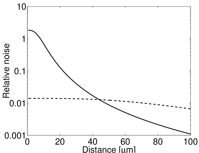
Figure 7: Magnetic noise relative to the room temperature gold standard for an Ag-Au alloy (dashed line) at a temperature of 4.2 K and for a pure copper wire at 4.2 K (solid line) as a function of distance from the chip. The noise was calculated based on the interpolation formula of Ref. [11] (see text). The penetration depths used for copper and the Ag-Au alloy are $\delta=7.4\mu$m and $\delta=84\mu$m, respectively.

Finally, we consider in Appendix B the feasibility of cooling current carrying wires to low temperatures. We analyze the expected heating due to the ohmic resistance and find that for considerable current densities, the temperature rise in the wires does not significantly alter the results presented in this paper.

5 Conclusions

We have analyzed the dependence of magnetic fluctuations near the surface of conducting elements on an atom chip, on the material type and the temperature. We have shown that at low temperatures a significant reduction of the noise can be achieved by making the conducting wires from dilute alloys of noble metals.

This improvement is due to the large value of the temperature independent residual resistivity of the alloys compared to pure noble metals, which is controllable by smoothly changing the solute component concentration. At least three important advantages of cooling wires made of alloys could be underlined: (i) reduction of the magnetic noise, thereby decreasing loss rate, heating and decoherence; (ii) possible reduction of the resistivity of the wires, and (iii) enhancement of temperature stability. With the data presented in this work, it is possible to identify alloys that reach a minimum noise level that is set by that of the expected technical noise.

Finally, we note that for optimal noise reduction, a complete optimization is required for every specific situation. Such an optimization should take into account not only the $T/\rho$ ratio analyzed in this work, but also the geometrical factor, which includes important parameters such as wire thickness, and trap height (see the discussion in Ref. [17] for flat wires). We note that the geometrical parameters also define the validity borders of the $T/\rho$ approximation, and corrections have to be applied when the penetration depth becomes comparable to wire thickness or trap height.

Appendix A Comparison between predicted and measured magnetic noise for thin rectangular wires

For calculating the magnetic noise close to a rectangular metal wire of width $w$ and thickness $t$ we have calculated the tensor $Y_{ij}$ of Eq. (4) for a slab extending from $y^{\prime}=-\infty$ to $y^{\prime}=\infty$, from $x^{\prime}=-w/2$ to $x^{\prime}=w/2$ and from $z^{\prime}=-t$ to $z^{\prime}=0$. The results of the integration for nonzero elements $Y_{ij}$ are:

$$Y_{11} = \frac{3}{8}{\rm tr}\{Y_{ij}\}+\frac{\pi}{16}\left[\left[\frac{v}{u}\frac{1}{\sqrt{u^{2}+v^{2}}}\right]_{u=-w/2-x}^{w/2-x}\right]_{v=-z-t}^{-z}$$ (8)

$$Y_{22} = \frac{3}{8}{\rm tr}\{Y_{ij}\}=-\frac{3\pi}{16}\left[\left[\frac{\sqrt{u^{2}+v^{2}}}{uv}\right]_{u=-w/2-x}^{w/2-x}\right]_{v=-z-t}^{-z}$$ (9)

$$Y_{33} = \frac{3}{8}{\rm tr}\{Y_{ij}\}+\frac{\pi}{16}\left[\left[\frac{u}{v}\frac{1}{\sqrt{u^{2}+v^{2}}}\right]_{u=-w/2-x}^{w/2-x}\right]_{v=-z-t}^{-z}$$ (10)

$$Y_{31} = \frac{\pi}{16}\left[\left[\frac{1}{\sqrt{u^{2}+v^{2}}}\right]_{u=-w/2-x}^{w/2-x}\right]_{v=-z-t}^{-z}$$ (11)

where we have used the definition

$$\left[\left[f(u,v)\right]_{u=a}^{b}\right]_{v=c}^{d}\equiv f(a,c)-f(a,d)-f(b,c)+f(b,d).$$ (12)

In Ref. [5] the lifetime of trapped atoms was measured above the center of a rectangular copper wire of thickness $t=2.15\mu m$ and width $w=10\mu m$. The temperature of the wire was estimated as 400 K ($\rho_{\rm Cu}=2.64\mu\Omega\cdot$cm). The measurements were performed with ⁸⁷Rb atoms trapped in the hyperfine state $|F,m\rangle=|2,2\rangle$. The loss process was assumed to be due to the cascade of transitions $|2,2\rangle\rightarrow|2,1\rangle\rightarrow|2,0\rangle$. By use of Eq. (1) and Eq. (3) we obtain for this kind of transitions

$$\Gamma_{|F,m\rangle\rightarrow|F,m-1\rangle}=\frac{\mu_{0}^{2}\mu_{B}^{2}g_{F}^{2}k_{B}T}{4\pi^{2}\rho}\sum_{j}Y_{jj}\left|\langle F,m|F_{j}|F,m-1\rangle\right|^{2}$$ (13)

where we have substituted $\mu_{j}=\mu_{B}g_{F}F_{j}$. The contribution of off-diagonal terms of $Y_{ij}$ vanishes, given the symmetric position above the center of the wire.

In Ref. [5], the total lifetime of the trapped states due to magnetic noise was approximated to be $\tau_{mag}\approx\tau_{1}+\tau_{2}$, where $\tau_{2}$ and $\tau_{1}$, which are the lifetimes of the respective levels $|2,2\rangle$ and $|2,1\rangle$, are equal to the inverse of the transition rates $\gamma_{21}=\Gamma_{|2,2\rangle\rightarrow|2,1\rangle}$ and $\gamma_{10}=\Gamma_{|2,1\rangle\rightarrow|2,0\rangle}$. A complete approach should take into account that the transition frequency between the magnetic levels is in the order of MHz, while the temperature of the surface is several orders of magnitude larger. This means that the atoms have an equal probability for transitions from $|2,2\rangle$ into $|2,1\rangle$ and vice versa. We assume that atoms that decayed into the untrapped level $|2,0\rangle$ escape immediately from the trap region. The rate equations are then

$$\frac{d}{dt}P_{|2,2\rangle} = -\gamma_{21}(P_{|2,2\rangle}-P_{|2,1\rangle})$$ (14)

$$\frac{d}{dt}P_{|2,1\rangle} = \gamma_{21}(P_{|2,2\rangle}-P_{|2,1\rangle})-\gamma_{10}P_{|2,1\rangle}$$ (15)

$$\frac{d}{dt}P_{|2,0\rangle} = \gamma_{10}P_{|2,1\rangle}$$ (16)

For our calculation, we make use of $|\langle 2,2|F_{j}|2,1\rangle|^{2}=1$ and $|\langle 2,1|F_{j}|2,0\rangle|^{2}=3/2$ for $j=x,z$, where we assume the direction of the magnetic field to be along the wire axis ($y$ direction). We thus have $\gamma_{10}/\gamma_{21}=3/2$, and the solution to the rate equations yields

$$P_{mag}=P_{|2,2\rangle}+P_{|2,1\rangle}=\frac{1}{5}\left[6e^{-\gamma_{21}t/2}-e^{-3\gamma_{21}t}\right]$$ (17)

This gives an effective ($1/{\rm e}$) lifetime of $\tau=2.364\gamma_{21}^{-1}$.

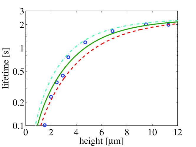
Figure 8: The trapping lifetimes of ⁸⁷Rb atoms above a wire on an atom chip for the data presented in Ref. [5]. The plot presents a comparison between the two calculation methods presented in the text and the calculation of Ref. [5] (dash-dotted line). The dashed line represents the taking into account of transitions in one direction only while the solid line represents the complete approach.

In Fig. 8 we compare this calculation (solid line) to the simpler model described above where $\tau_{\rm mag}=\tau_{1}+\tau_{2}$ (dashed line), while using the same geometrical factors. For completeness, we also present the calculation of ref. [5] (dash-dotted line), who have used an interpolated formula for the geometrical factor. The experimental trap lifetime is restricted by technical noise and/or background gas collisions to a maximum of $\tau_{\rm tech}=2.5\,s$ [31]. Hence the total trap lifetime is equal to $\tau_{\rm trap}=(\tau_{\rm mag}^{-1}+\tau_{\rm tech}^{-1})^{-1}$. The geometrical factors $Y_{ij}$ were calculated using Eqs. (9)-(11). We see that the complete approach (solid line) gives a better agreement with experiment than the calculation based on the simplified model (dashed line). Based on this comparison, we make use of the complete approach, and present in Fig. 6 the expected trap lifetime for the alloy Ag-Au for different cooling temperatures.

Hopefully, one would be able to construct a more complete theory that is compatible with the full theory presented in ref. [11], while still enabling a practical calculation of finite structures [15]. We then expect that at low heights above the surface (smaller than the penetration depth in the metal), the parallel components $Y_{11}$ and $Y_{22}$ will decrease by a factor of 1/3, giving rise to an increase of the calculated lifetime by a factor of 5/3. On the other hand, the measurements of ref. [5] were performed with a thermal atomic cloud of temperature 1$\,\mu$K. One then expects that the cloud expands in the $x,z$ directions to a radius of $\sim 0.5\,\mu$m, so that the loss rate is significantly increased for the fraction of atoms that are closer to the metal surface. The deformation of the trapping potential due to atom-surface interactions of the van der Waals type (not included in Fig. 6) may also contribute to an increased loss rate. These effects may perhaps explain the noted difference between all the calculated curves and the experimental results at low heights above the surface.

Appendix B Feasibility of cooling current carrying wires

In Ref. [32] it was shown that the heating of a metal wire on an atom chip is characterized by two time scales: a fast time scale related to heat transfer through the contact and/or insulating layer from the metal into the substrate followed by slow heating due to heat transfer in the substrate. Heat transfer through the contact and/or insulating layer depends on the heat conductivity $k$ of these layers. For a single contact layer of effective thickness $d_{c}$ and heat conductivity $\lambda_{c}$ the number $k$ is given by $k=\lambda_{c}/d_{c}$. For a wire of width $w$, thickness $h$ and resistivity $\rho(T)$ the equation of heat transfer is

$$hC_{W}\frac{\partial}{\partial t}\Delta T=h\rho(T)j^{2}-k\Delta T,$$ (18)

where $C_{W}$ is the heat capacity of the metal, $h\rho j^{2}$ is the rate of generation of heat per unit wire area and $\Delta T=T-T_{0}$ is the temperature rise above the substrate temperature $T_{0}$. To get a rough estimate of $\Delta T$ after the heating we assume here that $\rho(T)$ is constant within $\Delta T$ (for instance, as presented in Fig. 5a, the resistivity of our example alloy Ag+5%Au hardly changes in the range of 4-77K). We then obtain a steady state value of $\Delta T$:

$$\Delta T=h\rho j^{2}/k\,.$$ (19)

The process of slow heating was modeled in Ref. [32] in a two dimensional model with an analytic and numeric solution. It was found that the slow temperature rise is given by

$$\Delta T_{s}=\frac{hw\rho j^{2}}{2\pi\lambda}\ln\left(\frac{4\pi^{2}\lambda t}{Cw^{2}}\right),$$ (20)

where $C$ and $\lambda$ are the heat capacity and conductivity of the substrate, respectively.

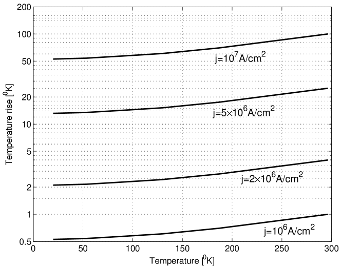
Figure 9: Temperature rise in a current carrying wire as a function of the initial system temperature, and for different current densities. The wire geometry was taken to be as in Ref. [32]. The temperature rise includes the fast rise and a slow rise for 30s.

Typical values of $\Delta T$ as a function of the initial temperature are given in Fig. LABEL:fig7 for a few values of current density $j$. The temperature rise contains the fast heating and slow heating after $30$s. The calculation was done for the geometry of Ref. [32], namely $w=5\mu$m, $h=1.4\mu$m and $\rho=\rho_{\rm Au,300\,K}$. Since the dependence of the heating on the current density $j$ is quadratic, it follows that if the temperature of a wire holding a current density of $10^{7}$ A/cm² rises by 50 K, then a wire with current density of 10⁶A/cm² heats only by 0.5 K.

We may conclude that the reduction of magnetic noise by cooling will always be limited by wire heating if the current density in the wire is large. The heating will still be negligible for current densities of the order of $10^{6}$A/cm² or less. One should note that improved geometries, such as wires buried in the wafer (thus transferring heat to the wafer through 3 facets), will further improve the allowed current densities.

References

- [1] J. Fortagh, H. Ott, S. Kraft, A. Gunther, and C. Zimmermann. Phys. Rev. A, 66, 041604(R) (2002); H. Ott, J. Fortagh, G. Schlotterbeck, A. Grossmann, and C. Zimmermann, Phys. Rev. Lett. 87, 230401 (2001).
- [2] A. E. Leanhardt, Y. Shin, A. P. Chikkatur, D. Kielpinski, W. Ketterle, and D. E. Pritchard. Phys. Rev. Lett. 90, 100404 (2003).
- [3] M. P. A. Jones, C. J. Vale, D. Sahagun, B. V. Hall, and E. A. Hinds. Phys. Rev. Lett. 91, 080401 (2003).
- [4] D. M. Harber, J. M. McGuirck, J. M. Obrecht, and E. A. Cornell. J. Low. Temp. Phys. 133, 229 (2003). cond-mat/0307546.
- [5] Y. Lin, I. Teper, C. Chin, and V. Vuletić, Phys. Rev. Lett. 92, 050404 (2004).
- [6] P. Krüger Ph.D. Thesis (2004); P. Krüger et al., cond-mat/0504686 (2005).
- [7] P. Treutlein, P. Hommelhoff, T. Steinmetz, T. W. Hönsch, and J. Reichel, Phys. Rev. Lett. 92, 203005 (2004).
- [8] T. Varpula and T. Poutanen. J. Appl. Phys. 55, 4015 (1984)
- [9] J. Nenonen, J. Montonen, and T. Katila. Review of Scientific Instruments, 67, 2397 (1996)
- [10] J. A. Sidles, J. L. Garbini, W. M. Dougherty, and S. H. Chao, Proc. IEEE 91, 799 (2003); arXiv:quant-ph/0004106
- [11] C. Henkel, S. Pötting, and M. Wilkens, Appl. Phys. B 69, 379 (1999).
- [12] C. Henkel, S. Pötting, Appl. Phys. B 72, 73 (2001).
- [13] R. Folman, P. Krüger, J. Schmiedmayer, J. Denschlag, and C. Henkel Adv. At. Mol. Opt. Phys. 48, 263 (2002).
- [14] C. Henkel, P. Krüger, R. Folman, and J. Schmiedmayer Appl. Phys. B 76, 173 (2003).
- [15] C. Henkel, paper in this special issue.
- [16] S. Scheel, P. K. Rekdal, P. L. Knight, and E. A. Hinds, arXiv:quant-ph/0501149 (2005).
- [17] B. Zhang, C. Henkel, E. Haller, S. Wildermuth, S. Hofferberth, Peter Krüger, and J. Schmiedmayer, article in this Special Issue.
- [18] Ziman J. M. Electrons and Phonons, Oxford: Oxford University Press, 1960.
- [19] P. Wissmann The electrical resistivity of pured and gas covered metal films. In Springer Tracts in Modern Physics V. 77, Springer-Verlag 1975.
- [20] M. P. Malkov, I. B. Danilov, A. G. Zeldovich, and A. B. Fradkov. Handbook on Physical and Technical Basis of Cryogenics, Energiya, Moskwa, 1973.
- [21] A. von Bassewitz, E. N. Mitchell, Phys. Rev. 182, 712 (1969).
- [22] J. R. Sambles, K. C. Elsom and G. Sharp-Dent, J. Phys. F (Metal Phys.) 11, 1075 (1981).
- [23] J. Bass, Advan. Phys. 21, 431 (1972).
- [24] J. S. Dugdale, Z. S. Basinski Phys. Rev. 157, 552 (1967).
- [25] F. Nakamura, K. Ogasavara, and J. Takamura, J. Phys. F, 6, L11 (1976).
- [26] I. A. Campbell, A. D. Caplin, C. Rizzuto, Phys. Rev. Lett. 26, 239 (1971).
- [27] H. A. Fairbank Phys. Rev. 66, 274 (1944).
- [28] J. O. Linde Ann. Phys. 14, 353 (1932).
- [29] T. H. Davis, J. A. Rayne, Phys. Rev. B 6, 2931 (1972).
- [30] Thesis by J. O. Linde (unpublished) given by F. J. Blatt in Solid State Physics edited by F. Seitz and D. Turnbull (Academic, New York, 1957), p.318.
- [31] Yu-Ju Lin, Private communications.
- [32] S. Groth, P. Kruger, S. Wildermuth S, et al., Appl. Phys. Lett. 85, 2980 (2004).