Noiseless method for checking the Peres separability criterion by local operations and classical communication

Abstract

We present a method for checking Peres separability criterion in an arbitrary bipartite quantum state $\rho_{\mbox{\tiny\rm AB}}$ within local operations and classical communication scenario. The method does not require the prior state reconstruction and the structural physical approximation. The main task for the two observers, Alice and Bob, is to estimate some specific functions. After getting these functions, they can determine the minimal eigenvalue of $\rho^{T_{\mbox{\tiny\rm B}}}_{\mbox{\tiny\rm AB}}$, which serves as an entanglement indicator in lower dimensions.

I I. introduction

Quantum entanglement epr ; sch ; bel has been an important physical resource for quantum information processings nch , for example, quantum teleportation, quantum key distribution, and quantum dense code. Before we can make use of the entanglement, we need know that it really exists in the system. The first and most widely used criterion is the Peres separability criterion, i.e. the positive partial transpose (PPT) criterion per ; hhh . If a quantum state $\rho_{\mbox{\tiny\rm AB}}$ has matrix elements $\rho_{ij}^{mn}=\langle ij|\rho_{\mbox{\tiny\rm AB}}|mn\rangle$ then the partial transpose $\rho_{\mbox{\tiny\rm AB}}^{T_{\mbox{\tiny\rm B}}}$ is defined as

$$(\rho_{ij}^{mn})^{T_{\mbox{\tiny\rm B}}}=\rho_{in}^{mj}.$$ (1)

The criterion is known if $\rho_{\mbox{\tiny\rm AB}}$ is separable, then it must have a PPT. Thus any state for which $\rho_{\mbox{\tiny\rm AB}}^{T_{\mbox{\tiny\rm B}}}$ is not positive semidefinite is necessarily entangled. When we deal with an unknown quantum state, we can resort to quantum state tomography vor which provides the full knowledge about the density matrix. However, there are more efficient ways that compute the entangled properties directly via some functions of density matrix $\rho_{\mbox{\tiny\rm AB}}$. A. Ekert and P. Horodecki et al. have done a series of works eke ; pho ; pha ; phl ; car on entanglement detection and measurement in an unknown mixed state without the prior state reconstruction. These methods rely on two techniques: the first is a modified interferometer network eke inserted a controlled-$U$ operation (for the analysis c.f. sjo ; fil ); the second is the structural physical approximation (SPA) pho , which achieve a non-physical map approximately by mixing in an appropriate proportion the noise operation $D(\rho)=I/d$. The SPA could tackle the problem of some non-physical operation, but its practical implementation is difficult. Recently, H. Carteret hac constructed some networks that can determine the eigenvalues of the partially transposed density matrix $\rho_{\mbox{\tiny\rm AB}}^{T_{\mbox{\tiny\rm B}}}$, without resorting to the SPA. This method is efficient and feasible for the physical implementation.

In quantum communication, it is important to detect the entanglement within local operations and classical communication (LOCC) scenario, in which the two observers, Alice and Bob, are far apart from each other and share a composite system. It has been proven that entanglement is a precondition for secure quantum key distribution mcu . Based on the PPT criterion, C.M. Alves et al. presented a scheme to test the entanglement with the aid of the LOCC implementation of the SPA car . But the physical implementation of the SPA is of more difficult in the LOCC version.

In this paper, we present an LOCC method to check the Peres separability criterion, an extension of H. Carteret’s method hac . Our method is feasible for the physical implementation in the LOCC scenario, because the SPA is not necessary. The main task for Alice and Bob is to estimate some specific functions of density matrix $\rho_{\mbox{\tiny\rm AB}}$ via two local networks. After getting these functions, they can determine the spectrum of the matrix $\rho_{\mbox{\tiny\rm AB}}^{T_{\mbox{\tiny\rm B}}}$ in which the minimal eigenvalue is an entanglement witness.

This paper is organized as follows. In Sec. II, we present the LOCC method for checking Peres separability criterion without SPA. Then we discuss our method in Sec. III. Finally, in Sec. IV, we give some conclusions.

II II. checking the PPT criterion by LOCC

To see how the LOCC method works, we first recapitulate the global method. In Ref. hac , H. Carteret constructed some global networks for estimating the eigenvalues of the partial transposed matrix $\rho_{\mbox{\tiny\rm AB}}^{T_{\mbox{\tiny\rm B}}}$ without resorting to the SPA. In general form, the network can be described by using Fig.1.

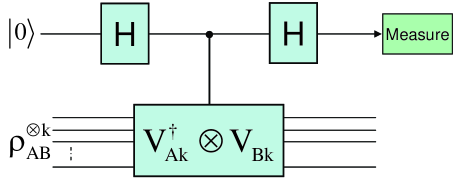
Figure 1: General form of Carteret’s network, which can estimate the eigenvalues of the partial transposed matrix $\rho_{\mbox{\tiny\rm AB}}^{T_{\mbox{\tiny\rm B}}}$.

The method is partially inspired by the modified interferometer network eke ; sjo , in which a controlled-$U$ operation is inserted between two Hadamard gates. When one measures the control qubit in the computational basis, the modification of interference pattern is given by eke

$$\mbox{Tr}(U\rho)=ve^{i\alpha},$$ (2)

where $v$ is the visibility and $\alpha$ is the phase shift. H. Carteret chooses the controlled-$U$ to be two controlled cyclic permutations hac , which is equivalent to the controlled-$V_{Ak}^{\dagger}\otimes V_{Bk}$ as shown in Fig.1. The unitary shift operator $V_{k}$ is defined as eke

$$V_{k}|\phi_{1}\rangle|\phi_{2}\rangle\cdots|\phi_{k}\rangle=|\phi_{k}\rangle|\phi_{1}\rangle\cdots|\phi_{k-1}\rangle,$$ (3)

and $V_{Ak}^{\dagger}$ and $V_{Bk}$ act on the subsystems $A$ and the subsystems $B$, respectively. By measuring the control qubit, one can get the function $\mbox{Tr}[(V_{Ak}^{\dagger}\otimes V_{Bk})\rho_{\mbox{\tiny\rm AB}}^{\otimes k}]$, which can be expanded into

$$\mbox{Tr}[(V_{Ak}^{\dagger}\otimes V_{Bk})\rho_{\mbox{\tiny\rm AB}}^{\otimes k}]$$ (4)

$$= \mbox{Tr}\left[\sum\rho_{i_{1}j_{1}}^{m_{1}n_{1}}\rho_{i_{2}j_{2}}^{m_{2}n_{2}}\cdots\rho_{i_{k}j_{k}}^{m_{k}n_{k}}|i_{1}j_{k}\rangle\langle m_{k}n_{1}|\otimes|i_{2}j_{1}\rangle\langle m_{1}n_{2}|\otimes\cdots\otimes|i_{k}j_{k-1}\rangle\langle m_{k-1}n_{k}|\right]$$

$$= \sum\rho_{i_{1}j_{1}}^{i_{2}j_{k}}\rho_{i_{2}j_{2}}^{i_{3}j_{1}}\cdots\rho_{i_{k}j_{k}}^{i_{1}j_{k-1}}.$$

Combining with Eq. (1), one can get the following relation

$$\mbox{Tr}[(V_{Ak}^{\dagger}\otimes V_{Bk})\rho_{\mbox{\tiny\rm AB}}^{\otimes k}]=\mbox{Tr}[(\rho_{\mbox{\tiny\rm AB}}^{T_{\mbox{\tiny\rm B}}})^{k}]=\sum_{i=1}^{d}\lambda_{i}^{k},$$ (5)

in which $d$ denotes the dimension of $\rho_{\mbox{\tiny\rm AB}}$ and $\lambda_{i}$ is the eigenvalue of $\rho_{\mbox{\tiny\rm AB}}^{T_{\mbox{\tiny\rm B}}}$. Thus, by measuring $(d-1)$ functions, one can determine the spectrum of $\rho_{\mbox{\tiny\rm AB}}^{T_{\mbox{\tiny\rm B}}}$.

In this paper, we present an LOCC method to check the Peres separability criterion without resorting the SPA. It is assumed that Alice and Bob share a number of the unknown quantum states $\rho_{\mbox{\tiny\rm AB}}$. The main task of the two observers is to estimate the function $\mbox{Tr}[(\rho_{\mbox{\tiny\rm AB}}^{T_{\mbox{\tiny\rm B}}})^{k}]$ within the LOCC scenario. A normal LOCC network for the task is shown in Fig.2.

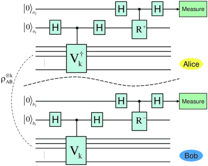
Figure 2: A normal network for remote estimation of the eigenvalues of the partial transposed matrix $\rho_{\mbox{\tiny\rm AB}}^{T_{\mbox{\tiny\rm B}}}$. By estimating the probabilities $P_{a_{2}b_{2}}(ij)$ that the two ancillary qubits $a_{2}b_{2}$ is found in state $|ij\rangle$, Alice and Bob can get the function $\mbox{Tr}[(\rho_{\mbox{\tiny\rm AB}}^{T_{\mbox{\tiny\rm B}}})^{k}]$.

The network is composed of four modified interferometer circuits. The first part for Alice is a modified interferometer circuit which is attached to a controlled-$V_{Ak}^{\dagger}$ gate. The ancillary qubit $a_{1}$ is the control qubit and the subsystems $\rho_{\mbox{\tiny\rm A}}^{\otimes k}$ is the target. The second part following the first is another interferometer circuit which is attached to a controlled-$R^{+}$ gate. In this part, $a_{2}$ is the control qubit and $a_{1}$ is the target qubit. The circuit for Bob is similar to that for Alice except for some controlled quantum gates. In the following analysis, we will show that Alice and Bob can get the requisite function as long as they estimate the probabilities $P_{a_{2}b_{2}}(ij)$ that in the measurement the two ancillary qubits $a_{2}$ and $b_{2}$ are found in the state $|ij\rangle$ where $i,j=0,1$.

We consider the first part of Alice and Bob’s circuits. The input state is

$$\rho_{in}(k)=\rho_{\mbox{\tiny\rm AB}}^{\otimes k}\otimes\rho_{a_{1}}\otimes\rho_{b_{1}},$$ (6)

where $\rho_{a_{1}}=|0\rangle\langle 0|$ and $\rho_{b_{1}}=|0\rangle\langle 0|$ are the initial states of the ancillary qubits. The Hadamard gate and the controlled-$U$ gate in their networks can be written as

$$H=\frac{1}{\sqrt{2}}\left(\begin{array}[]{cc}1&1\\ 1&-1\\ \end{array}\right)$$ (14)

$$U_{C-U}=\left(\begin{array}[]{cc}1&0\\ 0&0\\ \end{array}\right)\otimes I+\left(\begin{array}[]{cc}0&0\\ 0&1\\ \end{array}\right)\otimes U$$

in the computational basis. After the two modified interferometer circuits, the input state transforms into the following state

$$\rho^{\prime}_{out}(k)=U_{h}U_{v}U_{h}\rho_{in}(k)U_{h}^{{\dagger}}U_{v}^{{\dagger}}U_{h}^{{\dagger}},$$ (15)

where $U_{h}=H_{a_{1}}\otimes H_{b_{1}}\otimes I_{\mbox{\tiny\rm AB}}^{\otimes k}$ and $U_{v}=U_{C-V_{A2k}^{\dagger}}\otimes U_{C-V_{B2k}}$. In the state $\rho^{\prime}_{out}(k)$, what we concern is the state evolution of the two ancillary qubits $a_{1}$ and $b_{1}$. After some deduction, we can obtain that the state of the two ancillary qubits transforms into

$$\rho^{\prime}_{a_{1}b_{1}}(k) = \mbox{Tr}_{AB}[\rho^{\prime}_{out}(k)]$$ (20)

$$= \frac{1}{4}\left(\begin{array}[]{cccc}1+\mu_{1}^{(k)}+\mu_{3}^{(k)}&\mu_{5}^{(k)}&\mu_{5}^{(k)}&-\mu_{4}^{(k)}\\ -\mu_{5}^{(k)}&1-\mu_{2}^{(k)}-\mu_{3}^{(k)}&\mu_{4}^{(k)}&-\mu_{5}^{(k)}\\ -\mu_{5}^{(k)}&\mu_{4}^{(k)}&1+\mu_{2}^{(k)}-\mu_{3}^{(k)}&-\mu_{5}^{(k)}\\ -\mu_{4}^{(k)}&\mu_{5}^{(k)}&\mu_{5}^{(k)}&1-\mu_{1}^{(k)}+\mu_{3}^{(k)}\\ \end{array}\right),$$

where

$$\mu_{1}^{(k)} = \mbox{Tr}[(V_{Ak}\otimes I_{Bk})\rho_{\mbox{\tiny\rm AB}}^{\otimes k}]+\mbox{Tr}[(I_{Ak}\otimes V_{Bk})\rho_{\mbox{\tiny\rm AB}}^{\otimes k}],$$

$$\mu_{2}^{(k)} = \mbox{Tr}[(V_{Ak}\otimes I_{Bk})\rho_{\mbox{\tiny\rm AB}}^{\otimes k}]-\mbox{Tr}[(I_{Ak}\otimes V_{Bk})\rho_{\mbox{\tiny\rm AB}}^{\otimes k}],$$

$$\mu_{3}^{(k)} = \frac{1}{2}\mbox{Tr}[(V_{Ak}\otimes V_{Bk})\rho_{\mbox{\tiny\rm AB}}^{\otimes k}]+\frac{1}{4}\mbox{Tr}[(V_{Ak}^{{\dagger}}\otimes V_{Bk})\rho_{\mbox{\tiny\rm AB}}^{\otimes k}]+\frac{1}{4}\mbox{Tr}[(V_{Ak}\otimes V_{Bk}^{{\dagger}})\rho_{\mbox{\tiny\rm AB}}^{\otimes k}],$$

$$\mu_{4}^{(k)} = \frac{1}{2}\mbox{Tr}[(V_{Ak}\otimes V_{Bk})\rho_{\mbox{\tiny\rm AB}}^{\otimes k}]-\frac{1}{4}\mbox{Tr}[(V_{Ak}^{{\dagger}}\otimes V_{Bk})\rho_{\mbox{\tiny\rm AB}}^{\otimes k}]-\frac{1}{4}\mbox{Tr}[(V_{Ak}\otimes V_{Bk}^{{\dagger}})\rho_{\mbox{\tiny\rm AB}}^{\otimes k}],$$

$$\mu_{5}^{(k)} = \frac{1}{4}\mbox{Tr}[(V_{Ak}^{{\dagger}}\otimes V_{Bk})\rho_{\mbox{\tiny\rm AB}}^{\otimes k}]-\frac{1}{4}\mbox{Tr}[(V_{Ak}\otimes V_{Bk}^{{\dagger}})\rho_{\mbox{\tiny\rm AB}}^{\otimes k}].$$ (21)

Before considering the second part of the LOCC network, we need to analyze Eq. (10) in detail. The shift operator $V_{k}$ has the property phl

$$\mbox{Tr}(V_{k}\rho_{1}\otimes\rho_{2}\cdots\otimes\rho_{k})=\mbox{Tr}(\rho_{1}\rho_{2}\cdots\rho_{k}).$$ (22)

Based on the property, we can obtain $\mbox{Tr}[(V_{Ak}\otimes I_{Bk})\rho_{\mbox{\tiny\rm AB}}^{\otimes k}]=\mbox{Tr}(\rho_{\mbox{\tiny\rm A}}^{k})$, $\mbox{Tr}[(I_{Ak}\otimes V_{Bk})\rho_{\mbox{\tiny\rm AB}}^{\otimes k}]=\mbox{Tr}(\rho_{\mbox{\tiny\rm B}}^{k})$ and $\mbox{Tr}[(V_{Ak}\otimes V_{Bk})\rho_{\mbox{\tiny\rm AB}}^{\otimes k}]=\mbox{Tr}(\rho_{\mbox{\tiny\rm AB}}^{k})$. In Eq. (5), we have $\mbox{Tr}[(V_{Ak}^{\dagger}\otimes V_{Bk})\rho_{\mbox{\tiny\rm AB}}^{\otimes k}]=\mbox{Tr}[(\rho_{\mbox{\tiny\rm AB}}^{T_{\mbox{\tiny\rm B}}})^{k}]$. The partial transposed matrix $\rho_{\mbox{\tiny\rm AB}}^{T_{\mbox{\tiny\rm B}}}$ is an Hermitian matrix, therefore its eigenvalues are real. Combining with the relation $\mbox{Tr}(U^{\dagger}\rho)=[\mbox{Tr}(U\rho)]^{\ast}$, we can get

$$\mbox{Tr}[(V_{Ak}\otimes V_{Bk}^{{\dagger}})\rho_{\mbox{\tiny\rm AB}}^{\otimes k}]=\mbox{Tr}[(V_{Ak}^{{\dagger}}\otimes V_{Bk})\rho_{\mbox{\tiny\rm AB}}^{\otimes k}].$$ (23)

Thus, in Eq. (10), the parameter $\mu_{5}^{(k)}$ equals zero. Now the state of the ancillary qubits $a_{1}$ and $b_{1}$ can be written in the following form

$$\rho^{\prime}_{a_{1}b_{1}}(k) = \frac{1}{4}\left(\begin{array}[]{cccc}1+\mu_{1}^{(k)}+\mu_{3}^{(k)}&0&0&-\mu_{4}^{(k)}\\ 0&1-\mu_{2}^{(k)}-\mu_{3}^{(k)}&\mu_{4}^{(k)}&0\\ 0&\mu_{4}^{(k)}&1+\mu_{2}^{(k)}-\mu_{3}^{(k)}&0\\ -\mu_{4}^{(k)}&0&0&1-\mu_{1}^{(k)}+\mu_{3}^{(k)}\\ \end{array}\right),$$ (28)

where

$$\mu_{1}^{(k)} = \mbox{Tr}(\rho_{\mbox{\tiny\rm A}}^{k})+\mbox{Tr}(\rho_{\mbox{\tiny\rm B}}^{k}),$$

$$\mu_{2}^{(k)} = \mbox{Tr}(\rho_{\mbox{\tiny\rm A}}^{k})-\mbox{Tr}(\rho_{\mbox{\tiny\rm B}}^{k}),$$

$$\mu_{3}^{(k)} = \frac{1}{2}\mbox{Tr}(\rho_{\mbox{\tiny\rm AB}}^{k})+\frac{1}{2}\mbox{Tr}[(\rho_{\mbox{\tiny\rm AB}}^{T_{\mbox{\tiny\rm B}}})^{k}],$$

$$\mu_{4}^{(k)} = \frac{1}{2}\mbox{Tr}(\rho_{\mbox{\tiny\rm AB}}^{k})-\frac{1}{2}\mbox{Tr}[(\rho_{\mbox{\tiny\rm AB}}^{T_{\mbox{\tiny\rm B}}})^{k}].$$ (29)

In the second part of Alice and Bob’s circuits, the input state is $\rho^{\prime}_{a_{1}b_{1}}(k)\otimes\rho_{a_{2}b_{2}}$, which is subjected to two controlled operations $U_{C-R^{+}}$ and $U_{C-R^{-}}$, where

$$R^{+}=\frac{1}{\sqrt{2}}(\sigma_{z}+\sigma_{y})=\frac{1}{\sqrt{2}}\left(\begin{array}[]{cc}1&-i\\ i&-1\\ \end{array}\right),$$ (32)

$$R^{-}=\frac{1}{\sqrt{2}}(\sigma_{z}-\sigma_{y})=\frac{1}{\sqrt{2}}\left(\begin{array}[]{cc}1&i\\ -i&-1\\ \end{array}\right).$$ (35)

The initial state of the two control qubits $a_{2}$ and $b_{2}$ is $\rho_{a_{2}b_{2}}=|00\rangle\langle 00|$. Beyond the second part, the output state will be

$$\rho_{out}(k)=U_{h}U_{r}U_{h}[\rho^{\prime}_{a_{1}b_{1}}(k)\otimes\rho_{a_{2}b_{2}}]U_{h}^{{\dagger}}U_{r}^{{\dagger}}U_{h}^{{\dagger}},$$ (36)

where $U_{r}=U_{C-R^{+}}\otimes U_{C-R^{-}}$. What we care about is the evolution of the state $\rho_{a_{2}b_{2}}$. After some deduction, we can obtain

$$\rho^{out}_{a_{2}b_{2}}(k) = \frac{1}{4}\left(\begin{array}[]{cccc}1+\mu_{1}^{(k)}+\eta^{(k)}&0&0&0\\ 0&1-\mu_{2}^{(k)}-\eta^{(k)}&0&0\\ 0&0&1+\mu_{2}^{(k)}-\eta^{(k)}&0\\ 0&0&0&1-\mu_{1}^{(k)}+\eta^{(k)}\\ \end{array}\right),$$ (41)

where $\eta^{(k)}=\mu_{3}^{(k)}-\mu_{4}^{(k)}=\mbox{Tr}[(\rho_{\mbox{\tiny\rm AB}}^{T_{\mbox{\tiny\rm B}}})^{k}]$. With the aid of a classical communication, Alice and Bob can estimate their probabilities $P_{a_{2}b_{2}}(ij)$ that in the measurement the two qubits are found in the state $|ij\rangle_{a_{2}b_{2}}$, here $i,j=0,1$. According to these probabilities, they can get the function $\mbox{Tr}[(\rho_{\mbox{\tiny\rm AB}}^{T_{\mbox{\tiny\rm B}}})^{k}]$, because

$$\eta^{(k)}=\mbox{Tr}[(\rho_{\mbox{\tiny\rm AB}}^{T_{\mbox{\tiny\rm B}}})^{k}]=P_{a_{2}b_{2}}(00)-P_{a_{2}b_{2}}(01)-P_{a_{2}b_{2}}(10)+P_{a_{2}b_{2}}(11).$$ (42)

Therefore, for any $d_{\mbox{\tiny\rm A}}\otimes d_{\mbox{\tiny\rm B}}$ dimensional quantum state $\rho_{\mbox{\tiny\rm AB}}$, Alice and Bob can determine the eigenvalues of the partial transposed matrix $\rho_{\mbox{\tiny\rm AB}}^{T_{\mbox{\tiny\rm B}}}$ by estimating the function $\mbox{Tr}[(\rho_{\mbox{\tiny\rm AB}}^{T_{\mbox{\tiny\rm B}}})^{k}]$ for $k=2,3,\cdots,d_{\mbox{\tiny\rm A}}d_{\mbox{\tiny\rm B}}$. If the minimal eigenvalue $\lambda_{min}$ is negative, the quantum state $\rho_{\mbox{\tiny\rm AB}}$ must be entangled. This concludes our description of checking Peres separability criterion within the LOCC scenario.

III III. discussions

Among the functions $\mbox{Tr}[(\rho_{\mbox{\tiny\rm AB}}^{T_{\mbox{\tiny\rm B}}})^{k}]$, $\mbox{Tr}[(\rho_{\mbox{\tiny\rm AB}}^{T_{\mbox{\tiny\rm B}}})^{2}]$ is a particular one. This is because $V_{2}$ is the only Hermitian operator, compared with the other shift operators $V_{k}$. According to Eq. (5), we have hac

$$\mbox{Tr}[(\rho_{\mbox{\tiny\rm AB}}^{T_{\mbox{\tiny\rm B}}})^{2}]=\mbox{Tr}[\rho_{\mbox{\tiny\rm AB}}^{2}].$$ (43)

Inserting Eq. (18) in Eq. (13), we can see that the quantum state $\rho^{\prime}_{a_{1}b_{1}}(2)$ has the same form as that of $\rho^{out}_{a_{2}b_{2}}(2)$. So, Alice and Bob can obtain the eigenvalues of $\rho_{\mbox{\tiny\rm AB}}^{T_{\mbox{\tiny\rm B}}}$ by estimating the probabilities $P_{a_{1}b_{1}}(ij)$. This means the second part of the network is needless for estimating $\mbox{Tr}[(\rho_{\mbox{\tiny\rm AB}}^{T_{\mbox{\tiny\rm B}}})^{2}]$. In this case, the LOCC network shown in Fig.2 is the same as the network presented by C.M. Alves et al car .

In Eq. (12), based on the Hermitian property of $\rho_{\mbox{\tiny\rm AB}}^{T_{\mbox{\tiny\rm B}}}$, we have proved $\mbox{Tr}[(V_{Ak}^{{\dagger}}\otimes V_{Bk})\rho_{\mbox{\tiny\rm AB}}^{\otimes k}]=\mbox{Tr}[(V_{Ak}\otimes V_{Bk}^{{\dagger}})\rho_{\mbox{\tiny\rm AB}}^{\otimes k}]$. The former function is $\mbox{Tr}[(\rho_{\mbox{\tiny\rm AB}}^{T_{\mbox{\tiny\rm B}}})^{k}]$. Now we reanalyze the latter function,

$$\mbox{Tr}[(V_{Ak}\otimes V_{Bk}^{\dagger})\rho_{\mbox{\tiny\rm AB}}^{\otimes k}]$$ (44)

$$= \mbox{Tr}\left[\sum\rho_{i_{1}j_{1}}^{m_{1}n_{1}}\rho_{i_{2}j_{2}}^{m_{2}n_{2}}\cdots\rho_{i_{k}j_{k}}^{m_{k}n_{k}}|i_{k}j_{1}\rangle\langle m_{1}n_{k}|\otimes|i_{1}j_{2}\rangle\langle m_{2}n_{1}|\otimes\cdots\otimes|i_{k-1}j_{k}\rangle\langle m_{k}n_{k-1}|\right]$$

$$= \sum\rho_{i_{1}j_{1}}^{i_{k}j_{2}}\rho_{i_{2}j_{2}}^{i_{1}j_{3}}\cdots\rho_{i_{k}j_{k}}^{i_{k-1}j_{1}}.$$

Having considered the definition of partial transposition, we can get

$$\mbox{Tr}[(V_{Ak}\otimes V_{Bk}^{\dagger})\rho_{\mbox{\tiny\rm AB}}^{\otimes k}]=\mbox{Tr}[(\rho_{\mbox{\tiny\rm AB}}^{T_{\mbox{\tiny\rm A}}})^{k}].$$ (45)

Therefore, in Fig.2, if Alice chooses the controlled-$V_{Ak}$ gate and Bob chooses the controlled-$V_{Bk}^{\dagger}$ gate, they can estimate the eigenvalues of $\rho_{\mbox{\tiny\rm AB}}^{T_{\mbox{\tiny\rm A}}}$. In fact, $\rho_{\mbox{\tiny\rm AB}}^{T_{\mbox{\tiny\rm B}}}$ and $\rho_{\mbox{\tiny\rm AB}}^{T_{\mbox{\tiny\rm A}}}$ have the same eigenvalues. Because, based on Eq. (12), we have $\mbox{Tr}[(\rho_{\mbox{\tiny\rm AB}}^{T_{\mbox{\tiny\rm B}}})^{k}]=\mbox{Tr}[(\rho_{\mbox{\tiny\rm AB}}^{T_{\mbox{\tiny\rm A}}})^{k}]$.

Our LOCC method is more efficient compared with the LOCC quantum state tomography. For an unknown two-qubit state, the LOCC quantum tomography needs to estimate 15 parameters of $\mbox{Tr}[(\sigma_{Ai}\otimes\sigma_{Bj})\rho_{\mbox{\tiny\rm AB}}]$ where $\sigma_{i},\sigma_{j}=I_{2},\sigma_{x},\sigma_{y},\sigma_{z}$. However, our LOCC method needs to estimate only 3 parameters, i.e. $\mbox{Tr}[(\rho_{\mbox{\tiny\rm AB}}^{T_{\mbox{\tiny\rm B}}})^{2}]$, $\mbox{Tr}[(\rho_{\mbox{\tiny\rm AB}}^{T_{\mbox{\tiny\rm B}}})^{3}]$ and $\mbox{Tr}[(\rho_{\mbox{\tiny\rm AB}}^{T_{\mbox{\tiny\rm B}}})^{4}]$. In addition, compared with the LOCC method presented by C.M. Alves et al. car , our method is more feasible in the sense of physics since Alice and Bob need not perform the SPA within the LOCC scenario. Furthermore, the quantum network shown in Fig.2 is within the reach of quantum technology currently developed.

For higher-dimensional bipartite systems, the Peres separability criterion is only the necessary condition for entanglement detection. There is a special type of quantum state— bound entangled state hla ; ppp , which has the property of PPT. A.C. Doherty et al. presented the notation of the PPT symmetric extensions drl ; doh , which is a necessary and sufficient condition for detecting bipartite entanglement. How to efficiently check the PPT symmetric extension without the prior state reconstruction is a considerable problem.

IV IV. conclusions

In this paper, we present a method for checking the Peres separability criterion without resorting to the prior state reconstruction and the SPA, which is an LOCC extension of H. Carteret’s method hac . The LOCC method is more efficient than the LOCC quantum state tomography. In addition, the method is more feasible in the physical implementation than the LOCC method presented by C.M. Alves et al car .

V acknowledgements

This work was supported by the National Natural Science Foundation of China (Grant Nos. 60325416 and 60328407) and the Special Foundation for State Major Basic Research Program of China (Grant No. G2001CB309500).

References

• (1) A. Einstein, B. Podolsky, and N. Rosen, Phys. Rev. 47, 777 (1935).
• (2) E. SchrΓΆdinger, Naturwissenschaften 23, 807 (1935); 23, 823 (1935); 23, 844 (1935).
• (3) J.S. Bell, Physics (Long Island City, New York) 1, 195 (1964).
• (4) M.A. Nielsen and I.L. Chuang, Quantum Computation and Quantum Information (Cambridge University Press, Cambridge, England, 2000).
• (5) A. Peres, Phys. Rev. Lett. 77, 1413 (1996)
• (6) M. Horodecki, P. Horodecki, and R. Horodecki, Phys. Lett. A 223, 1 (1996).
• (7) K. Vogel, H. Risken, Phys. Rev. A 40, R2847 (1989).
• (8) A.K. Ekert, C.M. Alves, D.K.L. Oi, M. Horodecki, P. Horodecki, and L.C. Kwek, Phys. Rev. Lett. 88, 217901 (2002).
• (9) P. Horodecki, Phys. Rev. A 68, 052101 (2003).
• (10) P. Horodecki and A. Ekert, Phys. Rev. Lett. 89, 127902 (2002).
• (11) P. Horodecki, Phys. Rev. Lett. 90, 167901 (2003).
• (12) C.M. Alves, P. Horodecki, D.K.L. Oi, L.C. Kwek, and A.K. Ekert, Phys. Rev. A 68, 032306 (2003).
• (13) E. SjΓΆqvist, A.K. Pati, A. Ekert, J.S. Anandan, M. Ericsson, D.K.L. Oi, and V. Vedral, Phys. Rev. Lett. 85, 2845 (2000).
• (14) R. Filip, Phys. Rev. A 65 062320 (2002).
• (15) H.A. Carteret, Phys. Rev. Lett. 94, 040502, (2005).
• (16) M. curty, M. Lewentsein and N. LΓΌtkenhaus, Phys. Rev. Lett. 92, 217903 (2004).
• (17) P. Horodecki, Phys. Lett. A 232, 333 (1997).
• (18) M. Horodecki, P. Horodecki, and R. Horodecki, Phys. Rev. Lett. 80, 5239 (2000).
• (19) A.C. Doherty, P.A. Parrilo, and F.M. Spedalieri, Phys. Rev. Lett. 88, 187904 (2002).
• (20) A.C. Doherty, P.A. Parrilo, and F.M. Spedalieri, Phys. Rev. A 69, 022308 (2004).