Stochastic simulations of conditional states of partially observed systems, quantum and classical

Abstract

In a partially observed quantum or classical system the information that we cannot access results in our description of the system becoming mixed, even if we have perfect initial knowledge. That is, if the system is quantum the conditional state will be given by a state matrix $\rho_{r}(t)$, and if classical, the conditional state will be given by a probability distribution $P_{r}(x,t)$, where $r$ is the result of the measurement. Thus to determine the evolution of this conditional state, under continuous-in-time monitoring, requires a numerically expensive calculation. In this paper we demonstrate a numerical technique based on linear measurement theory that allows us to determine the conditional state using only pure states. That is, our technique reduces the problem size by a factor of $N$, the number of basis states for the system. Furthermore we show that our method can be applied to joint classical and quantum systems such as arise in modeling realistic (finite bandwidth, noisy) measurement.

I Introduction

To obtain information about a system, a measurement has to be made. Based on the results of this measurement we assign to the system our state of knowledge. For a classical system this state takes the form of a probability distribution $P(x^{\prime},t)$, while for a quantum system we have a state matrix $\rho(t)$. In this paper we are concerned with efficient simulation techniques for partly observed systems; that is, systems for which the observer cannot obtain enough information to assign the system a pure state, $P(x^{\prime},t)=\delta[x^{\prime}-x(t)]$ or $\rho(t)=|{\psi(t)}\rangle\langle{\psi(t)}|$.

The chief motivation for wishing to know the conditional state of a system is for the purpose of feedback control Jac93 ; Bel87 ; WisMil94 ; DohJac99 . That is because for cost functions that are additive in time, the optimal basis for controlling the system is the observer’s state of knowledge about the system. Even if such a control strategy is too difficult to implement in practice, it plays the important role of bounding the performance of any strategy, which helps in seeking the best practical strategy.

It is well known that the quantum state of an open quantum system, given continuous-in-time measurements of the bath, follows a stochastic trajectory through time BelSta92 . In the quantum optics community this is referred to as a quantum trajectory Car93a ; GarParZol92 ; MolCasDal93 ; WisMil93a ; GoeGra93 ; GoeGra94 ; Wis96 ; GamWis01 ; WisDio01 ; GarZol00 . The form of this trajectory can be either jump-like in nature or diffusive depending on how we choose to measure the system; that is, the arrangement of the measuring apparatus. In this paper we review quantum trajectory theory for partially observed systems by presenting a simple model: A three level atom that emits into two separate environments, only one of which is accessible to our detectors. Such partially observed systems cannot be described by a stochastic Schrödinger  equation (SSE) Car93a ; GarParZol92 ; MolCasDal93 , but rather requires a more general form of a quantum trajectory that has been called a stochastic master equation (SME) WisMil93a . This is an instance of the fact that the most general form of quantum measurement theory requires the full Kraus representation of operations Kra83 ; BraKha92 , rather than just measurement operators BraKha92 .

It is also well known that if we have a classical system and we make measurements on it with a measurement apparatus that has associated with it a Gaussian noise, then the evolution of this classical state in the continuous-in-time limit obeys a Kushner-Stratonovich equation (KSE) Mcg74 . To review these dynamics for partially observed classical systems we present the KSE for a system that experiences an ‘internal’ unobservable white noise process. That is, the evolution in the absence of the measurements is given by a Fokker-plank equation Gar85 . This is the classical analogue to the quantum master equation.

The new work in this paper is a simple numerical technique that allows us to reduce the numerical resources required to calculate the continuous-in-time trajectories. This method relies on the implementation of linear or ‘ostensible’ Wis96 measurement theory, classical Mcg74 and quantum GoeGra93 ; GoeGra94 ; Wis96 ; GamWis01 . For the classical case our method reduces the problem from solving the KSE for the probability distribution to simulating the ensemble average of two coupled stochastic differential equations (SDE). For the quantum case our method reduces the problem from solving a conditional SME to simulating the ensemble average of a SSE plus a c-number SDE. Thus in both the classical and the quantum case, our method reduces the size of the problem by a factor of $N,$ the number of basis states required to represent the system.

Recently Brun and Goan Brun have used a similar idea to investigate a partially observed quantum system. However, since they did not use measurement theory with ostensible probabilities, their claim that they can generate a typical trajectory conditioned on some partial record ${\bf R}$ is not valid. This is demonstrated in detail in A. (In their method, the record ${\bf R}$ can only be generated randomly, and can be found only by doing the ensemble average over the fictitious noise, but that is not the issue of concern here.)

Finally, we combine these theories to consider the following case: a quantum system is monitored continuously in time by a classical system but we only have access to the results of non-ideal measurements performed on the classical system. Note that such joint systems have recently been studied by Warszawski et al WarWisMab01 ; WarWis03a ; WarGamWis04 and Oxtoby et al Neil . Warszawski et al considered continuous-in-time monitoring of a quantum optical system with realistic photodections while Oxtoby et al considered continuous-in-time monitoring of a quantum solid-state system with a quantum point contact. We show that our ostensible numerical technique can be applied to these types of systems, greatly simplifying the simulations.

The format of this paper is as follows. In Secs. II and III we review quantum and classical measurement theory respectively. This is essential as it allows us to define both the notations and the physical insight that will be used throughout this paper. In Secs. IV, V, and VI we investigate the above mentioned quantum, classical and joint systems respectively, and present our ostensible numerical technique for each specific case. Finally in Sec. VII we conclude with a discussion.

II Quantum Measurement theory (QMT)

II.1 General theory

In quantum mechanics the most general way we can represent the state of the system is via a state matrix $\rho(t)$. This is a positive semi-definite operator that acts in the system Hilbert space ${\cal H}_{\rm s}$. In this paper we take the view that this represents our state of knowledge of the system. Taking this view allows us to simply interpret the “collapse of the wavefunction”, upon measurement, as an update in the observer’s knowledge of the system CavFucSch02 ; Fuc02 . If we now assume that we have a measurement apparatus that allows us to measure observable $R$ of the system, then the conditional state $\rho_{r}(t^{\prime})$ of the system given result $r$ is determined by Kra83

$$\rho_{r}(t^{\prime})=\frac{\hat{\cal O}_{r}(t^{\prime},t)\rho(t)}{P(r,t^{\prime})},$$ (1)

where $P(r,t^{\prime})$ is the probability of getting result $r$ at time $t^{\prime}=t+T$, where $T$ is the measurement duration time. Here $\hat{\cal O}_{r}(t^{\prime},t)$ is known as the operation of the measurement and is a completely positive superoperator and for efficient measurements can be defined by

$$\hat{\cal O}_{r}(t^{\prime},t)\rho(t)=\hat{\cal J}[\hat{M}_{r}(T)]\rho(t)=\hat{M}_{r}(T)\rho(t)\hat{M}_{r}^{\dagger}(T),$$ (2)

where $\hat{M}_{r}(T)$ is called a measurement operator. The probability of getting result $r$ is given by

$$P(r,t^{\prime})={\rm Tr}[\hat{\cal O}_{r}(t^{\prime},t)\rho(t)]={\rm Tr}[\hat{F}_{r}(T)\rho(t)],$$ (3)

where the set $\{\hat{F}_{r}(T)=\hat{M}_{r}^{\dagger}(T)\hat{M}_{r}(T)\}$ is the positive operator measure (POM) for observable $R$. By completeness, the sum of all the POM elements satisfies

$$\sum_{r}\hat{F}_{r}(T)=\hat{1}.$$ (4)

So far we have only considered efficient, or purity-preserving measurements. That is if $\rho(t)$ was initially $|{\psi(t)}\rangle\langle{\psi(t)}|$ then the state after the measurement would also be of this form. In a more general theory we must dispense with the measurement operator $\hat{M}_{r}(T)$ and define the Kraus operator $\hat{K}_{r,f}(T)$ Kra83 . This has the effect of changing the definition of the operation of the measurement $\hat{\cal O}_{r}(t^{\prime},t)$ [Eq. (2)] to

$$\hat{\cal O}_{r}(t^{\prime},t)=\sum_{f}\hat{\cal J}[\hat{K}_{r,f}(T)],$$ (5)

and the POM elements for this measurement are now given by

$$\hat{F}_{r}(T)=\sum_{f}\hat{K}_{r,f}^{\dagger}(T)\hat{K}_{r,f}(T).$$ (6)

Note $\hat{F}_{r}(T)$ still satisfies the completeness condition [Eq. (4)]. We can think of $f$ as labelling results of fictitious measurement.

If one is only interested in the average evolution of the system, this can be found via

$$\rho(t^{\prime})=\sum_{r}P(r)\rho_{r}(t^{\prime})=\hat{\cal O}(t^{\prime},t)\rho(t),$$ (7)

where $\hat{{\cal O}}(t^{\prime},t)=\sum_{r}\hat{\cal O}_{r}(t^{\prime},t)$ is the non-selective operation.

II.2 Quantum trajectory theory

Quantum trajectory theory is simply quantum measurement theory applied to a continuous in-time monitored system Car93a ; GarParZol92 ; WisMil93a ; MolCasDal93 ; GoeGra93 ; GoeGra94 ; Wis96 ; GamWis01 ; WisDio01 ; GarZol00 . In continuous monitoring, repeated measurements of duration $T=dt$ are performed on the system. This results in the state being conditioned on a record ${\bf R}$, which is a string containing the results $r_{k}$ of each measurement from time 0 to $t$ but not including time 0. Here the subscript $k$ refers to a measurement completed at time $t_{k}=kdt$. From the record ${\bf R}$, the conditioned state at time $t$ can be written as

$$\rho_{\bf R}(t)=\frac{\tilde{\rho}_{\bf R}(t)}{{P}({\bf R})},$$ (8)

where $\tilde{\rho}_{\bf R}(t)$ is an unnormalized state defined by

$$\tilde{\rho}_{\bf R}(t)=\hat{\cal O}_{r_{k}}(t_{k},t_{k-1})\ldots\hat{\cal O}_{r_{2}}(t_{2},t_{1})\hat{\cal O}_{r_{1}}(t_{1},0)\rho(0).$$ (9)

The probability of observing the record ${\bf R}$ is

$$P({\bf R})={\rm Tr}[\tilde{\rho}_{{\bf R}}(t)].$$ (10)

If we now assume that the coupling between the apparatus (bath) and the system is Markovian then the average state

$$\rho(t)=\hat{\cal O}(t_{k},t_{k-1})\ldots\hat{\cal O}(t_{2},t_{1})\hat{\cal O}(t_{1},0)\rho(0)$$ (11)

is equivalent to the reduced state

$$\rho_{\rm red}(t)={\rm Tr}_{\rm bath}[|{\Psi(t)}\rangle\langle{\Psi(t)}|],$$ (12)

which itself obeys the Master equation Lin76

$$\dot{\rho}(t)=\hat{\cal L}\rho(t)=-i[\hat{H},\rho(t)]+\sum_{j}\gamma_{j}\hat{\cal D}[\hat{L}_{j}]\rho(t).$$ (13)

Here $\hat{\cal D}[\hat{A}]$ is the superoperator defined by

$$\hat{\cal D}[\hat{A}]\rho=\hat{A}\rho\hat{A}^{\dagger}-\hat{A}^{\dagger}\hat{A}\rho/2-\rho\hat{A}^{\dagger}\hat{A}/2,$$ (14)

and represents dissipation of information about the system into the baths.

II.3 Fictitious quantum trajectories: the ostensible numerical technique

If the system is only partly observed ($f$ in Eq. (5) represents the unobservable processes) this state will be mixed. This is not a problem for simple systems but for a large system a numerical simulation for $\rho_{{\bf R}}(t)$ would be impractical. This brings us to the goal of this section which is to demonstrate that $\rho_{{\bf R}}(t)$ can be numerically simulated by using SSEs, requiring less space to store on a computer.

To do this we assume that a fictitious measurement with record ${\bf F}$ is actually made on the unobservable process. Then we can expand $\rho_{{\bf R}}(t)$ to

$$\rho_{{\bf R}}(t)=\sum_{{\bf F}}\rho_{{\bf R,F}}(t){P}({\bf F}|{\bf R}),$$ (15)

where

$$\rho_{{\bf R,F}}(t)=|{{\psi}_{{\bf R,F}}(t)}\rangle\langle{{\psi}_{{\bf R,F}}(t)}|.$$ (16)

Here $|{{\psi}_{{\bf R,F}}(t)}\rangle$ is a normalised state conditioned on both ${\bf F}$ and ${\bf R}$. In quantum trajectory theory this is defined as

$$|{{\psi}_{{\bf R,F}}(t)}\rangle=\frac{|{\tilde{\psi}_{{\bf R,F}}(t)}\rangle}{\sqrt{{P}({\bf F},{\bf R})}\,},$$ (17)

where

$$|{\tilde{\psi}_{{\bf R,F}}(t)}\rangle=\hat{M}_{r_{k},f_{k}}(dt)....\hat{M}_{r_{1},f_{1}}(dt)|{\psi(0)}\rangle.$$ (18)

Here $r_{k}$ and $f_{k}$ are the results of the measurement operator

$$\hat{M}_{r_{k},f_{k}}(dt)=\langle{r_{k}}|\langle{f_{k}}|\hat{U}(t_{k},t_{k-1})|{0}\rangle|{0}\rangle,$$ (19)

where $|{0}\rangle|{0}\rangle$ is the initial bath state. This indicates that given that we have a real record ${\bf R}$ we can calculate $\rho_{{\bf R}}(t)$ from averaging over an ensemble of pure states $|{{\psi}_{{\bf R,F}}(t)}\rangle$. But as shown in A the fact that future real results are not necessarily independent from the current fictitious results means that we cannot generate single trajectories without knowing the full solution. However by using quantum measurement theory with ostensible distributions we can get around this problem.

Under ostensible quantum trajectory theory GoeGra94 ; Wis96 ; GamWis01 we can define a state, $|{\bar{\psi}_{{\bf R,F}}(t)}\rangle$ as,

$$|{\bar{\psi}_{{\bf R,F}}(t)}\rangle=\frac{|{\tilde{\psi}_{{\bf R,F}}(t)}\rangle}{\sqrt{\Lambda({\bf F},{\bf R})}\,},$$ (20)

where $\Lambda({\bf F},{\bf R})$ is an ostensible probability distribution. This is simply a guessed distribution that only has the requirement that it be a probability distribution and be non-zero when $P({\bf F},{\bf R})$ is non-zero. Note this state is no longer normalized to one and this is why we signify it with the bar. The true probability can be related to the ostensible probability by

$${P}({\bf R},{\bf F})=\langle{\bar{\psi}_{{\bf R,F}}(t)}|{{\bar{\psi}_{{\bf R,F}}(t)}}\rangle\Lambda({\bf F},{\bf R}),$$ (21)

which is a generalized Girsanov transformation BelSta92 ; GoeGra94 ; Wis96 ; GamWis01 ; GatGis91 .

Going back to Eq. (15) and using the above equations we can write $\rho_{{\bf R}}(t)$ as

$$\rho_{{\bf R}}(t)=\frac{\sum_{{\bf F}}|{\bar{\psi}_{{\bf R,F}}(t)}\rangle\langle{\bar{\psi}_{{\bf R,F}}(t)}|\Lambda({\bf F},{\bf R})}{{P}({\bf R})},$$ (22)

where

$${P}({\bf R})=\sum_{{\bf F}}\langle\bar{\psi}_{{\bf R},{\bf F}}(t)|{\bar{\psi}_{{\bf R,F}}(t)}\rangle\Lambda({\bf F},{\bf R}).$$ (23)

Note that the sum containing $\Lambda({\bf F},{\bf R})$ in the above equations simply represents the ensemble average over all possible fictitious records. Thus we can rewrite Eq. (22) as

$$\rho_{{\bf R}}(t)=\frac{{\rm E}_{\bf F}\Big{[}|{\bar{\psi}_{{\bf R,F}}(t)}\rangle\langle{\bar{\psi}_{{\bf R,F}}(t)}|\Big{]}}{{\rm E}_{\bf F}\Big{[}\langle\bar{\psi}_{{\bf R},{\bf F}}(t)|{\bar{\psi}_{{\bf R,F}}(t)}\rangle\Big{]}}.$$ (24)

III Classical Measurement theory (CMT)

III.1 General theory

In this paper when considering what we call a classical system, we are referring to a system that can be described by the probability distribution $P(x,t)$ (i.e a vector of probabilities) rather than a state matrix. That is, with respect to a fixed basis $x$ the coherences (off diagonal elements) are always zero. If we now measure observable $R$ of the system, then after a measurement which yielded result $r$, the state of the system is given by Bayes

$$P_{r}(x,t)=\frac{P(r,t|x,t)P(x,t)}{P(r,t)},$$ (25)

where

$$P(r,t)=\int dxP(r,t|x,t)P(x,t).$$ (26)

This is known as Bayes’ theorem. Here $P_{r}(x,t)\equiv P(x,t|r,t)$ is called a conditional state and represents our new state of knowledge given that we observed result $r$. Here we have only considered minimally disturbing classical measurements. That is, there is no back action acting on the system in the measurement process. To generalize Bayes’ theorem to deal with measurements which incur back action we mathematically split the measurement into a two stage process. The first is the Bayesian update, followed by a second stage described by $B_{r}(x^{\prime},t^{\prime}|x,t)$, the probability for the measurement to cause the system to make a transition from $x$ at time $t$ to $x^{\prime}$ at time $t^{\prime}=t+T$, given the result $r$. Thus for all $x^{\prime}$, $x$ and $r$

$$B_{r}(x^{\prime},t^{\prime}|x,t) \geq 0,$$ (27)

$$\int dx^{\prime}B_{r}(x^{\prime},t^{\prime}|x,t) = 1.$$ (28)

Now by defining the operation

$${\cal O}_{r}(x^{\prime},t^{\prime}|x,t) = B_{r}(x^{\prime},t^{\prime}|x,t)P(r,t|x,t)$$ (29)

the conditional system state after the measurement becomes

$$P_{r}(x^{\prime},t^{\prime})=\frac{\int dx{\cal O}_{r}(x^{\prime},t^{\prime}|x,t)P(x,t)}{P(r,t^{\prime})},$$ (30)

where

$$P(r,t^{\prime}) = \int dx^{\prime}\int dx{\cal O}_{r}(x^{\prime},t^{\prime}|x,t)P(x,t).$$ (31)

Using Eq. (28) this can be rewritten as

$$P(r,t^{\prime}) = \int dxF_{r}(x,t)P(x,t),$$ (32)

where $F_{r}(x,t)=P(r,t|x,t)$, which by definition satisfies

$$\sum_{r}F_{r}(x,t)=1,$$ (33)

is the classical analogue of the POM element. The average evolution of the system is given by

$$P(x^{\prime},t^{\prime}) = \sum_{r}P_{r}(x^{\prime},t^{\prime})P(r,t^{\prime})$$ (34)

$$= \int dx{\cal O}(x^{\prime},t^{\prime}|x,t)P(x,t),$$

where ${\cal O}(x^{\prime},t^{\prime}|x,t)=\sum_{r}{\cal O}_{r}(x^{\prime},t^{\prime}|x,t)$ is the non-selective operation.

Note that for any $B_{r}(x^{\prime},t^{\prime}|x,t)$ that satisfies Eqs. (27) and (28) we can rewrite it as

$$B_{r}(x^{\prime},t^{\prime}|x,t)=\sum_{f}\delta[x^{\prime}-x_{r,f}(t^{\prime})]P(f,t^{\prime}|x,t;r,t),$$ (35)

where $x_{r,f}(t^{\prime})$ is the new system configuration $x^{\prime}$ at time $t^{\prime}$ given the measurement result $r$ and extra noise $f$ (the stochastic part of the back action). The parameter $f$ is analogous to the fictitious measurement results in the quantum case. Thus the operation for the measurement can be written as

$${\cal O}_{r}(x^{\prime},t^{\prime}|x,t) = \sum_{f}\delta[x^{\prime}-x_{r,f}(t^{\prime})]P(f,t^{\prime};r,t|x,t),$$ (36)

$$= \sum_{f}{\cal J}_{r,f}(x^{\prime},t^{\prime}|x,t).$$

This is the classical equivalent of Eq. (5).

In the above we have purposely structured QMT and CMT so that the theories appear to be similar and as a general rule we will push this point of view throughout the rest of this paper. However, it is important to point out the key differences between these theories. In the quantum case we can always write the measurement operator (or Kraus operator) as $\hat{M}_{r}=\hat{U}_{r}\sqrt{\hat{F}_{r}}\,$ where $U_{r}$ is a unitary operator. That is we can always interpret a measurement as a two stage process, where $\sqrt{\hat{F}_{r}}\,$ is responsible for the wavefunction collapse and the gain in information by the observer and $\hat{U}_{r}$ is some extra evolution that entails no information gain (as the entropy of the system is not changed by this evolution). It simply adds surplus back action to the system. In the classical case we can also write the measurement as a two stage process. However, the first process by definition has no back action; it is simply the update in the observer’s knowledge of the system. Furthermore the second stage is not necessary unitary evolution (and as such can change the entropy of the system). Thus back action in the quantum and classical case are physically different processes and one can not separate all the back action in the quantum case from the observer’s information gain. Mathematically speaking, the difference arises from the fact that a quantum state is represented by a positive matrix, the state matrix, while a classical state is represented by a positive vector, the vector of probabilities.

III.2 Classical trajectory theory

To achieve continuous-in-time measurements theory for a classical system we simply let the measurement time tend to $dt$ and extend the number of consecutive measurements to $t/dt$. Then the state of the classical system given the measurement record ${\bf R}$ is

$$P_{{\bf R}}(x,t)=\frac{\tilde{P}_{{\bf R}}(x,t)}{{P}({\bf R})},$$ (37)

where $\tilde{P}_{{\bf R}}(x,t)$ is an unnormalized state defined by

$$\tilde{P}_{{\bf R}}(x,t)=\int dx_{k-1}...\int dx_{1}\int dx_{0}$$

$$\times{\cal O}_{r_{k}}(x,t|x_{k-1},t_{k-1})\ldots{\cal O}_{r_{2}}(x_{2},t_{2}|x_{1},t_{1})$$

$$\times{\cal O}_{r_{1}}(x_{1},t_{1}|x_{0},0)P(x_{0},0).$$ (38)

The probability of observing the record ${\bf R}$ is

$$P({\bf R})=\int dx\tilde{P}_{{\bf R}}(x,t).$$ (39)

If we now assume that the noise added by the measurement apparatus is white, and the form of the back action is independent of the results ${\bf R}$, then the unconditional state

$${P}(x,t)=\int dx_{k-1}...\int dx_{1}\int dx_{0}$$

$$\times{\cal O}(x,t|x_{k-1},t_{k-1})\ldots{\cal O}(x_{2},t_{2}|x_{1},t_{1})$$

$$\times{\cal O}(x_{1},t_{1}|x_{0},0)P(x_{0},0)$$ (40)

is the solution of the Fokker Plank Equation Gar85

$$\partial_{t}P(x,t)=-\partial_{x}[A(x,t)P(x,t)]+\mbox{$\frac{1}{2}$}\partial^{2}_{x}[D^{2}(x,t)P(x,t)],$$ (41)

where $A(x,t)$ determines the amount of drift and $D(x,t)$ determines the amount of diffusion.

III.3 Fictitious classical trajectories: The ostensible numerical technique

The basic principle behind this technique is that we assume that the unobservable process, ${\bf F}$, that generates the back action part of the measurement is fictitiously simulated. To be more specific we can define

$$\tilde{P}_{{\bf R,F}}(x,t)=\int dx_{k-1}...\int dx_{1}\int dx_{0}$$

$$\times{\cal J}_{r_{k},f_{k}}(x,t|x_{k-1},t_{k-1})\ldots{\cal J}_{r_{2},f_{2}}(x_{2},t_{2}|x_{1},t_{1})$$

$$\times{\cal J}_{r_{1},f_{1}}(x_{1},t_{1}|x_{0},0)P(x_{0},0).$$ (42)

where ${\cal J}_{r,f}(x^{\prime},t^{\prime}|x,t)$ is defined implicitly in Eq. (36). From this the conditional state, $P_{{\bf R}}(x,t)$, is given by

$${P}_{{\bf R}}(x,t)=\sum_{{\bf F}}{P}_{{\bf R,F}}(x,t){{P}({{\bf F}|{\bf R}})},$$ (43)

where

$${P}_{{\bf R,F}}(x,t)=\frac{\tilde{P}_{{\bf R,F}}(x,t)}{{P}({{\bf R},{\bf F}})}.$$ (44)

But as in the quantum case this cannot be directly calculated and as a result we must use an ostensible theory. We define the ostensible state by

$$\bar{P}_{{\bf R,F}}(x,t)=\frac{\tilde{P}_{{\bf R,F}}(x,t)}{{\Lambda}({{\bf R},{\bf F}})},$$ (45)

and the true probability can be related to the ostensible by

$${{P}({{\bf R},{\bf F}})}=\int dx\bar{P}_{{\bf R,F}}(x,t){{\Lambda}({{\bf R},{\bf F}})},$$ (46)

the classical Girsanov transformation.

Using the above we can rewrite Eq. (43) as

$${P}_{{\bf R}}(x,t)=\frac{\sum_{{\bf F}}\bar{P}_{{\bf R,F}}(x,t){{\Lambda}({{\bf F},{\bf R}})}}{P({\bf R})},$$ (47)

where

$${P({\bf R})}=\sum_{{\bf F}}\int dx\bar{P}_{{\bf R,F}}(x,t){{\Lambda}({{\bf F},{\bf R}})}.$$ (48)

As in the quantum case we can rewrite Eq. (47) as

$${P}_{{\bf R}}(x,t)=\frac{{\rm E}_{\bf F}\Big{[}\bar{P}_{{\bf R,F}}(x,t)\Big{]}}{{\rm E}_{\bf F}\Big{[}\int dx\bar{P}_{{\bf R,F}}(x,t)\Big{]}},$$ (49)

where $\bar{P}_{{\bf R},{\bf F}}(x,t)$ is an unnormalized pure classical state. That is, it is of the form $\bar{P}(x,t)=p_{{\bf R,F}}\delta[x-x_{{\bf R,F}}(t)]$, where $p_{{\bf R,F}}$ is the norm of the ostensible state. To show this we consider a system initially in the state $\bar{P}(x,0)=p\delta(x-x_{0})$ then by using Eqs. (45) and (III.3) with ${\cal J}_{r_{1},f_{1}}(x^{\prime},t_{1}|x,0)$ defined implicitly in Eq. (36) we can rewrite $\bar{P}_{r_{1},f_{1}}(x^{\prime},t_{1})$ as

$$\bar{P}_{r_{1},f_{1}}(x^{\prime},t_{1})=p_{r_{1},f_{1}}(t_{1})\delta[x^{\prime}-x_{f_{1},r_{1}}(t_{1})],$$ (50)

which is still of the $\delta$-function form. Here $p_{r_{1},f_{1}}(t_{1})$ is given by

$$p_{r_{1},f_{1}}(t_{1})=P(f_{1},t_{1};r_{1},0|x_{0},0)p(0)/\Lambda({r_{1},f_{1}}),$$ (51)

and $x_{f_{1},r_{1}}(t_{1})$ is determined by the underlying dynamics. That is, we can simulate the distribution by solving the two coupled SDEs, $\dot{x}_{\bf R,F}(t)$ and $\dot{{p}}_{\bf R,F}(t)$.

IV A Quantum system with an unobserved process

To illustrate a quantum system where a complete measurement can not be performed, due to some physical constraint, the system in Fig. 1 was considered. This system is a three level atom with lowering operators $\hat{L}_{1}=|{1}\rangle\langle{3}|$ and $\hat{L}_{2}=|{2}\rangle\langle{3}|$, and decay rates $\gamma_{1}$ and $\gamma_{2}$ respectively.

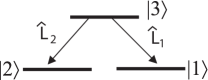
Figure 1: A simple system (a three level atom) which has two outputs due to the to lowering operators $\hat{L}_{1}$ and $\hat{L}_{2}$.

IV.1 Master equation

With no external driving [$\hat{H}=0$ in Eq. (13)], the solution of the master equation can be determined analytically. To illustrate a non-trivial solution we calculated this solution for the initial condition $|{\psi(0)}\rangle=0.4123|{1}\rangle+0.1|{2}\rangle+(0.9+0.1i)|{3}\rangle$ and coupling constants $\gamma_{1}=0.5$ and $\gamma_{2}=1$. This is shown in Fig. 2. In this figure it is observed that as time goes on, the state becomes mixed. This is seen as the purity $p(t)={\rm Tr}[\rho^{2}(t)]$ of the state decays (although not monotonically) as time increases. This figure also shows that the state becomes a mixture of the two ground states, with the ground state associated with the larger coupling constant being weighted more heavily, even though it started with less weight.

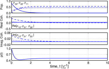
Figure 2: The solution to the master equation. The first subplot shows $\rho_{33}(t)$ (solid line), $\rho_{22}(t)$ (dashed line) and $\rho_{11}(t)$ (dotted line). The second and third subplot show the real and imaginary parts respectively of $\rho_{12}(t)$ (solid line), $\rho_{31}(t)$ (dashed line) and $\rho_{32}(t)$ (dotted line). The fourth subplot illustrates the purity of this state. This is all for the initial condition $|{\psi(0)}\rangle=0.4123|{1}\rangle+0.1|{2}\rangle+(0.9+0.1i)|{3}\rangle$ and $\gamma_{1}=0.5$ and $\gamma_{2}=1$.

IV.2 Conditional evolution: The quantum trajectory

In this section we consider the trajectory $\rho_{{\bf R}}(t)$ which occurs when output $\hat{L}_{1}$ is monitored using homodyne-$x$ detection and output $\hat{L}_{2}$ is un-monitored. A schematic of this measurement process is shown in Fig. 3. Because this arrangement is an inefficient measurement we have to use the operation defined in Eq. (5). To determine the Kraus operators we need to present the underlying dynamics in more detail. For the interaction of this system with a Markovian bath (and under the rotating wave approximation and in the interaction frame) the total Hamiltonian is

$$H(t) = i\hbar\sqrt{\gamma_{1}}\,\int\delta(t-t^{\prime})[\hat{L}_{1}\hat{b}_{r}^{\dagger}(t^{\prime})-\hat{L}_{1}^{\dagger}\hat{b}_{r}(t^{\prime})]dt^{\prime}$$

$$+i\hbar\sqrt{\gamma_{2}}\,\int\delta(t-t^{\prime})[\hat{L}_{2}\hat{b}_{f}^{\dagger}(t^{\prime})-\hat{L}_{2}^{\dagger}\hat{b}_{f}(t^{\prime})]dt^{\prime}.$$

Here $\hat{b}_{r}(t)$ and $\hat{b}_{f}(t)$ are the temporal-mode annihilation operators for the detected ($\hat{b}_{r}$) and non-detected ($\hat{b}_{f}$) fields (baths). Since these fields are Markovian there will be a commutator relationship for the field of the following form

$$[{\hat{b}_{i}(t),\hat{b}_{j}^{\dagger}(s)}]=\delta(t-s)\delta_{i,j},$$ (53)

where $i$, $j$ denotes either of the two baths. This indicates that the field operators are gaussian white noise operators. Thus they obey Itô calculus and the infinitesimal evolution operator is GarParZol92 ; GarZol00

$$\hat{U}(t+dt,t) = \exp\Big{\{}\sqrt{\gamma_{1}}\,[\hat{L}_{1}d\hat{B}_{r}^{\dagger}(t)-\hat{L}_{1}^{\dagger}d\hat{B}_{r}(t)]$$ (54)

$$+\sqrt{\gamma_{2}}\,[\hat{L}_{2}d\hat{B}_{f}^{\dagger}(t)-\hat{L}_{2}^{\dagger}d\hat{B}_{f}(t)]\Big{\}},$$

where $d\hat{B}_{i}$ satisfies the commutator relation

$$[d\hat{B}(t)_{i},d\hat{B}_{j}^{\dagger}(t)]=dt\delta_{i,j}.$$ (55)

Thus $\hat{U}(t+dt,t)$ is an operator acting in the Hilbert space ${\cal H}_{s}\otimes{\cal H}_{r}\otimes{\cal H}_{f}$, where ${\cal H}_{s}$, ${\cal H}_{r}$ and ${\cal H}_{f}$ are the Hilbert spaces for the system, detected field and non detected field respectively.

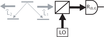
Figure 3: A schematic representing homodyne measurement of one of the outputs of the three level atom. In an ordinary homodyne measurement the signal is coupled to a classical local oscillator (LO) via a low reflective beam splitter and then detected using a photoreceiver.

Now, given that a projective measurement is made on bath field $\hat{b}_{r}(t)$ and bath field $\hat{b}_{f}(t)$ is completely unobserved the state of the system after this measurement (time $dt$ later) is given by Eqs. (1) and (5) with $T=dt$, and the Kraus operator is

$$\hat{K}_{r,f}(dt)=\langle{f}|_{f}\langle{r}|_{r}\hat{U}(t+dt,t)|{0}\rangle_{r}|{0}\rangle_{f}.$$ (56)

Here $\{|{r}\rangle_{r}\}$ is the set of orthogonal states the bath is projected into, while $\{|{f}\rangle_{f}\}$ is any arbitrary orthogonal basis set. For a homodyne-$x$ measurement of bath $\hat{b}_{r}(t)$ the set $\{|{r}\rangle_{r}\}$ corresponds to the eigenset of the operator $d\hat{B}_{r}(t)+d\hat{B}_{r}^{\dagger}(t)$ GoeGra94 and the results $r$ are the corresponding eigenvalues. Note we have assumed that initially the baths, for all the temporal-modes, are in the vacuum state.

After some simple rearrangement and using $(rdt)^{2}=dt$, the POM elements for this measurement are of the form

$$\hat{F}_{r}(dt)=|\langle{r}|{0}\rangle_{r}|^{2}[1+\sqrt{\gamma_{1}}\,r(t+dt)dt\hat{x}_{1}],$$ (57)

where $\hat{x}_{1}=\hat{L}_{1}+\hat{L}_{1}^{\dagger}$. Thus

$${P}(r,t+dt) = |\langle{r}|{0}\rangle|^{2}[1+rdt\sqrt{\gamma_{1}}\,\langle\hat{x}_{1}\rangle_{t}],$$ (58)

where $\langle\hat{x}_{1}\rangle_{t}={\rm Tr}[\hat{x}_{1}\rho(t)]$. Using the fact that $|{r}\rangle$ is a temporal-quadrature state,

$$|\langle{r}|{0}\rangle_{r}|^{2}=\sqrt{\frac{dt}{2\pi}}\,\exp\Big{(}-\frac{r^{2}}{2/dt}\Big{)},$$ (59)

we can rearrange this to

$${P}(r,t+dt)=\sqrt{\frac{dt}{2\pi}}\,\exp\Big{[}-\frac{[r-\sqrt{\gamma_{1}}\,\langle\hat{x}_{1}\rangle_{t}]^{2}}{2/dt}\Big{]}.$$ (60)

This implies that the random variable associated with this distribution, $r(t+dt)dt$, is a gaussian random variable (GRV) of mean $\sqrt{\gamma_{1}}\,\langle\hat{x}_{1}\rangle_{t}dt$ and variance $dt$. That is,

$$r(t+dt)dt=dW(t)+dt\sqrt{\gamma_{1}}\,\langle\hat{x}_{1}\rangle_{t},$$ (61)

where $dW(t)$ is a Wiener increment Gar85 .

Using the above and Eqs. (1) and (5) the stochastic master equation for this system is

$$d\rho_{\bf R}(t+dt) =dt\Big{(}\gamma_{2}{\cal D}[\hat{L}_{2}]+\gamma_{1}{\cal D}[\hat{L}_{1}]$$

$$+dW(t)\sqrt{\gamma_{1}}\,{\cal H}[\hat{L}_{1}]/dt\Big{)}\rho_{\bf R}(t),$$

where ${\cal H}[\hat{A}]$ is the superoperator

$${\cal H}[\hat{A}]\rho=\hat{A}\rho+\rho\hat{A}^{\dagger}-{\rm Tr}[\hat{A}\rho+\rho\hat{A}^{\dagger}]\rho.$$ (63)

To illustrate an example quantum trajectory, Eq. (IV.2) was solved for a randomly chosen record ${\bf R}$ and the same parameters used in Fig. 2. This is shown in Fig. 4. It is observed that this state evolution is stochastic in time and becomes mixed (but not as mixed as the average evolution). It is interesting to note that by performing this measurement the coherence $\rho_{12,{\bf R}}(t)$, which was a constant of motion for the average state, becomes comparable to the other coherence and does not decay with time.

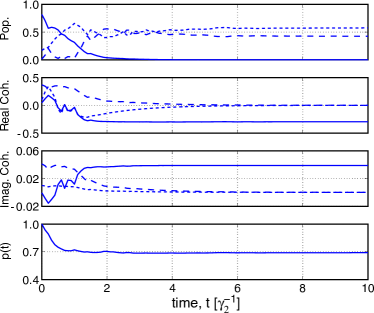
Figure 4: The solution to $\rho_{{\bf R}}$ written in matrix elements. The first subplot shows $\rho_{33,{\bf R}}(t)$ (solid line), $\rho_{22,{\bf R}}(t)$ (dashed line), $\rho_{11,{\bf R}}(t)$ (dotted line). The second and third subplot show the real and imaginary parts respectively of $\rho_{12,{\bf R}}(t)$ (solid line), $\rho_{31,{\bf R}}(t)$ (dashed line) and $\rho_{32,{\bf R}}(t)$ (dotted line). The fourth subplot illustrates the purity. We have used the same parameters as in Fig. 2

IV.3 The ostensible numerical technique

In Sec. II.3 we observed that the conditional evolution of a partly monitored system could be simulated by assuming that fictitious measurements are made on the unobservable process. For this system we assume that a fictitious homodyne-$x$ measurement is made on output $\hat{L}_{2}$. Note we could have chosen any unraveling for ${\bf F}$.

To determine the SSE for the ostensible state $|{\bar{\psi}_{{\bf R,F}}(t)}\rangle$ [the state which we substitute into Eq. (24) to determine the actual conditional evolution] we have to derive the measurement operator for the combined real and fictitious measurements, as well as make a convenient choice for $\Lambda({\bf F},{\bf R})$. Using Eq. (19) and the fact that we are performing homodyne-$x$ measurements the measurement operator is

$$\hat{M}_{r,f}(dt) = \langle{f}|0\rangle\langle{r}|0\rangle\Big{(}1+\sqrt{\gamma_{1}}\,rdt\hat{L}_{1}+\sqrt{\gamma_{2}}\,fdt\hat{L}_{2}$$ (64)

$$-\gamma_{1}dt\hat{L}_{1}^{\dagger}\hat{L}_{1}/2-\gamma_{2}dt\hat{L}_{2}^{\dagger}\hat{L}_{2}/2\Big{)},$$

where the bath states $|{f}\rangle$ and $|{r}\rangle$ are temporal quadrature states acting in Hilbert spaces ${\cal H}_{f}$ and ${\cal H}_{r}$ respectively. To derive this we have expanded Eq. (54) to first order in $dt$ and used the fact that $(fdt)^{2}=(rdt)^{2}=dt$. Since the real distribution is Gaussian (with a variance $1/dt$) a convenient choice for $\Lambda({\bf F},{\bf R})$ is $\Lambda({\bf F})\Lambda({\bf R})$ where $\Lambda({\bf F})=\Lambda(f_{k})\ldots\Lambda(f_{1})$ and $\Lambda({\bf R})=\Lambda(r_{k})\ldots\Lambda(r_{1})$ with

$$\Lambda(r) = \sqrt{\frac{dt}{2\pi}}\,\exp\Big{[}-\frac{(r-\lambda)^{2}}{2/dt}\Big{]}$$ (65)

$$\Lambda(f) = \sqrt{\frac{dt}{2\pi}}\,\exp\Big{[}-\frac{(f-\mu)^{2}}{2/dt}\Big{]}.$$ (66)

Here $\lambda$ and $\mu$ are arbitrary parameters. With these ostensible distributions, Eq. (64), and Eq. (20), the ostensible SSE is

$$d|{\bar{\psi}_{\bf R,F}(t)}\rangle = dt\Big{(}[r-\lambda](\sqrt{\gamma_{1}}\,\hat{L}_{1}-\lambda/2)+[f-\mu]$$ (67)

$$\times(\sqrt{\gamma_{1}}\,\hat{L}_{2}-\mu/2)-\mbox{$\frac{1}{2}$}[\gamma_{1}\hat{L}_{1}^{\dagger}\hat{L}_{1}+\gamma_{2}\hat{L}_{2}^{\dagger}\hat{L}_{2}$$

$$-\sqrt{\gamma_{1}}\,\lambda\hat{L}_{1}-\sqrt{\gamma_{2}}\,\mu\hat{L}_{2}+\lambda^{2}/4+\mu^{2}/4]\Big{)}$$

$$\times|{\bar{\psi}_{\bf R,F}(t)}\rangle.$$

Now since we are interested in calculating $\rho_{{\bf R}}(t)$ based on an assumed known real record ${\bf R}$, we can rewrite Eq. (67) as

$$dc_{1} = c_{3}[\sqrt{\gamma_{1}}\,(r-\lambda)dt+dt\lambda/2]-c_{1}[\sqrt{\gamma_{2}}\,d{\cal W}\mu$$ (68)

$$+\sqrt{\gamma_{1}}\,(r-\lambda)dt\lambda+dt\lambda^{2}/4+dt\mu^{2}/4]/2,$$

$$dc_{2} = c_{3}[\sqrt{\gamma_{2}}\,d{\cal W}+dt\mu/2]-c_{2}[\sqrt{\gamma_{2}}\,d{\cal W}\mu$$ (69)

$$+\sqrt{\gamma_{1}}\,(r-\lambda)dt\lambda+dt\lambda^{2}/4+dt\mu^{2}/4]/2$$

$$dc_{3} = c_{3}[-\gamma dt+\sqrt{\gamma_{2}}\,d{\cal W}\mu+\sqrt{\gamma_{1}}\,(r-\lambda)dt\lambda$$ (70)

$$+dt\lambda^{2}/4+dt\mu^{2}/4]/2,$$

where $\gamma=\gamma_{1}+\gamma_{2}$. Here we have used the identity

$$|{\bar{\psi}(t)}\rangle=c_{1}|{1}\rangle+c_{2}|{2}\rangle+c_{3}|{3}\rangle,$$ (71)

and replaced $fdt$ with $d{\cal W}(t)+\mu dt$, where $d{\cal W}(t)$ is a Wiener increment.

To illustrate the convergence of our method the ensemble average of the above ostensible SSE for $\lambda=\mu=0$ was calculated for $n=10$ and $n=1000$. To quantify how closely the ensemble method reproduces $\rho_{{\bf R}}(t)$ we used the fidelity measure, which for two different quantum states is defined as

$$F^{\rm(Q)}(t)={\rm Tr}[\sqrt{\sqrt{\rho_{1}(t)}\,\rho_{2}(t)\sqrt{\rho_{1}(t)}\,}\,].$$ (72)

Note this measure ranges from 0 to 1 with 0 indicating two orthogonal states and 1 indicating the same state. The result of this measure for the actual $\rho_{{\bf R}}(t)$ and the ensemble version are shown in part A of figure 5. Here we see that for larger ensemble size the fidelity is closer to one, indicating that as we increase the ensemble size our ostensible method approaches the actual $\rho_{{\bf R}}(t)$.

To illustrate the effect of choosing different ostensible distributions we considered the case when $\lambda=0$ and

$$\mu=\sqrt{\gamma_{2}}\,\frac{\langle{\bar{\psi}_{\bf R,F}(t)}|\hat{L}_{2}+\hat{L}_{2}^{\dagger}|{\bar{\psi}_{\bf R,F}(t)}\rangle}{\langle{\bar{\psi}_{\bf R,F}(t)}|\bar{\psi}_{\bf R,F}(t)\rangle}.$$ (73)

That is, the ostensible probability for the $k^{th}$ fictitious results is the true probability we would expect based on the past real and fictitious results up to, but not including the time $kdt$. The motivation for this choice is that with $\mu=0$, the improbable trajectories, ones that tend towards being inconsistent with the full real record, will have norms that are very small and as such have little contribution to the ensemble average. By contrast, using Eq. (73), the improbable trajectories are less likely to be generated, so avoiding useless simulations. With this ostensible distribution the fidelity measure was calculated for $n=10$ and $n=1000$. These results are shown in part $B$ of figure 5. Here we see that for the smaller ensemble size the fidelity is closer to one than that observed using the first ostensible case. This indicates that the rate of convergence for this case is greater than the $\lambda=\mu=0$ case.

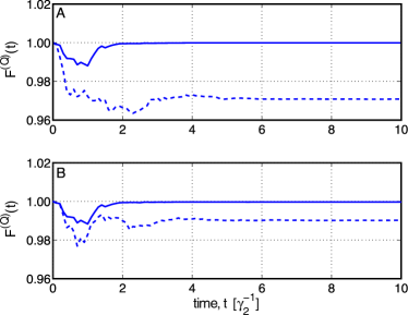
Figure 5: This figure shows the fidelity between the actual $\rho_{{\bf R}}(t)$ and our ensemble method for ensembles sizes 10 (dotted) and 1000 (solid). Part $A$ corresponds to a linear ostensible distribution while part $B$ refers to the non-linear ostensible distribution. The same parameters were used as in Fig. 2.

V A Classical system with an internal unobserved process

In this section we consider continuous-in-time measurements with Gaussian precision of a classical system driven by an unobservable noise process. This for example could correspond to a measurement of the voltage across a resistor that is driven by a noisy classical current.

V.1 The average evolution

We restrict ourselves to unconditional state evolution described by the Fokker Plank equation Eq. (41). This equation has as its solution a distribution that diffuses and drifts though time. Using Eq. (34) and only considering one interval in time we can write

$$P(x^{\prime},t+dt)=\int dx{\cal O}(x^{\prime},t+dt|x,t)P(x,t),$$ (74)

which when compared to Eq. (41) implies that RHS of the above equation equals

$$\int dx[1-dt\partial_{x^{\prime}}A(x,t)+dt\partial^{2}_{{x^{\prime}}}D^{2}(x,t)/2]\delta(x^{\prime}-x)$$

$$\times P(x,t).$$ (75)

By introducing an arbitrary Gaussian distribution $P(f,t+dt)$ with mean $m(t)$ and variance $1/dt$, that is

$$P(f,t+dt)=\sqrt{\frac{dt}{2\pi}}\,\exp\Big{[}-\frac{[f-m(t)]^{2}}{2/dt}\Big{]},$$ (76)

Eq. (V.1) can be rewritten as

$$\int dfP(f,t+dt)\int dx[1-dt\partial_{x^{\prime}}A(x,t)-dt[f-m(t)]$$

$$\times\partial_{x^{\prime}}D_{f}(x,t)+dt\partial^{2}_{{x^{\prime}}}D^{2}(x,t)/2]\delta(x^{\prime}-x)P(x,t).$$

By using Itô calculus and a Taylor expansion this can be rewritten as

$$\int dx{\rm E}_{f}\Big{\{}\delta[x^{\prime}-x-dtA(x,t)-dt[f(t+dt)-m(t)]$$

$$\times D(x,t)]\Big{\}}P(x,t).$$ (78)

where $f(t+dt)dt=m(t)dt+d{\cal W}(t)$. Thus

$${\cal O}(x^{\prime},t+dt|x,t)={\rm E}_{f}\Big{\{}\delta[x^{\prime}-x_{f}(t+dt)]\Big{\}},$$ (79)

where $x_{f}(t+dt)$ is determined by the following SDE

$$dx_{\bf F}(t)=dtA[x_{\bf F}(t),t]+dt[f(t+dt)-m(t)]D[x_{\bf F}(t),t].$$ (80)

Note here we have written the SDE for the complete record ${\bf F}$.

V.2 Conditional evolution: The Kushner-Stratonovich equation

To derive the KSE we start by deriving ${\cal O}_{r}(x^{\prime},t^{\prime}|x,t)$ and $P(r,t+dt)$. For the case when the classical measurement has a back action that is independent of the result $r(t+dt)$, the operation for the measurement is given by

$${\cal O}_{r}(x^{\prime},t^{\prime}|x,t)={\cal O}(x^{\prime},t^{\prime}|x,t)P(r,t|x,t),$$ (81)

where ${\cal O}(x^{\prime},t^{\prime}|x,t)=B(x^{\prime},t^{\prime}|x,t)$. Thus to derive ${\cal O}_{r}(x^{\prime},t^{\prime}|x,t)$ we need only $P(r,t|x,t)$. For a measurement that has a precision limited by Gaussian white noise it follows that

$$P(r,t|x,t)=F_{r}(x,t)=\frac{\sqrt{dt}}{\sqrt{2\pi\beta}}\exp[-(r-x)^{2}dt/2\beta],$$ (82)

where $\beta$ is a constant characterizing the classical measurement strength.

To find $P(r,t)$ we substitute Eq. (82) into Eq. (32). This gives

$$P(r,t+dt)=\int dx\frac{\sqrt{dt}}{\sqrt{2\pi\beta}}\exp[-(r-x)^{2}dt/2\beta]P(x,t).$$ (83)

After some simple stochastic algebra and using $r^{2}=\beta/dt$ this can be simplified to WarWis03a

$$P(r,t+dt)=\frac{\sqrt{dt}}{\sqrt{2\pi\beta}}\exp[-(r-\langle x\rangle_{t})^{2}dt/2\beta],$$ (84)

where for the classical system $\langle x\rangle_{t}=\int xP(x,t)dx$. From Eq. (84) the stochastic representation of $r(t+dt)$ is a Gaussian random variable with mean $\langle x\rangle_{t}$ and variance $\beta dt$. That is,

$$r(t+dt)=\langle x\rangle_{t}+\sqrt{\beta}dW(t)/dt.$$ (85)

With all the above information and Eq. (30) the conditional state at time $t^{\prime}=t+dt$ is

$$P_{r}(x^{\prime},t+dt)=\int dx{\rm E}_{f}\Big{\{}\delta[x^{\prime}-x_{f}(t+dt)]\Big{\}}\Big{\{}1$$

$$+[x-\langle x\rangle_{t}][r-\langle x\rangle_{t}]dt/\beta\Big{\}}P(x,t).$$ (86)

Here we have expanded the exponentials in Eq. (84) and Eq. (82) to second order in $dt$ and used $r^{2}=\beta/dt$. Taylor expanding the delta function and averaging over the $f(t+dt)$ [using Eq. (76)] for each step in time gives the KSE

$$P_{\bf R}(x,t+dt) = P_{\bf R}(x,t)+dt[x-\langle x\rangle_{t}][r(t+dt)-\langle x\rangle_{t}]$$ (87)

$$\times P_{\bf R}(x,t)/\beta-dt\partial_{x}[{A}({x},t)P_{\bf R}(x,t)]$$

$$+\mbox{$\frac{1}{2}$}dt\partial^{2}_{x}[D^{2}({x},t)P_{\bf R}(x,t)]$$

and $\langle x\rangle_{t}$ becomes $\int xP_{\bf R}(x,t)dx$. In general to solve this equation we need to solve for all $x$. For some ${A}({x},t)$ and $D(x,t)$ this can be a rather lengthy numerical problem. In the following section we will present our ostensible technique which allows us to reformulate the problem to solving two coupled SDEs, at the cost of performing an ensemble average.

V.3 The ostensible numerical technique

As shown in Sec. III.3, if we consider the unobservable process ${\bf F}$ as actually occurring then we can simulate the KSE by using Eq. (49), and $\bar{P}_{{\bf R},{\bf F}}(x,t)$ is determined by solving two coupled SDEs. For the case when the classical measurement has Gaussian precision and the back action only depends on the white noise process $f(t)$, we can rewrite $P(f,t^{\prime};r,t|x,t)$ in Eq. (51) as $P(f,t^{\prime})P(r,t|x,t)$ where $P(f,t^{\prime})$ is given by Eq. (76) and $P(r,t|x,t)$ is given by Eq. (82). Thus $\dot{x}_{\bf R,F}(t)$ becomes $\dot{x}_{\bf F}(t)$ and is given by Eq. (80). To find the differential equation for $\dot{p}_{\bf R,F}(t)$ we need to assume a form for the ostensible distribution $\Lambda(f,r)$. We use $\Lambda(f,r)=\Lambda(f)\Lambda(r)$, where

$$\Lambda(r) = \sqrt{\frac{dt}{2\pi}}\,\exp\Big{[}-\frac{(r-\lambda)^{2}}{2\beta/dt}\Big{]}$$ (88)

and $\Lambda(f)$ is given by Eq. (66). Extending Eq. (51) to continuous measurements gives

$$dp_{\bf R,F}(t) = dt[m(t)-\mu][f(t+dt)-\mu]p_{\bf R,F}(t)$$

$$+dt[x(t)-\lambda][r(t+dt)-\lambda]p_{\bf R,F}(t)/\beta.$$

Thus to determine $\bar{P}_{\bf R,F}(x,t)$ we only need to simulate Eqs. (80) and (V.3) with ${\bf R}$ assumed known and $f(t+dt)$ given by Eq. (66). $P_{\bf R}(x,t)$ is then determined by Eq. (47). Since the theory requires $\bar{P}_{\bf R,F}(x,t)$ to be a delta function, one might conclude that this method is only valid for initial conditions of the form ${P}(x,0)\rho(0)=\delta(x-x_{0})$. Infact, we are not limited to this case. To consider other initial conditions we simply choose the initial value $x_{0}$ in Eq. (80) from the distribution ${P}(x,0)$.

V.4 A simple example

To illustrate the classical theory we consider a Gaussian measurement of a classical system that is driven by an an unobservable white noise process with $m(t)=0$ and drift and diffusion functions given by

$$A({x},t) = -kx+l,$$ (90)

$$D({x},t) = b.$$ (91)

If this is the case then $P_{{\bf R}}(x,t)$ has a Gaussian solution with a mean $\langle x_{\bf R}\rangle_{t}$ and variance $\nu_{\bf R}(t)$ given by

$$d\langle x_{\bf R}\rangle_{t} = dt\{\nu_{\bf R}(t)[r(t+dt)-\langle x_{\bf R}\rangle_{t}]/\beta-k\langle x_{\bf R}\rangle_{t}$$ (92)

$$+l\},$$

$$d\nu_{\bf R}(t) = dt[-\nu_{\bf R}^{2}(t)/\beta-2k\nu_{\bf R}(t)+b^{2}],$$ (93)

and $r(t+dt)=\langle x_{\bf R}\rangle_{t}+dW(t)$. That is, as time increases the measurement has the effect of reducing the variance but the diffusive coefficient $b$ causes this variance to increase. The mean, however contains both the deterministic evolution and a random term due the measurement. To illustrate this solution we have simulated Eqs. (92) and (93) for the case when $A(x,t)=1-x$, $D=1$ and $\beta=1$. The results of this simulation are shown in Fig. 6 as a solid line. Here we see that the mean follows some stochastic path conditioned on the record ${\bf R}$, while the variance follows a smooth function.

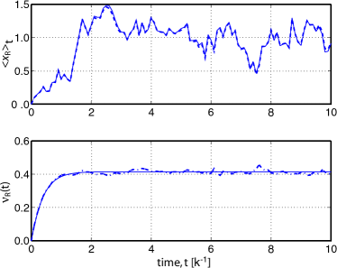
Figure 6: The mean and variance of ${P}_{{\bf R}}(x,t)$ when $\beta=1$, $A=1-x$ and $D=1$ for both ${P}_{{\bf R}}(x,t)$ calculated exactly (solid) and via the linear method for an ensemble size of 10 000 (dotted).

To illustrate our ostensible method we use the above record and solve numerically Eqs. (80) and (V.3) with $\lambda=\mu=0$. The mean and variance is then found via

$$\langle x_{\bf R}\rangle_{t} = \frac{{\rm E}_{\bf F}\Big{[}{x}_{\bf F}(t)p_{\bf R,F}(t)\Big{]}}{{\rm E}_{\bf F}\Big{[}p_{\bf R,F}(t)\Big{]}}$$ (94)

$$\nu_{\bf R}(t) = \frac{{\rm E}_{\bf F}\Big{[}x_{\bf F}^{2}(t)p_{\bf R,F}(t)\Big{]}}{{\rm E}_{\bf F}\Big{[}p_{\bf R,F}(t)\Big{]}}-\langle x_{\bf R}\rangle^{2}_{t}$$

where ${\rm E}_{\bf F}$ denotes an ensemble average over all possible fictitious records. The numerical values for the mean and variance are shown in Fig. 6 (dotted) for an ensemble size of 10 000. To get an indication of the numerical error in the solution from our method, the difference from the exact solution is shown in Fig. 7. The dotted line corresponds to an ensemble of 100 and the solid to one of 10 000. Here we see that the ostensible method solution agrees well with the exact solution and as we increase the ensemble size the difference between these solutions decreases. To get a better indication of how well our method reproduces the actual ${P}_{{\bf R}}(x,t)$, we also calculated the classical fidelity, which is defined by

$$F^{(C)}(t)=\int dx\sqrt{P_{1}(x,t)}\,\sqrt{P_{2}(x,t)}\,.$$ (96)

This was calculated under the assumption that the state calculated via the ostensible method was also Gaussian. This is illustrated in Fig. 7, where we see that for the larger ensemble the fidelity is very close to one, implying that the distributions are almost identical.

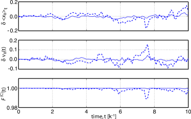
Figure 7: The first and second plot show the difference between the mean and variance of ${P}_{{\bf R}}(x,t)$ calculated by the linear method and the know result for ensemble sizes 100 (dotted) and 10 000 (solid). The third plot shows the Fidelity between ${P}_{{\bf R}}(x,t)$ calculated by the linear method and the know result for ensemble sizes 100 (dotted) and 10 000 (solid). The parameters are the same as in Fig. 6.

VI An unobservable quantum system driving a Classical system

In this section we consider the following situation: a quantum system is monitored continuously in time by a classical system. This in turn is measured with Gaussian precision, and these are the only results to which we have access. This for example occurs when the signal from the quantum system enters a detector with a bandwidth $B$, resulting in the state of the detector being related to ${\bf F}$ by WarWis03a

$$x(t)=\int_{-\infty}^{t}dsB\exp[-B(t-s)]{f}(s).$$ (97)

Thus in a measurement that reveals $x(t)$ with perfect precession [eg $F_{r}(x)=P(r,t|x,t)=\delta(r-x)$] we could determine ${\bf F}$ (the quantum signal) by inverting the convolution in Eq. (97). But if this measurement has Gaussian precision [Eq. (82)] then we must treat the state of the detector as a classical probability distribution and use a mixture of CMT and QMT to describe the conditional state of the supersystem (classical and quantum system). To denote the supersystem we use the notation $\rho(x,t)$, where $x$ refers to the classical configuration space and $\rho$ denotes an object acting on a Hilbert space. This has the interpretation whereby $P(x,t)={\rm Tr}[\rho(x,t)]$ is the (marginal) classical state and $\rho(t)=\int\rho(x,t)dx$ is the (reduced) quantum state. For uncorrelated quantum and classical states, $\rho(x,t)=P(x,t)\rho(t)$.

VI.1 Conditional evolution

We denote the state of the supersystem conditioned on the classical result $r$ at time $t+dt$ as $\rho_{r}(x,t+dt)$. Assuming that the quantum system is not affected by the classical system, this can be expanded as

$$\rho_{r}(x,t+dt)=\sum_{f}P_{r}(f,t+dt)P_{r,f}(x,t+dt)\rho_{f}(t+dt),$$ (98)

where $\rho_{f}(t+dt)$ is the state that an observer who had access to all the quantum information would ascribe to the quantum system. That is, $f(t+dt)$ can be regarded as really existing (with the collapse of the wavefunction occurring at this level); it is just that the real observer does not have access to this information. The state of knowledge of this real observer is different from, but consistent with, that of the hypothetical observer who has access to F.

In terms of the operation of the measurement, the conditional state can be written as

$$\rho_{r}(x^{\prime},t+dt) = \frac{\tilde{\rho}_{r}(x^{\prime},t+dt)}{P(r,t+dt)},$$ (99)

where

$$\tilde{\rho}_{r}(x^{\prime},t+dt) = \int dx\sum_{f}{\cal J}_{r,f}(x^{\prime},t+dt|x,t)$$ (100)

$$\times\hat{\cal O}_{f}(t+dt,t)\rho(x,t)/P(f,t+dt)\hskip 22.76228pt$$

and

$$P(r,t+dt) = \int dx^{\prime}{\rm Tr}\Big{[}\tilde{\rho}_{r}(x^{\prime},t+dt)\Big{]}.$$ (101)

The quantum part of the operation of measurement in defined by Eq. (5) and the classical part is defined in Eq. (36) with the replacement of $P(f,t^{\prime};r,t|x,t)\rightarrow P(f,t^{\prime})P(r,t|x,t)$ because in this system the quantum signal does not depend on the classical state.

To illustrate the above we consider the case when we are monitoring with Gaussian precision the classical system defined by Eq. (97) which is in turn monitoring the $x$ quadrature flux coming from a classically driven two level atom (TLA). This is the same as the system considered in Ref WarWis03a and as such we will simply list the important equations. The quantum part of operation is given by $\hat{\cal O}_{f}(t+dt,t)=\hat{\cal J}[\hat{M}_{f}(dt)]$ where

$$\hat{M}_{f}(dt)=\langle{f}|0\rangle[1-dt(i\hat{H}-\sqrt{\gamma}\,f\hat{\sigma}+\gamma\hat{\sigma}^{\dagger}\hat{\sigma}/2)].$$ (102)

The fictitious quantum signal statistic obeys

$$P(f,t+dt)=\int dx{\rm Tr}[\hat{\cal O}_{f}(t+dt,t)\rho(x,t)],$$ (103)

which for a homodyne-$x$ measurement can be shown to be of the form displayed in Eq. (76) with $m(t)=\sqrt{\gamma}\,{\rm Tr}[(\hat{\sigma}+\hat{\sigma}^{\dagger})\rho(t)]$. Here $\hat{\sigma}$ is the lowering operator for the TLA and $\gamma$ is the decay rate. Note here we have assumed all the quantum signal is fed into the classical system, if we wanted to simulate some inefficiency we would simply use the Kraus represention, and for the case where this inefficiency is a constant, $\eta$, we simply replace $\sigma$ in the above equations by $\sqrt{\eta}\,\sigma$.

As shown in Sec. V for a classical measurement with Gaussian precision and a back action that does not depend on the results of the measurement, the classical part of the operation is

$${\cal J}_{r,f}(x^{\prime},t+dt|x,t)=\delta[x^{\prime}-x_{f}(t+dt)]P(f,t+dt)P(r,t|x,t),$$ (104)

where $P(r,t|x,t)$ is defined in Eq. (82) and $x_{f}(t+dt)$ is given by Eq. (80). For the system we are considering, to find $A(x,t)$ and $D(x,t)$ we simply differentiate Eq. (97) and equate this with Eq. (80). Doing this gives

$$A(x,t) = -Bx+Bm(t),$$ (105)

$$D(x,t) = B.$$ (106)

Combining the quantum and classical parts of the operation and using the same techniques as in Sec. V.2 allows us to rewrite Eq. (99) for continuous-in-time measurements as

$$d\rho_{\bf R}(x,t) = dt\Big{(}B\partial_{x}x+\mbox{$\frac{1}{2}$}B^{2}\partial^{2}_{x}+\hat{\cal L}\Big{)}\rho_{\bf R}(x,t)$$ (107)

$$+dt\Big{(}\frac{[x-\langle x_{\bf R}\rangle_{t}][r(t+dt)-\langle x_{\bf R}\rangle_{t}]}{\beta}\Big{)}\rho_{\bf R}(x,t)$$

$$-dt\sqrt{\gamma}\,\partial_{x}B[\hat{\sigma}\rho_{\bf R}(x,t)+\rho_{\bf R}(x,t)\hat{\sigma}^{\dagger}],$$

where $\langle x_{\bf R}\rangle_{t}=\int x{\rm Tr}[\rho_{\bf R}(x,t)]dx$ and

$$r(t+dt)dt=\langle x_{\bf R}\rangle_{t}dt+\sqrt{\beta}\,dW(t).$$ (108)

This equation (107) has been labeled the Superoperator-Kushner-Stratonovich equation WarWis03a and represents the evolution of the combined supersystem. The first line contains the free evolution for both the quantum and the classical systems. For this quantum system

$$\hat{\cal L}[\hat{\sigma}]\rho=\frac{-i\Omega}{2}[\hat{\sigma}_{x},\rho]+\gamma\hat{\cal D}[\hat{\sigma}]\rho,$$ (109)

where $\Omega$ is the Rabi frequency and $\hat{\cal D}$ is the damping superoperator and is defined in Eq. (14). The second line of Eq. (107) describes the gaining of knowledge about the state of classical system via Gaussian measurements. Lastly the third line describes the coupling of the quantum and classical system.

For a TLA we can write the state of the supersystem as

$$\rho(x,t)=\mbox{$\frac{1}{2}$}[P(x,t)\hat{1}+X(x,t)\hat{\sigma}_{x}+Y(x,t)\hat{\sigma}_{y}+Z(x,t)\hat{\sigma}_{z}].$$ (110)

Note that $P(x,t)$ is the marginal state of knowledge for the classical system (found via tracing out the quantum degrees of freedom). Substituting this into Eq. (107) gives the following four coupled partial differential equations

$$\dot{P}_{\bf R} = [x-\langle x_{\bf R}\rangle_{t}][r-\langle x_{\bf R}\rangle_{t}]P_{\bf R}/\beta+B\partial_{x}[xP_{\bf R}$$ (111)

$$-\sqrt{\gamma}\,X_{\bf R}]+\mbox{$\frac{1}{2}$}B^{2}\partial_{x}^{2}P_{\bf R}$$

$$\dot{X}_{\bf R} = [x-\langle x_{\bf R}\rangle_{t}][r-\langle x_{\bf R}\rangle_{t}]X_{\bf R}/\beta+\mbox{$\frac{1}{2}$}B^{2}\partial_{x}^{2}X_{\bf R}$$ (112)

$$+B\partial_{x}[xX_{\bf R}-\sqrt{\gamma}\,P_{\bf R}-\sqrt{\gamma}\,Z_{\bf R}]-\mbox{$\frac{1}{2}$}\gamma X_{\bf R}$$

$$\dot{Y}_{\bf R} = [x-\langle x_{\bf R}\rangle_{t}][r-\langle x_{\bf R}\rangle_{t}]Y_{\bf R}/\beta+B\partial_{x}[xY_{\bf R}]$$ (113)

$$+\mbox{$\frac{1}{2}$}B^{2}\partial_{x}^{2}Y_{\bf R}-\Omega Z_{\bf R}-\mbox{$\frac{1}{2}$}\gamma Y_{\bf R}$$

$$\dot{Z}_{\bf R} = [x-\langle x_{\bf R}\rangle_{t}][r-\langle x_{\bf R}\rangle_{t}]Z_{\bf R}/\beta+B\partial_{x}[xZ_{\bf R}$$

$$+\sqrt{\gamma}\,X_{\bf R}]+\mbox{$\frac{1}{2}$}B^{2}\partial_{x}^{2}Z_{\bf R}+\Omega Y_{\bf R}-\gamma(P_{\bf R}+Z_{\bf R}).$$

To determine the state of knowledge for the quantum system we simply integrate out the classical degrees of freedom.

To illustrate a trajectory for this supersystem the following parameters were used; $\beta=0.5$, $B=2$, $\gamma=1$ and $\Omega=5$. The results are shown in Fig. 8 (solid line) for a randomly chosen record ${\bf R}$. This figure displays the mean and the variance of the classical trajectory found via tracing over the quantum degrees of freedom as well as the quantum state in Bloch representation after we have integrated out the classical degrees of freedom.

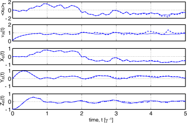
Figure 8: ${\rho}_{{\bf R}}(x,t)$ calculated via numerical integration (solid) and via the ostensible method for an ensemble size of 10 000 (dotted). The parameters are $\beta=0.5$, $B=2$, $\gamma=1$ and $\Omega=5$ and initial conditions ${\rho}(x,0)=P(x)|{g}\rangle\langle{g}|$ where $P(x)$ is a Gaussian with mean zero and variance 0.1.

VI.2 Fictitious trajectories: The ostensible numerical technique

In the above section we observed that to be able to calculate the supersystem trajectory we needed to solve four coupled partial differential functions (each involving derivatives with respect to a classical configuration coordinate $x$). This is a rather lengthy calculation which for higher dimensional ($d$) quantum systems will require $d^{2}$ partial differential equations. Here we present our linear method that allows us to reduce the problem to $d+2$ couple differential equations. The expense, again, is that an ensemble average must be performed.

To do this we simply note that we can define the following quantum and classical states

$$\bar{\rho}_{f}(t+dt)=\frac{\hat{\cal O}_{f}(t+dt,t)\rho(t)}{\bar{\Lambda}(f)}$$ (115)

and

$$\bar{P}_{r,f}(x^{\prime},t+dt)=\frac{\int dx\bar{\cal O}_{r,f}(x^{\prime},t+dt|x,t)P(x,t)}{\Lambda(f)\Lambda(r)},$$ (116)

where

$$\bar{\cal O}_{r,f}(x^{\prime},t+dt|x,t)=\delta[x^{\prime}-x_{f}(t+dt)]P(r,t|x,t)\bar{\Lambda}(f).$$ (117)

Note the bar above $\bar{\Lambda}(f)$ means that the ostensible distribution used to scale the quantum state does not have to be the same as that used to scale the classical state. Here for simplicity we consider only the case when they are the same (as no numerical advantage is gain by different choices). Using the above equations we can rewrite Eqs. (99) and (101) as

$$\rho_{r}(x^{\prime},t+dt) = \frac{\sum_{f}\Lambda(f)\Lambda(r)\bar{P}_{r,f}(x^{\prime},t+dt)\bar{\rho}_{f}(t+dt)}{P(r,t+dt)},$$

$$P(r,t+dt) = \int dx\sum_{f}{\rm Tr}[\Lambda(f)\Lambda(r)\bar{P}_{r,f}(x,t+dt)$$ (119)

$$\times\bar{\rho}_{f}(t+dt)].$$

Thus to simulate $\rho_{\bf R}(x,t)$ we need only to calculate $\bar{P}_{\bf R,F}(x,t)$ and $\bar{\rho}_{\bf F}(t)$ for a specific record ${\bf R}$.

For the above TLA-classical detector system with $\Lambda(r)$ and $\Lambda(f)$ defined by Eqs. (88) and (66) respectively, $\bar{P}_{\bf R,F}(x^{\prime},t)$ has a solution of the form $p_{\bf R}(t)\delta[x^{\prime}-x_{\bf R,F}(t)]$ where $x_{\bf F}(t)$ is given by

$$d{x}_{\bf F}(t)=dt[-Bx_{\bf F}(t)+Bf(t+dt)]$$ (120)

and $p_{\bf R,F}(t)$ is given by

$$dp_{\bf R,F}(t)=dt[x_{\bf F}(t)-\lambda][r(t+dt)-\lambda]p_{\bf R,F}(t)/\beta,\hskip 28.45274pt.$$ (121)

Thus we can rewrite Eq. (VI.2) as

$$\rho_{\bf R}(x,t)=\frac{{\rm E}_{\bf F}\Big{[}\delta[x-x_{\bf F}(t)]p_{\bf R,F}(t)\bar{\rho}_{\bf F}(t)\Big{]}}{{\rm E}_{\bf F}\Big{[}p_{\bf R,F}(t)\check{p}_{\bf F}(t)\Big{]}},$$ (122)

where $\check{p}_{\bf F}(t)={\rm Tr}[\bar{\rho}_{\bf F}(t)]$.

To determine the evolution of the ostensible quantum state we simply substitute the measurement operator defined in Eq. (102) with $\hat{H}=\Omega\hat{\sigma}_{x}/2$ and the ostensible distribution ${\Lambda}(f)$ into Eq. (115). Doing this gives

$$d\bar{\rho}_{\bf F}(t) = dt\frac{-i\Omega}{2}[\hat{\sigma}_{x},\rho_{\bf F}(t)]+dt\gamma\hat{\cal D}[\hat{\sigma}]\rho_{\bf F}(t)+$$ (123)

$$dt[f(t+dt)-{\mu}][\sqrt{\gamma}\,\hat{\sigma}\rho_{\bf F}(t)$$

$$+\sqrt{\gamma}\,\rho_{\bf F}(t)\hat{\sigma}^{\dagger}-{\mu}\rho_{\bf F}(t)].$$

However since we have assumed that all the quantum signal is fed into the detector the evolution of the ostensible quantum state can be written as an ostensible SSE. That is,

$$d|{\bar{\psi}_{\bf F}(t)}\rangle = dt\Big{(}-\frac{i\Omega}{2}\hat{\sigma}_{x}+[f(t+dt)-\mu](\sqrt{\gamma}\,\hat{\sigma}-\mu/2)$$ (124)

$$-\mbox{$\frac{1}{2}$}[\gamma\hat{\sigma}^{\dagger}\hat{\sigma}-\sqrt{\gamma}\,\mu\hat{\sigma}+\mu^{2}/4]\Big{)}|{\bar{\psi}_{\bf F}(t)}\rangle.\hskip 22.76228pt$$

Thus to determine $\rho_{\bf R}(x,t)$ all we need to do is solve the above SSE and Eqs. (120) and (121) for ${\bf R}$ assumed known and $f(t+dt)dt=d{\cal W}+dt\mu$ where $d{\cal W}$ is a Wiener increment. Once solved the quantum state conditioned on ${\bf R}$ is given by

$${\chi}_{\bf R}(t) = \frac{{\rm E}_{\bf F}\Big{[}p_{\bf R,F}(t)\check{\chi}_{\bf F}(t)\Big{]}}{{\rm E}_{\bf F}\Big{[}p_{\bf R,F}(t)\check{p}_{\bf F}(t)\Big{]}},$$ (125)

where ${\chi}_{i}=\{\check{x}_{i},\check{y}_{i},\check{z}_{i}\}$ are the Bloch vectors of the quantum state. The moments of the classical state are given by

$$\langle x^{m}_{\bf R}\rangle_{t} = \frac{{\rm E}_{\bf F}\Big{[}{x}^{m}_{\bf F}(t)p_{\bf R,F}(t)\check{p}_{\bf F}(t)\Big{]}}{{\rm E}_{\bf F}\Big{[}p_{\bf R,F}(t)\check{p}_{\bf F}(t)\Big{]}}.\hskip 14.22636pt$$ (126)

To illustrate this method we considered two choices for the ostensible distributions. The first is $\lambda=\mu=0$; that is, all the ostensible distributions are Gaussian distributions of mean zero and variance $dt$. The second case corresponds to the situation when $\lambda=0$ and $\mu=\sqrt{\gamma}\,{\rm Tr}[(\hat{\sigma}+\hat{\sigma}^{\dagger})\rho_{\bf F}(t)]$; that is, the fictitious distribution is treated as the real unobservable distribution. Both cases were simulated to show the robustness of our numerical technique and to demonstrate that while any ostensible distributions can be chosen a more realistic choice will result in a faster convergence. To demonstrate this we numerically solved Eq. (107) and used this as our reference solution. Then we compared the mean and variance of the classical marginal states and the fidelity for quantum reduced states (using Eq. (72) once the classical space has been removed) for both ostensible cases and with ensemble sizes of 100 and 10 000. These results are shown Fig. 9 where it is observed that for the larger ensemble size the difference in the classical marginal state is small and the quantum fidelity is close to one, indicating that our ostensible method has reproduced the known result and is converging. Furthermore it is observed that for the second case for the same ensemble size this difference is smaller thereby indicating that the second method convergence is faster.

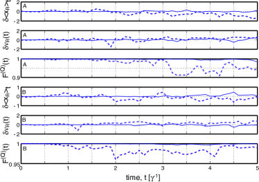
Figure 9: This figure shows the quantum and classical fidelity between the actual solution and our ostensible solution for ${\rho}_{{\bf R}}(x,t)$. Part A corresponds to the $\lambda=\mu=0$ case while part B represents the $\lambda=0$ and $\mu=\sqrt{\gamma}\,{\rm Tr}[(\hat{\sigma}+\hat{\sigma}^{\dagger})\rho_{\bf F}(t)]$ case. In both case an ensemble size of $n=100$ (dotted) and $n=10000$ (solid) was used. The system parameters are the same as in Fig. 8.

VII Discussion and Conclusion

The central topic of this paper was to investigate the conditional dynamics of partially observed systems (classical and quantum). Due to the fact that the information obtained is incomplete we have to assign a mixed state to the system. For a quantum system this means the state of knowledge given result $r$ is given by the state matrix $\rho_{r}(t)$ and for a classical system a probability distribution $P_{r}(x,t)$ has to be used. If we consider a joint system (for example a classical detector is used to monitor a quantum system) the conditional state is given by $\rho_{r}(x,t)$.

Even when we consider continuous-in-time monitoring we can still have incomplete information because of unobserved processes. For this case the conditional state trajectories obey either a stochastic master equation (for a quantum system), a Kushner Stratonovich equation (for a classical system) or a superoperator Kushner-Stratonovich equation (for the joint system). That is, to simulate the conditional state we have to solve a rather numerically expensive equation. In this paper we showed that by introducing a fictitious record ${\bf F}$ for the unobserved processes and ostensible measurement theory we can reduce this problem to solving pure states (stochastic Schrödinger   equations for the quantum system or stochastic differential equations for the classical system) conditioned on both ${\bf R}$ and ${\bf F}$. Then by averaging over all possible ${\bf F}$ we get the require conditional state. That is the numerical memory requirements are decreased by a factor of $N$, the number of basis states for the system. However, this is at the cost of an ensemble average.

In summary, our ostensible method will be useful for investigating realistic situations where the dimensions of the systems are large. It is also much easier to implement numerically than the standard technique, so we expect it to find immediate applications.

Appendix A Why it is necessary to use the ostensible method

To show that we must use an ostensible distribution rather then the real distribution, for our numerical technique, we consider two consecutive measurements. The state of the system (which we take to be quantum for specificity) after these two measurement is

$$\rho_{r_{2},r_{1}} = \sum_{f_{2},f_{1}}P(f_{2},f_{1}|r_{2},r_{1})\rho_{r_{2},f_{2},r_{1},f_{1}}$$ (127)

$$= \frac{\sum_{f_{2},f_{1}}\hat{\cal J}[\hat{M}_{f_{2},r_{2}}\hat{M}_{f_{1},r_{1}}]\rho(0)}{P(r_{1},r_{2})}.$$

This can be rewritten as

$$\rho_{r_{2},r_{1}}=\sum_{f_{2},f_{1}}\frac{\hat{\cal J}[\hat{M}_{f_{2},r_{2}}]\hat{\cal J}[\hat{M}_{f_{1},r_{1}}]\rho(0)}{P(r_{2},f_{2}|r_{1},f_{1})P(r_{1},f_{1})}\frac{P(r_{2},f_{2},r_{1},f_{1})}{P(r_{1},r_{2})}.$$ (128)

The first term can be viewed as the part that determines the trajectory and the second term as the part which determines the weighting factor for this trajectory. Considering only the weighting factor we can rewrite this as $P(f_{2},f_{1}|r_{2},r_{1})$, which, unless we have the full numerical solution, is not determinable. To be more specific we cannot separate this term into $P(f_{1})P(f_{2}|f_{1},r_{1})$ and thus we cannot create a trajectory that steps through time with the correct statistics for $f_{k}$.

However by introducing an ostensible distribution we can rewrite Eq. (128) as

$$\rho_{r_{2},r_{1}} = \sum_{f_{2},f_{1}}\bar{\rho}_{f_{2},r_{2},f_{1},r_{1}}\frac{\Lambda(f_{2},r_{2},f_{1},r_{1})}{P(r_{1},r_{2})},$$ (129)

where

$$\bar{\rho}_{f_{2},r_{2},f_{1},r_{1}}=\frac{\hat{\cal J}[\hat{M}_{f_{2},r_{2}}\hat{M}_{f_{1},r_{1}}]\rho(0)}{\Lambda(f_{2},r_{2}|f_{1},r_{1})\Lambda(f_{1},r_{1})}$$ (130)

and we have complete freedom to choose any $\Lambda(f_{2},r_{2},f_{1},r_{1})$. As such we are not restricted to using the undeterminable distribution $P(f_{2},r_{2},f_{1},r_{1})$. This implies that to unravel the conditional state conditioned on some real record ${\bf R}$ in terms of fictitious results the corresponding trajectories must be unnormalized.

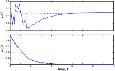
Figure 10: This figure shows a typical trajectory for a radiatively damped TLA undergoing homodyne-$x$ detection of efficiency $0.4$ (solid line). The dotted line represents the solution using our method whereas the dashed line represents the BG method. Both our method and the BG method were implemented using an ensemble size of 10000.

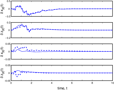
Figure 11: The top two plots show the difference between the exact solution and the BG method for $n=1000$ and 10000. The bottom two plots show the difference between the exact solution and our method for $n=1000$ and 10000.

In this paper we make two choices for $\Lambda(f_{2},r_{2},f_{1},r_{1})$. The first choice is $\Lambda(f_{2},r_{2},f_{1},r_{1})=\Lambda(f_{2})\Lambda(f_{1})\Lambda(r_{2})\Lambda(r_{1})$ where $\Lambda(r_{k})$ and $\Lambda(f_{k})$ are Gaussian distributions of variance $dt$ and mean $\lambda$ and $\mu$ respectively. The second choice is $\Lambda(f_{2},r_{2},f_{1},r_{1})=\Lambda(f_{2}|f_{1},r_{1})\Lambda(f_{1})\Lambda(r_{2})\Lambda(r_{1})$ where $\Lambda(r_{k})$ is the same as before but the fictitious results were chosen based on the true probability we would expect based on the past real and fictitious results up to but not including the current time. That is $\mu=\sqrt{\gamma_{2}}\,{\rm Tr[\hat{x}_{2}\bar{\rho}_{\bf R,F}(t)]}/{\rm Tr}[\bar{\rho}_{\bf R,F}(t)]$.

A third possible choice would be $\Lambda(f_{2},r_{2},f_{1},r_{1})=\Lambda(f_{2}|f_{1},r_{1})\Lambda(f_{1})\Lambda(r_{2}|r_{1},f_{1})\Lambda(r_{1})$, where both the real and fictitious distribution are chosen based on the past results up to but not including the current time. That is $\lambda=\sqrt{\gamma_{1}}\,{\rm Tr[\hat{x}_{1}\bar{\rho}_{\bf R,F}(t)]}/{\rm Tr}[\bar{\rho}_{\bf R,F}(t)]$ and $\mu=\sqrt{\gamma_{2}}\,{\rm Tr[\hat{x}_{2}\bar{\rho}_{\bf R,F}(t)]}/{\rm Tr}[\bar{\rho}_{\bf R,F}(t)]$. This would seem the closest choice to $P(f_{2},r_{2},f_{1},r_{1})$ but it is important to note that it is not the same. It is still an ostensible distribution, because the true distribution is based upon the entire measurement record, including results in the future. Thus our trajectory equations will still be unnormalized and we cannot replace $(r-\lambda)dt$ with $dW(t)$ as ${\rm Tr}[\hat{x}_{1}\bar{\rho}_{\bf R,F}(t)]/{\rm Tr}[\bar{\rho}_{\bf R,F}(t)]$ is not equal to ${\rm Tr[\hat{x}_{1}\rho_{\bf R}(t)]}$ for all possible fictitious records. If we were to make this substitution we would generate normalized equations, but averaging over all possible fictitious record would not give a typical trajectory for the state conditioned on the partial record ${\bf R}$. This is precisely the mistake Brun and Goan (BG) make in reference Brun .

To be more specific let us consider their approach and our approach for the following simple system: A two level atom radiatively damped and monitored using homodyne-$x$ detection with an efficiency $\eta$. That is this system is described by the SME

$$d\rho_{\bf R}(t)=dt\hat{\cal D}[\hat{\sigma}]\rho_{\bf R}+\sqrt{\eta}\,\hat{\cal H}[\hat{\sigma}]\rho_{\bf R}dW(t),$$ (131)

where $r(t+dt)dt=dW(t)+dt\sqrt{\eta}\,\langle\hat{\sigma}_{x}\rangle$. Now using BG’s theory we would extend this equation to

$$d\rho_{\bf R,F}(t) = dt\hat{\cal D}[\hat{\sigma}]\rho_{\bf R,F}+\sqrt{\eta}\,\hat{\cal H}[\hat{\sigma}]\rho_{\bf R,F}dW(t)$$ (132)

$$+\sqrt{1-\eta}\,\hat{\cal H}[\hat{\sigma}]\rho_{\bf R,F}d{\cal W}(t),$$

which has a pure state solution. Now they argue that by ensemble averaging over the fictitious noise process $d{\cal W}$ Eq. (131) is recovered. However this is incorrect. Although

$${\rm E}_{\cal W}[\sqrt{\eta}\,\hat{\cal H}[\hat{\sigma}]\rho_{\bf R,F}dW(t)]=\sqrt{\eta}\,{\rm E}_{\cal W}[\hat{\cal H}[\hat{\sigma}]\rho_{\bf R,F}]dW(t),$$ (133)

the nonlinearity in the superoperator $\hat{\cal H}$ means that

$${\rm E}_{\cal W}[\hat{\cal H}[\hat{\sigma}]\rho_{\bf R,F}]\neq\hat{\cal H}[\hat{\sigma}]{\rm E}_{\cal W}[\rho_{\bf R,F}]=\hat{\cal H}[\hat{\sigma}]\rho_{\bf R}.$$ (134)

To see this explicitly we expand Eq. (132) for two measurement (two steps in time)

$$\rho_{r_{1},r_{2},f_{1},f_{2}}(2dt)=$$

$$\hskip 28.45274pt\rho_{0}+dt\hat{\cal D}[\hat{\sigma}]\rho_{r_{1},f_{1}}+\sqrt{\eta}\,\hat{\cal H}[\hat{\sigma}]\rho_{r_{1},f_{1}}dW_{2}(t)+$$

$$\hskip 28.45274pt\sqrt{1-\eta}\,\hat{\cal H}[\hat{\sigma}]\rho_{r_{1},f_{1}}d{\cal W}_{2}(t)+dt\hat{\cal D}[\hat{\sigma}]\rho_{0}+$$

$$\hskip 28.45274pt\sqrt{\eta}\,\hat{\cal H}[\hat{\sigma}]\rho_{0}dW_{1}(t)+\sqrt{1-\eta}\,\hat{\cal H}[\hat{\sigma}]\rho_{0}d{\cal W}_{1}(t).\hskip 22.76228pt$$ (135)

Looking at this equation we see that the problem term is

$${\rm E}_{f_{1}}[\hat{\cal H}[\hat{\sigma}]\rho_{r_{1},f_{1}}] = {\rm E}_{f_{1}}[\hat{\sigma}\rho_{r_{1},f_{1}}+\rho_{r_{1},f_{1}}\hat{\sigma}$$ (136)

$$-{\rm Tr}[\hat{\sigma}_{x}\rho_{r_{1},f_{1}}]\rho_{r_{1},f_{1}}]$$

$$\neq \hat{\sigma}\rho_{r_{1}}+\rho_{r_{1}}\hat{\sigma}-{\rm Tr}[\hat{\sigma}_{x}\rho_{r_{1}}]\rho_{r_{1}}\hskip 22.76228pt$$

due to the non-linearity.

In our method this problem does not occur because we use ostensible distributions and linear equations. For this system the unnormalized state is

$$d\bar{\rho}_{\bf R,F}(t) = dt\hat{\cal D}[\hat{\sigma}]\bar{\rho}_{\bf R,F}+\sqrt{\eta}\,\bar{\cal H}_{\lambda}[\hat{\sigma}]\bar{\rho}_{\bf R,F}dt(r-\lambda)+$$ (137)

$$\sqrt{1-\eta}\,\bar{\cal H}_{\mu}[\hat{\sigma}]\bar{\rho}_{\bf R,F}d{\cal W}(t),$$

where $\bar{\cal H}_{\chi}[\hat{A}]\rho=\hat{A}\rho+\rho\hat{A}-\chi\rho$ with $\chi$ being either $\lambda$ or $\mu$. If we expand this to two measurements we find that the problem term does not occur as

$${\rm E}_{f_{1}}[\bar{\cal H}[\hat{\sigma}]\bar{\rho}_{r_{1},f_{1}}] = {\rm E}_{f_{1}}[\hat{\sigma}\bar{\rho}_{r_{1},f_{1}}+\bar{\rho}_{r_{1},f_{1}}\hat{\sigma}-\lambda\bar{\rho}_{r_{1},f_{1}}]$$ (138)

$$= \hat{\sigma}\rho_{r_{1}}+\rho_{r_{1}}\hat{\sigma}-\lambda\bar{\rho}_{r_{1}}.$$

To show the magnitude of the error in BG’s approach we numerically solved the SME for $\eta=0.4$ using Eq. (131), BG’s method and our method. We first randomly generate and store a string of $dW$’s, and use these to generate the true record ${\bf R}$ via Eq. (131). For BG’s method we use this string of $dW$’s, and generate an ensemble using randomly generate strings of $d{\cal W}$s. The resultant solution would, according to BG, correspond to the solution of Eq. (131). For our method, we use the true record ${\bf R}$ and again randomly generate strings of $d{\cal W}$s to obtain an ensemble average. The results of these simulations are shown in Figs. 10 and 11. Here we see that BG theory disagrees significantly with the exact result. Furthermore this discrepancy cannot be a statistical error as Fig. 11 shows that when the ensemble average is increased this difference remains approximately constant. That is, this simulation confirms that BG’s method fails to reproduce a typical solution to Eq. (131). By contrast our method reproduces Eq. (131) to within statistical error.

References

• (1) O. L. R. Jacobs, Introduction to Control Theory (Oxford University Press, Oxford 1993).
• (2) V. P. Belavkin, “Non-demolition measurement and control in quantum dynamical systems”, in Information, complexity, and control in quantum physics, edited by A. Blaquière, S. Dinar, and G.Lochak (Springer, New York, 1987) ; ibid, Commun. Math. Phys. 146, 611 (1992).
• (3) H. M. Wiseman and G. J.Milburn, Phys. Rev. Lett. 70, 548 (1993); ibid, Phys. Rev. A 49, 1350 (1994).
• (4) A. C. Doherty and K. Jacobs, Phys. Rev. A. 60, 2700 (1999); ibid, 62, 012105 (2000).
• (5) V. P. Belavkin and P. Staszewski, Phys. Rev. A 45, 1347 (1992).
• (6) H. J. Carmichael, An Open System Approach to Quantum Optics (Springer, Berlin,1993).
• (7) C. W. Gardiner, A. S. Parkins, and P.  Zoller, Phys. Rev. A 46, 4363 (1992).
• (8) K.  Mølmer, Y. Castin, and J. Dalibard, J. Opt. Soc. Am. B 10, 524 (1993).
• (9) H. M. Wiseman and G. Milburn, Phys. Rev. A 47,642 (1993).
• (10) P. Goetsch and R. Graham, Annal. der. Physik. 2, 706 (1993).
• (11) P. Goetsch and R. Graham, Phys. Rev. A 50, 5242 (1994).
• (12) H. M. Wiseman, Quantum Semiclass. Opt. 8, 205 (1996).
• (13) J. Gambetta and H. M. Wiseman, Phys. Rev. A 64, 042105 (2001).
• (14) H. M. Wiseman and L. Diósi, Chem. Phys. 268, 91 (2001).
• (15) C. W. Gardiner and P. Zoller, Quantum Noise (Springer, Berlin, 2000).
• (16) K. Kraus, States, Effects, and Operations: Fundamental Notions of Quantum Theory, vol. 190 of Lecture Notes in Physics (Springer, Berlin, 1983).
• (17) V. B. Braginsky and F. Y. Khalili, Quantum Measurement (University Press, Cambridge, 1992).
• (18) T. P. McGarty, Stochastic systems and state estimation (John Wiley & Sons, New York, 1974).
• (19) C. W. Gardiner, Handbook of Stochastic Methods: for Physics, Chemistry and the Natural Science (Springer, Berlin, 1985).
• (20) T. A. Brun and H. S. Goan, Phys. Rev. A 68, 032301 (2003).
• (21) P. Warszawski, H. M. Wiseman, and H. Mabuchi, Phys. Rev. A 65, 023802 (2001).
• (22) P. Warszawski and H. M. Wiseman, J. Opt. B: Quantum Semiclass. Opt. 5, 1 (2003); ibid 15 (2003).
• (23) P. Warszawski, J. Gambetta, and H. M. Wiseman, Phys. Rev. A 69, 042104 (2004).
• (24) N. P. Oxtoby, P. Warszawski, H. M. Wiseman, R. E. S.Polkinghorne, and H. B. Sun, Phys. Rev. B 71, 165317 (2005).
• (25) C. M. Caves, C. A. Fuchs, and R. Schack, J. Math. Phys. 43, 4537 (2002).
• (26) C. A. Fuchs, quant-ph/0205039.
• (27) G. Lindblad, Commun. Math. Phys. 48, 119 (1976).
• (28) D. Gatarek and N. Gisin, J. Math. Phys. 32, 2152 (1991).
• (29) G. E. P. Box and G. C. Tiao, Bayesian Inference in Statistical Analysis (Addison-Wesley, Sydney, 1973).