A Scheme of Generating and Spatially Separating Two-Component Entangled Atom Lasers

Abstract

Entanglement of remote atom lasers is obtained via quantum state transfer technique from lights to matter waves in a five-level $M$-type system. The considered atom-atom collisions can yield an effective Kerr susceptibility for this system and lead to the self- and cross- phase modulation between the two output atom lasers. This effect results in generation of entangled states of output fields. Particularly, under different conditions of space-dependent control fields, the entanglement of atom lasers and of atom-light fields can be obtained, respectively. Furthermore, based on the Bell-state measurement, an useful scheme is proposed to spatially separate the generated entangled atom lasers.

PACS numbers: 03.75.-b, 03.67.-a, 42.50.Gy

Quantum entanglement has always attracted great interest as it is one of the key differences between quantum and classical physics. Since it can be exploited for various novel applications such as quantum computation and precision measurements, there has been a continuing effort to engineer the robust quantum entangled states in different systems. Since the experimental realization of Bose-Einstein Condensation (BEC) in dilute atomic clouds in 1995, much efforts have been taken in preparing a continuous atom laser atom laser and exploring its potential applications in, e.g., gravity measurements through atom interferometry interferometer . The method for creating two correlated matter waves has been proposed via four-wave mixing using BECs several years ago deng , and the large amplification of the generated correlated matter waves was also achieved ketterle . Entanglement between the generated matter waves is possible when consider the coherent collisions between condensate atoms, which has been observed before coherence .

Here we propose a scheme to generate and spatially separate entangled atom lasers from a five-level $M$-type system, with coherent collisions between atoms considered. This technique is based on the physical mechanism of Electromagnetically Induced Transparency (EIT) 1 which has attracted much attention in both experimental and theoretical aspects 2 ; 3 ; 4 ; wu , especially for the rapid developments of quantum memory technique 5 , i.e., transferring the quantum states of photon wave-packet to collective Raman excitations in a loss-free and reversible manner. The quantum state transfer technique via EIT provides a new optical technique to generate continuous atom laser with extra quantum states 6 ; liu . Very recently, considering the nonlinear effect in the EIT quantum state transfer process, many intriguing applications were discovered by a series publications, such as the solitons formed by dark-state polaritons in the EIT Kerr medium 4 , generation of quantum phase gate for photons five and nonclassical soliton atom laser sal by considering the coherent atom-atom collisions.

In the following, firstly we investigate how to generate two-component entangled atom lasers by considering the atom-atom collisions in the quantum state transfer technique from lights to matter waves in a five-level $M$-type system. The considered atom-atom collisions can yield an effective Kerr susceptibility for the probe lights and lead to the self- and cross-phase modulation between the two output atom lasers. This effect is useful for generation of entangled states. Then, we propose a scheme to spatially separate the generated entangled atom lasers via entanglement swapping technique Bell .

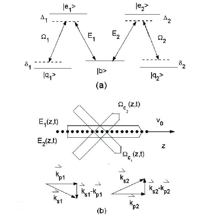
Figure 1: (a)Beam of $M$ type atoms coupled to two control fields and two quantized probe fields. (b)To minimize effect of Doppler-broadening, geometry is chosen such that $(\vec{k}_{pi}-\vec{k}_{si})\cdot\vec{e}_{z}\approx 0$ $(i=1,2)$.

The system we considered is shown in Fig.1. A beam of five-level $M$ type atoms moving in the $z$ direction interact with two quantized probe and two classical control Stokes fields 6 ; liu , and the former fields are taken to be much weaker than the later ones. Atoms in different internal states are described by five bosonic fields $\hat{\Psi}_{\mu}({\bf r},t)(\mu=b,q_{1},q_{2},e_{1},e_{2})$. The two Stokes fields coupling the transitions from the state $|q_{j}\rangle$ to excited one $|e_{j}\rangle$ $(j=1,2)$ can be described by the Rabi-frequencies $\Omega_{c_{j}}=\Omega_{0j}(z)e^{-i\omega_{s}(t-z/c_{j})}$, respectively, with $\Omega_{0j}$ being taken as real, and $c_{j}$ denoting the phase velocities projected onto the $z$ axis. The quantized probe fields coupling the transitions from the state $|b\rangle$ to $|e_{j}\rangle$ are characterized by the dimensionless positive frequency components $\hat{E}_{j}(z,t)=\hat{\cal E}_{j}(z,t)e^{-i\omega_{p_{j}}(t-z/c)}$. The Heisenberg equations for bosonic field operators under the $s$-wave approximation are governed by five

$$i\hbar\frac{\partial\hat{\Psi}_{b}}{\partial t} = [-\frac{\hbar^{2}}{2m}\nabla^{2}+\hbar\omega_{b}+V(\mathbb{r})+\mu_{b}\hat{\Psi}_{b}^{{\dagger}}\hat{\Psi}_{b}+\sum_{k=1,2}\mu_{bk}\hat{\Psi}_{q_{k}}^{{\dagger}}\hat{\Psi}_{q_{k}}]\hat{\Psi}_{b}$$ (1)

$$\ \ \ \ \ \ \ \ \ \ \ \ +\hbar g\hat{E}_{1}^{{\dagger}}\Psi_{e_{1}}+\hbar g\hat{E}_{2}^{{\dagger}}\hat{\Psi}_{e_{2}},$$

$$i\hbar\frac{\partial\hat{\Psi}_{q_{j}}}{\partial t} = [-\frac{\hbar^{2}}{2m}\nabla^{2}+\hbar\omega_{q_{j}}+V(\mathbb{r})]\hat{\Psi}_{q_{j}}+[\mu_{bj}\hat{\Psi}_{b}^{{\dagger}}\hat{\Psi}_{b}+\sum_{k=1,2}\mu_{jk}\hat{\Psi}_{q_{k}}^{{\dagger}}\hat{\Psi}_{q_{k}}]\hat{\Psi}_{q_{j}}$$ (2)

$$\ \ \ \ \ \ \ \ \ \ \ \ +\hbar\Omega_{c_{j}}^{*}\hat{\Psi}_{e_{j}},$$

$$i\hbar\frac{\partial\hat{\Psi}_{e_{j}}}{\partial t}=[-\frac{\hbar^{2}}{2m}\nabla^{2}+\hbar\omega_{e_{j}}+V(\mathbb{r})]\hat{\Psi}_{e_{j}}+\hbar\Omega_{c_{j}}\hat{\Psi}_{q_{j}}+\hbar g\hat{E}_{j}\hat{\Psi}_{b},$$ (3)

where $j=1,2$, $V(\mathbb{r})$ is the external trap potential, the scattering length $a_{ij}$ characterizes the atom-atom interactions via $\mu_{ij}=4\pi\hbar^{2}a_{ij}/m$ $i,j=b,1,2$ and $\omega_{j}$’s are the frequencies corresponding to the electronic energy levels. Since in present discussion almost no atoms occupy the excited states $|e_{1}\rangle$ or $|e_{2}\rangle$ in the dark-state condition that is fulfilled in EIT technique, the decay from the excited states and the collisions between the excited states and lower states can be safely neglected. The motion equations for the two quantized probe fields read

$$(\frac{\partial}{\partial t}+c\frac{\partial}{\partial z})\hat{E}_{1,2}(z,t)=ig\int d^{2}r_{\perp}\hat{\Psi}_{b}^{{\dagger}}\hat{\Psi}_{e_{1,2}}$$ (4)

where $r_{\perp}$ represents the transverse coordinate (perpendicular to the $z$ axis).

The transverse motion (perpendicular to the $z$ axis) of the beam is confined by the transverse trapping potential. Within the adiabatic condition the transverse motion can be restricted to the lowest transverse eigen-state adiabatic . For this the bosonic fields can be cast into two parts form , i.e. the transverse part and the longitudinal part (along $z$ axis). On the other hand, the EIT quantum state transfer process requires that the Rabi-frequencies of the Stocks control fields vary sufficiently slowly on the $z$ coordinate, and then all the bosonic fields’ amplitudes vary slowly with time and $z$ coordinate during the propagation, i.e., we can further conveniently introduce the slowly-varying amplitudes and a decomposition into velocity class 6 ; liu for the longitudinal part of each bosonic field. Therefore we rewrite the atomic fields as: $\hat{\Psi}_{b}=\sum_{l}\psi(\vec{r}_{\perp};z)\hat{\Phi}^{l}_{b}(z,t)e^{i(k_{l}z-\omega_{l}t)},\hat{\Psi}_{e_{j}}=\sum_{l}\psi(\vec{r}_{\perp};z)\hat{\Phi}^{l}_{e_{j}}(z,t)e^{i[(k_{l}+k_{p_{j}})z-(\omega_{l}+\omega_{p_{j}})t}$ and $\hat{\Psi}_{q_{j}}=\sum_{l}\psi(\vec{r}_{\perp};z)\hat{\Phi}^{l}_{q_{j}}(z,t)e^{i[(k_{l}+k_{p_{j}}-k_{s_{j}})z-(\omega_{l}+\omega_{p_{j}}-\omega_{c_{j}})t}$, where $j=1,2$, $\hbar\omega_{l}=\hbar^{2}k^{2}_{l}/2m$ is the corresponding kinetic energy in the $l$th velocity class, $k_{p_{j}}$ and $k_{s_{j}}$ $(j=1,2)$ are respectively the vector projections of the probe and Stokes fields to the $z$ axis. The atoms have a narrow velocity distribution around $v_{0}=\hbar{k_{0}}/m$ with $k_{0}\gg|k_{p}-k_{s}|$, and all fields are assumed to be in resonance for the central velocity class. $\hat{\Phi}^{l}_{\mu}(z,t)$ are the slowly-varying amplitudes that describe the motion of bosonic fields along $z$ axis, and $\psi(\vec{r}_{\perp};z)$ describes the equilibrium wave function (normalized to unity) in the transverse direction, i.e. $\int d^{2}r_{\perp}\psi^{*}(\vec{r}_{\perp};z)\psi(\vec{r}_{\perp};z)=1$. In our case the transverse trapping potential part $V(\vec{r}_{\perp})$ is set to be independent of $z$ and the effective longitudinal potential can then be taken to be zero (see ref. form ; Leboeuf ) (This requirement is similar to that in previous publications 6 ; liu ). Thus the equations of motion for the field operators can be recast into

$$\bigr{(}\frac{\partial}{\partial t}+\frac{\hbar k_{l}}{2m}\frac{\partial}{\partial z}\bigr{)}\Phi_{b}^{l}=-i\sum_{j=1,2}g\hat{\cal E}_{j}^{{\dagger}}\Phi^{l}_{e_{j}}-i\sum_{l}\bigr{(}\mu_{b}\Phi_{b}^{{\dagger}l}\Phi_{b}^{l}+\sum_{j=1,2}\mu_{bj}\Phi_{q_{j}}^{{\dagger}l}\Phi_{q_{j}}^{l}\bigr{)}\Phi_{b}^{l},$$ (5)

$$\bigr{(}\frac{\partial}{\partial t}+\frac{\hbar k_{l}}{2m}\frac{\partial}{\partial z}\bigr{)}\Phi_{q_{j}}^{l}=-i\delta_{j}^{l}\Phi_{q_{j}}^{l}-i\Omega_{0j}\Phi^{l}_{e_{j}}-i\sum_{k=1,2}\sum_{l}\bigr{(}\mu_{bk}\Phi_{b}^{{\dagger}l}\Phi_{b}^{l}+\mu_{jk}\Phi_{q_{k}}^{{\dagger}l}\Phi_{q_{k}}^{l}\bigr{)}\Phi_{q_{j}}^{l},$$ (6)

$$\bigr{(}\frac{\partial}{\partial t}+\frac{\hbar(k_{l}+k_{p_{j}})}{2m}\frac{\partial}{\partial z}\bigr{)}\Phi_{e_{j}}^{l}=-\Delta_{j}^{l}\Phi_{e_{j}}^{l}-ig\hat{\cal E}_{j}\Phi^{l}_{b}-i\Omega_{0j}\Phi^{l}_{q_{j}}.$$ (7)

and the two probe lights:

$$(\frac{\partial}{\partial t}+c\frac{\partial}{\partial z})\hat{\cal E}_{j}(z,t)=-ig\sum_{l}\hat{\Phi}_{b}^{{\dagger}l}\hat{\Phi}^{l}_{e_{j}},$$ (8)

where $\Delta^{l}_{j}\approx\hbar{k_{l}}k_{p_{j}}/m+(\omega_{e_{j}b}-\omega_{p_{j}})$ and $\delta^{l}_{j}\approx\hbar{k_{l}}(k_{p_{j}}-k_{s_{j}})/m+(\omega_{q_{j}b}-\omega_{p_{j}}-\omega_{c_{j}})$ are the single and two-photon detunings, respectively.

In order to solve the above equations of the matter-field operators, we shall consider the weak-probe-field approximation. In this case, consider a stationary input of atoms in state $|b\rangle$ and in zero order of the probe fields, the depletion of the atoms in the state $|b\rangle$ is neglected. Therefore we can make the replacement $\sum_{l}\Phi_{b}^{{\dagger}l}\Phi_{b}^{l}\rightarrow n$ 6 ; liu , where $n$ the constant total atomic density. Next, we shall consider the perfect one- and two-photon resonance case, i.e. $\Delta_{j}^{l}=0$ and $\delta_{j}^{l}+\mu_{bj}n=0$ so that we can apply an adiabatic approximation (the validity of this approximation will be discussed later) for the longitudinal motion of the fields and find: $\Phi^{l}_{e_{j}}=-\frac{1}{\Omega_{0j}}\sum_{k=1,2}\sum_{l}\mu_{jk}\Phi^{{\dagger}l}_{q_{k}}\Phi^{l}_{q_{k}}\Phi^{l}_{q_{j}}+\frac{i}{\Omega_{0j}}\bigr{(}\frac{\partial}{\partial t}+\frac{\hbar k_{l}}{2m}\frac{\partial}{\partial z}\bigr{)}\Phi^{l}_{q_{j}}$ and

$$\Phi^{l}_{q_{1}}\approx-\frac{g}{\Omega_{01}}\hat{\cal E}_{1}\Phi^{l}_{b},\ \ \ \Phi^{l}_{q_{2}}\approx-\frac{g}{\Omega_{02}}\hat{\cal E}_{2}\Phi^{l}_{b}$$

with $\Phi^{l}_{b}=\sqrt{n}\xi_{l}e^{-i(k_{l}z-\omega_{l}t)}$ and $\sum_{l}\xi_{l}=1$ 6 ; liu . Substitute these results into the above propagation equations of the two probe yields

$$\bigr{[}(1+\frac{g^{2}n}{\Omega^{2}_{0j}(z)})\frac{\partial}{\partial{t}}+c(1+\frac{g^{2}n}{\Omega^{2}_{0j}(z)}\frac{v_{0}}{c})\frac{\partial}{\partial{z}}\bigl{]}\hat{\cal E}_{j}(z,t)$$

$$+i\sum_{k=1,2}\frac{g^{4}n^{2}}{\Omega^{4}_{ok}(z)}\mu_{jk}\hat{\cal E}_{k}^{{\dagger}}\hat{\cal E}_{k}\hat{\cal E}_{j}(z,t)=\frac{g^{2}n}{\Omega^{2}_{0j}(z)}v_{0}(\frac{\partial}{\partial{z}}\ln\Omega_{0j}(z))\hat{\cal E}_{j}(z,t).$$ (9)

where $j=1,2$. The last part of the l.h.s of the this equation indicates an effective Kerr nonlinear interaction and the r.h.s. describes a reduction (enhancement) due to stimulated Raman adiabatic passage in two spatially varying Stokes fields for $v_{0}\neq 0$. With the definitions of the mixing angles $\theta_{j}$ by $\tan^{2}\theta(z)\equiv\frac{g^{2}n}{\Omega_{0}^{2}}\frac{v_{0}}{c}$, one finds the solutions for the probe fields:

$$\hat{\cal E}_{j}(z,t) = \exp\bigl{[}-i\sum_{k=1,2}\mu_{jk}\hat{\cal E}_{k}^{{\dagger}}(0,T_{j})\hat{\cal E}_{k}(0,T_{j})\int_{0}^{z}|\frac{\cos\theta_{j}(\xi)}{\cos\theta_{k}(0)}|^{2}\frac{g^{4}n^{2}}{\Omega^{2}_{0k}(\xi)(\Omega^{2}_{0j}(\xi)+g^{2}n\frac{v_{0}}{c})}d\xi\bigl{]}\times$$ (10)

$$\times\frac{\cos\theta_{j}(z)}{\cos\theta_{j}(0)}\hat{\cal E}_{j}\bigl{(}0,T_{j}\bigl{)},$$

where $T_{j}=t-\int dz^{\prime}/V^{j}_{g_{r}}$ with the group velocity $V^{j}_{g_{r}}=c(1+\frac{g^{2}n}{\Omega_{0j}^{2}}\frac{v_{0}}{c})/(1+\frac{g^{2}n}{\Omega_{0j}^{2}})$. The above formula clearly shows that the atom-atom collisions leads to self- and cross-phase modulation, and the additional phase is dependent on the Rabi-frequency $\Omega_{0}(z)$ of the stokes fields and the velocity $v_{0}$ of atomic beam. Assuming at the entrance point $\theta=0$, i.e. the both control fields are much stronger at the entrance point, one finds that the output two corresponding atom lasers read

$$\hat{\Phi}_{q_{1,2}}(z=L,t)=\sqrt{\frac{c}{v_{0}}}\exp\bigl{[}-i(\widehat{SPM}_{1,2}+\widehat{CPM}_{1,2})\bigl{]}\sin\theta_{1,2}(L)\hat{\cal E}_{1,2}(0,t),$$ (11)

where $\hat{\Phi}_{q_{j}}=\hat{\Psi}_{q_{j}}e^{-i[(k_{p_{j}}-k_{s_{j}})z-(\omega_{p_{j}}-\omega_{c_{j}})t]}$ and the self-phase-modulation $\widehat{SPM_{j}}$ and the cross-phase-modulation $\widehat{CPM_{j}}$ can easily be obtained from the eqs. (10)

$$\widehat{SPM_{j}}(z,t)=\mu_{jj}\hat{\cal E}_{j}^{{\dagger}}(0,T)\hat{\cal E}_{j}(0,T)\int_{0}^{z}\cos\theta_{j}^{2}(\xi)\sum_{k=1,2}\frac{(1-\Theta_{jk})g^{4}n^{2}}{\Omega^{2}_{0k}(\xi)(\Omega^{2}_{0j}(\xi)+g^{2}n\frac{v_{0}}{c})}d\xi,$$ (12)

$$\widehat{CPM_{j}}(z,t)=\sum_{j,k=1,2}\mu_{jk}(1-\Theta_{jk})\hat{\cal E}_{k}^{{\dagger}}(0,T)\hat{\cal E}_{k}(0,T)\int_{0}^{z}\cos\theta^{2}_{j}(\xi)\frac{g^{4}n^{2}}{\Omega^{2}_{0k}(\xi)(\Omega^{2}_{0j}(\xi)+g^{2}n\frac{v_{0}}{c})}d\xi,$$ (13)

where the symbol $\Theta_{jk}$ is defined by $\Theta_{jk}=1$ for $j=k$, and $\Theta_{jk}=1$ for $j\neq k$. The result (11) shows that when $\theta_{j}(L)=\pi/2$, i.e. the Rabi-frequency of control field $\Omega_{j}$ decreases to be much small at the output point, quantum states of probe light can be fully transferred to the corresponding output atomic laser.

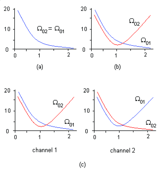
Figure 2: (color online) Space-dependent Rabi-frequencies of control fields. (a) the Rabi-frequencies $\Omega_{01}=\Omega_{02}$ so that $\theta_{1}(L)=\theta_{2}(L)=\pi/2$ at the output point. (b) $\theta_{1}(L)=\pi/2,\theta_{2}(L)=0$ at the output point. (c) For channel 1, $\theta_{1}(L)=\pi/2,\theta_{2}(L)=0$, whereas for channel 2, $\theta_{1}(L)=0,\theta_{2}(L)=\pi/2$.

The self-phase-modulation of the output states may lead to frequency-chirp effect and the cross-phase-modulation may lead to entanglement between the output states, which can be studied using proper space-varying control fields. Firstly, we consider the case shown in Fig.2(a), i.e. the mixing angles satisfy:

$$\theta_{1}(L)=\theta_{2}(L)=\pi/2.$$

In this case, the initial quantum states of probe lights are fully transferred to atom lasers associated with nontrivial phase shifts. For example, for the most “classical” states of two input probe lights $|\alpha\rangle\otimes|\beta\rangle$, where $|\alpha\rangle$ and $|\beta\rangle$ are single-mode coherent states, when $\mu_{11}=\mu_{22}=2\mu_{12}(=2\mu_{21})$, and the phase shift

$$\mu_{12}\int_{0}^{L}|\cos\theta_{j}(\xi)|^{2}\frac{g^{4}n^{2}}{\Omega^{2}_{0k}(\xi)(\Omega^{2}_{0j}(\xi)+g^{2}n\frac{v_{0}}{c})}d\xi=\pi,$$ (14)

with $j=1$ for $k=2$ and $j=2$ for $k=1$, the output state of the two atom lasers can be verified as $|\Psi\rangle_{atom}=\frac{1}{2}(|\bar{\alpha},\bar{\beta}\rangle+|-\bar{\alpha},\bar{\beta}\rangle+|\bar{\alpha},-\bar{\beta}\rangle-|-\bar{\alpha},-\bar{\beta}\rangle)$ with $\bar{\alpha}=\sqrt{c/v_{0}}\alpha,\bar{\beta}=\sqrt{c/v_{0}}\beta$. This is an entangled superposition of macroscopically distinguishable states. Furthermore, if we consider the case shown in Fig.2(b), i.e. the mixing angle $\theta_{1}(L)=\pi/2$ whereas $\theta_{2}(L)=0$, only the atom laser $\hat{\Phi}_{q_{1}}$ is generated and the second probe light is emitted out. In this way, under the condition of Eq. (14), we find the input state $|\alpha\rangle\otimes|\beta\rangle$ finally evolves into

$$|\Psi\rangle_{a-l}=\frac{1}{2}|\bar{\alpha}\rangle_{A}\bigr{(}|\beta\rangle+|-\beta\rangle\bigr{)}_{L}+\frac{1}{2}|-\bar{\alpha}\rangle_{A}\bigr{(}|\beta\rangle-|-\beta\rangle\bigr{)}_{L},$$ (15)

where $A$, $L$ represent the output $atom$ $laser$ and $probe$ $light$, respectively. Eq. (15) shows that the entangled state between atom laser and photons can be readily obtained with our model. Since light speed is much larger than that of the generated atom laser, the above entanglement is between two distant qubits. This result is useful for quantum teleportation.

However, a challenge is still left for the two entangled atom lasers: Since they propagate in the same direction, generally the entanglement of the output atom lasers $|\Psi\rangle_{atom}$ is local, whereas for practical applications we should separate them spatially. This issue can be studied with entanglement swapping technique Bell ; Bell2 .

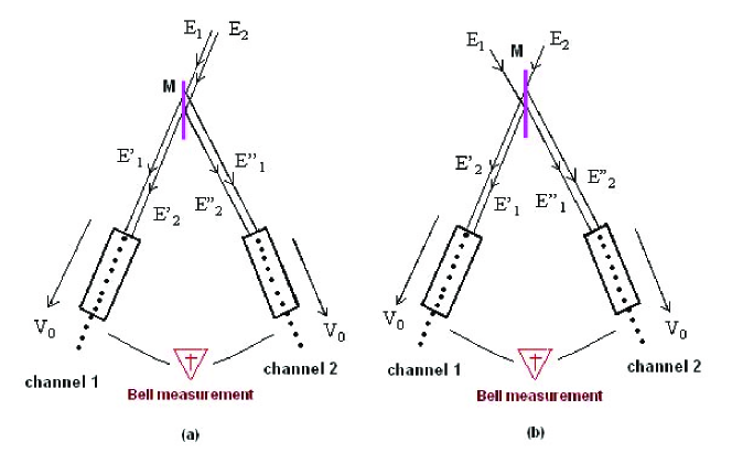
Figure 3: (color online) (a)(b) The schematic set-up for generation of two spatially separated entangled atom lasers under the condition shown in Fig. 2(c). Based on the Bell measurement on the photon states, the output atom lasers become entangled.

The schematic set-up is shown in Fig. 3, by which we demonstrate how to spatially separate the two-component entangled atom lasers. M is a semitransparent mirror splitter, through which the two input probe pulses $\hat{E}_{1}(z,t)$ and $\hat{E}_{2}(z^{\prime},t)$ are split into four pulses with identical expectative intensities, i.e. $\hat{E}^{\prime}_{1}(z,t)$, $\hat{E}^{\prime}_{2}(z,t)$, $\hat{E}^{\prime\prime}_{1}(z^{\prime}t)$ and $\hat{E}^{\prime\prime}_{2}(z^{\prime},t)$ with their amplitudes equal each other. After these splitters, the four pulses enter the two channels (channel 1 and channel 2), respectively. Also consider the input coherent states of two probe lights $|\alpha\rangle\otimes|\beta\rangle$, together with the conditions shown in Fig. 2(c) and eq. (14), we find the output states from the two channels

$$|\Psi\rangle = |\Psi\rangle_{1}\otimes|\Psi\rangle_{2}$$

$$= \frac{1}{4}\bigl{(}|\frac{\bar{\alpha}}{\sqrt{2}}\rangle_{1A}\otimes(|\frac{\beta}{\sqrt{2}}\rangle+|\frac{-\beta}{\sqrt{2}}\rangle)_{1L}+|\frac{-\bar{\alpha}}{\sqrt{2}}\rangle_{1A}\otimes(|\frac{\beta}{\sqrt{2}}\rangle-|\frac{-\beta}{\sqrt{2}}\rangle)_{1L}\bigl{)}\otimes$$

$$\otimes\bigl{(}|\frac{\alpha}{\sqrt{2}}\rangle_{2L}\otimes(|\frac{\bar{\beta}}{\sqrt{2}}\rangle+|\frac{-\bar{\beta}}{\sqrt{2}}\rangle)_{2A}+|\frac{-\alpha}{\sqrt{2}}\rangle_{2L}\otimes(|\frac{\bar{\beta}}{\sqrt{2}}\rangle-|\frac{-\bar{\beta}}{\sqrt{2}}\rangle)_{2A}\bigl{)}$$

$$= \frac{1}{4}\bigl{(}\sqrt{N_{+}N^{\prime}_{+}}|\frac{\bar{\alpha}}{\sqrt{2}}\rangle_{1A}\otimes|\frac{\bar{\beta}}{\sqrt{2}}\rangle_{2A}\otimes|+\rangle_{1L}\otimes|+\rangle_{2L}+\sqrt{N_{+}N^{\prime}_{-}}|\frac{\bar{\alpha}}{\sqrt{2}}\rangle_{1A}\otimes|\frac{-\bar{\beta}}{\sqrt{2}}\rangle_{2A}\otimes|+\rangle_{1L}\otimes|-\rangle_{2L}$$

$$+\sqrt{N^{\prime}_{+}N_{-}}|\frac{-\bar{\alpha}}{\sqrt{2}}\rangle_{1A}\otimes|\frac{\bar{\beta}}{\sqrt{2}}\rangle_{2A}\otimes|-\rangle_{1L}\otimes|+\rangle_{2L}+\sqrt{N_{-}N^{\prime}_{-}}|\frac{-\bar{\alpha}}{\sqrt{2}}\rangle_{1A}\otimes|\frac{-\bar{\beta}}{\sqrt{2}}\rangle_{2A}\otimes|-\rangle_{1L}\otimes|-\rangle_{2L}\bigl{)},$$

where $|\Psi\rangle_{1}$ and $|\Psi\rangle_{2}$ represent the output states from channel 1 and channel 2. The orthogonal bases are defined as $|\pm\rangle_{1L}=\frac{1}{\sqrt{N_{\pm}}}\bigl{(}|\frac{\beta}{\sqrt{2}}\rangle_{1L}\pm|\frac{-\beta}{\sqrt{2}}\rangle_{1L}\bigl{)}$ and $|\pm\rangle_{2L}=\frac{1}{\sqrt{N^{\prime}_{\pm}}}\bigl{(}|\frac{\alpha}{\sqrt{2}}\rangle_{2L}\pm|\frac{-\alpha}{\sqrt{2}}\rangle_{2L}\bigl{)}$ which correspond to quantum states of light fields output from channel $1$ and channel $2$, respectively, with the normalized factors $N_{\pm}=2\pm 2e^{-|\alpha|^{2}}$ and $N^{\prime}_{\pm}=2\pm 2e^{-|\beta|^{2}}$. The factorizable state in eq.(A Scheme of Generating and Spatially Separating Two-Component Entangled Atom Lasers) can be transferred to an entangled one via Bell-state measurement on the orthogonal photon states $|\pm\rangle$. For this we define the Bell bases as $\psi^{\pm}=\frac{1}{2}\bigr{(}|+\rangle_{1L}|-\rangle_{2L}\pm|-\rangle_{1L}|+\rangle_{2L}\bigr{)}$ and $\phi^{\pm}=\frac{1}{2}\bigr{(}|+\rangle_{1L}|+\rangle_{2L}\pm|-\rangle_{1L}|-\rangle_{2L}\bigr{)}$. Using Bell-state measurements the eq. (A Scheme of Generating and Spatially Separating Two-Component Entangled Atom Lasers) can be recast into the following entangled states

$$|\Psi\rangle^{\pm}_{12A}=\frac{1}{2}\sqrt{N_{+}N^{\prime}_{-}}|\frac{\bar{\alpha}}{\sqrt{2}}\rangle_{1}\otimes|\frac{-\bar{\beta}}{\sqrt{2}}\rangle_{2}\pm\frac{1}{2}\sqrt{N^{\prime}_{+}N_{-}}|\frac{-\bar{\alpha}}{\sqrt{2}}\rangle_{1}\otimes|\frac{\bar{\beta}}{\sqrt{2}}\rangle_{2},$$ (17)

and

$$|\Phi\rangle^{\pm}_{12A}=\frac{1}{2}\sqrt{N_{+}N^{\prime}_{+}}|\frac{\bar{\alpha}}{\sqrt{2}}\rangle_{1}\otimes|\frac{\bar{\beta}}{\sqrt{2}}\rangle_{2}\pm\frac{1}{2}\sqrt{N^{\prime}_{-}N_{-}}|\frac{-\bar{\alpha}}{\sqrt{2}}\rangle_{1}\otimes|\frac{-\bar{\beta}}{\sqrt{2}}\rangle_{2},$$ (18)

respectively. The above results also show that the entanglement of final states can be controlled with present EIT technique and proper Bell-state measurements. Particularly, when $\alpha=\beta$, the state $|\Psi\rangle^{-}_{12A}$ reduces into the maximum entangled state. By now we successfully generate entangled states of two-component spatially separated atom lasers, for which the Schrodinger cat state is not needed for the input probe lights. Noting that the Bell measurements on the photon states has been widely studied Bell2 , the present scheme of spatially separating the entangled atom lasers will be interesting for quantum information processing.

Before conclusion, we would like to emphasize validity of the approximations used in above derivation. Firstly, for the adiabatic condition we have assumed the perfect two-photon resonance and zero decay from the excited states. The non-vanishing two-photon detunings can lead to an additional term in the expansion of field $\Phi^{l}_{e_{j}}$:

$$\hat{\Phi}^{l}_{e_{j}}\rightarrow\hat{\Phi}^{l}_{e_{j}}+\frac{\Omega^{2}_{0j}(\delta_{j}+\mu_{jb}n)}{\Omega^{2}_{0j}-(\delta_{j}+\mu_{jb}n)(\Delta-i\gamma)}\frac{g\hat{\cal E}_{j}}{\Omega_{0j}}\hat{\Phi}^{l}_{b},\ \ j=1,2,$$ (19)

where the decay rate $\gamma$ from the excited states are considered. Apparently the imaginary part in above formula can lead to a loss in the solution of equation of probe fields: ${\cal E}_{j}(z,t)\rightarrow e^{-\eta_{j}}{\cal E}_{j}(z,t)$ with $\eta_{j}>0$. Here the calculation of factor $\eta_{j}$ is the same with that in ref. 6 and one can easily obtain $\eta_{j}\leq|\delta_{j}+\mu_{jb}n|L/v_{0}$. Thus when $\eta_{j}\leq|\delta_{j}+\mu_{jb}n|\frac{L}{v_{0}}\ll 1$, the loss can be safely neglected. As we know the residual Doppler shift of the $|q_{j}\rangle\rightarrow|e_{j}\rangle$ transition can result in a two-photon detuning through $\delta_{j}=\Delta v(\vec{k}_{pj}-\vec{k}_{sj})\cdot\vec{e}_{z}(j=1,2)$, where $\Delta{v}$ denotes the difference of the velocity in $z$ direction with respect to the resonant velocity class, present condition also reads $\Delta v/v_{0}\ll\min\{\frac{1}{|k_{p_{j}}-k_{s_{j}}|}(\frac{1}{L}-\frac{\mu_{bj}n}{v_{0}}),j=1,2\}$ and $\frac{v_{0}}{\mu_{bj}nL}>1$. The later condition is easy to satisfied, because $\mu_{bj}n=4\pi n\hbar^{2}a_{bj}/m\ (a_{bj}\sim nm)$ is a much small factor. Another limitation of the above discussion is set by the dephasing of the atom fields during their propagation time $\Delta T$ from the entrance to the output point. Obviously, $\Delta T$ can be chosen as small as (generally larger than) the initial pulse length, and the compressed length in the medium $\Delta L=V_{g_{r}}\Delta T$ should still sufficiently larger than the wave length $\lambda$. Since the group velocity is larger (or equal) than the propagation velocity $v_{0}$ of the atomic beam ($V_{g_{r}}\rightarrow v_{0}$, when $\Omega_{0}\rightarrow 0$), the condition $\Delta L\gg\lambda$ can easily be satisfied.

In conclusion we obtain two-component spatially separated entangled atom lasers via quantum state transfer technique in a five-level $M$-type system. The atom-atom collisions can yield an effective Kerr susceptibility for this system and lead to the self- and cross-phase modulation between the output atom/light fields. This effect results in a large phase shift, which is dependent on the factor $c/v_{0}$ and the space distribution of Rabi-frequency $\Omega_{0j}(z)$ of the stokes fields, for the output fields and has potential applications. Particularly, considering the most “classical”, non-entangled coherent input lights and under different conditions of space-dependent control fields, we can obtain the entanglement of atom lasers and of atom-light fields, etc. Furthermore, based on the Bell-state measurement, an useful scheme is proposed to spatially separate the generated entangled atom lasers in our paper. Under proper Bell-state measurement, one can even obtain the maximum entanglement of remote atom lasers. The large phase shift can also be used to implement a quantum phase gate between two dark-state polaritons (DSPs) 5 ; 6 ; liu (whose input states are photons and output states are atom lasers) when the input quantized probe lights are both in the single-photon state.

This work is supported by NSF of China under grants No.10275036 and No.10304020, and by NUS academic research Grant No. WBS: R-144-000-071-305.

References

• (1) M.-O. Mewes et al., Phys.Rev.Lett., 78,582(1997); M. R. Andrews et al., Science 275,637(1997).
• (2) J. Baudon et al., J. Phys. B: At. Mol. Opt. Phys. 32, R173 (1999); A. Peters et al., Metrologia 38, 25 (2001); Y. Shin et al., Phys. Rev. Lett. 92,050405(2004).
• (3) L. Deng et al., Nature (London) 398, 218 (1999).
• (4) J. M. Vogels, K. Xu and W. Ketterle, Phys. Rev. Lett. 89, 020401(2002).
• (5) M. Greiner et al., Nature (Lodon) 419, 21 (2002); F. Dalfovo et al., Rev. Mod. Phys. 71, 463 (1999).
• (6) S. E. Harris, J. E. Field and A. Kasapi, Phys. Rev. A 46, R29 (1992); M. O. Scully and M. S. Zubairy, Quantum Optics (Cambridge University Press, Cambridge 1999).
• (7) L.V.Hau et al., Nature (London) 397, 594(1999); C. Liu et al., Nature (London) 409, 490(2001); D. F. Phillips et al., Phys. Rev. Lett. 86,783(2001);
• (8) L. Deng et al., Phys. Rev. A 64, 023807 (2001); L. Deng et al., Phys. Rev. A 64, 031802 (2001); L. Deng et al., Phys. Rev. A 65, 051805 (2002); M. Kozuma et al., Phys. Rev. A 66, 031801 (2002) M. D. Lukin et al., Phys. Rev. Lett. 84, 4232(2000).
• (9) X. J. Liu, H. Jing and M. L. Ge, Phys. Rev. A, 70, 055802 (2004).
• (10) Y. Wu and L. Deng, Phys. Rev. Lett. 93, 143904 (2004); Y. Wu and L. Deng, Opt. Lett. 29, 2064-2066 (2004); Y. Wu and X. Yang, Phys. Rev. A 70, 053818 (2004); Y. Wu, Phys. Rev. A, 71, 053820 (2005)..
• (11) M. Fleischhauer et al., Phys. Rev. Lett. 84, 5094 (2000); M.Fleischhauer et al., Phys. Rev. A 65,022314 (2002); C. P. Sun, Y. Li, and X. F. Liu, Phys. Rev. Lett. 91,147903 (2003).
• (12) M. Fleischhauer and S. Q. Gong, Phys. Rev. Lett. 88, 070404 (2002).
• (13) Xiong-Jun Liu, Hui Jing, Xiao-Ting Zhou, and Mo-Lin Ge Phys. Rev. A 70, 015603(2004).
• (14) M. MaΕ‘alas and M. Fleischhauer., Phys. Rev. A, 69, 061801(RC)(2004).
• (15) Xiong-Jun Liu, Hui Jing and Mo-Lin Ge, e-print: arXiv:quant-ph/0406043(2004).
• (16) M. Zukowski et al., Phys. Rev. Lett. 71, 4287 (1993); J. W. Pan et al., ibid. 80, 3891(1998); Xiaoguang Wang et al., Phys. Rev. A 65,012303(2001).
• (17) A. Kitagawa and K. Yamamoto, Phys. Rev. A 70, 052311 (2004); L. MiΕ‘ta, Jr. and R. Filip, Phys. Rev. A 71, 032342 (2005).
• (18) L. I. Glazman et al., JETP Lett. 48, 238 (1998).
• (19) A. D. Jackson et al., Phys. Rev. A 58, 2417 (1998).
• (20) P. Leboeuf, N. Pavloff and S. Sinha, Phys. Rev. A 68, 063608 (2003).
• (21) M. D. Lukin et al., Phys. Rev. Lett. 84, 1419 (2000); M. Paternostro et al., Phys. Rev. A 67, 023811 (2003).
Refer to caption