Gravitational field measurement with an equilibrium ensemble of cold atoms

Abstract

A new approach to the measurement of gravitational fields with an equilibrium ensemble of ultra-cold alkali atoms confined in a cell of volume $V$ is investigated. The proposed model of the gravitational sensor is based on a variation of the density profile of the ensemble due to changing of the gravitational field. For measurement the atomic density variations of the ensemble the electromagnetically induced transparency method is used.
PACS number(s): 39.20.+q, 03.75.Dg, 04.80.-y, 32.80.Pj, 42.50.Gy

Gravitational sensors operating on technologies of atom optics usually use a variety of atom interferometry techniques for the detection of gradient of the gravitational potential cla -pet . Atom interferometry requires elements equivalent to beam splitters and mirrors of light interferometry ai -mey . These elements complicate the gravitational sensor’s design and impose limitations on its sensitivity. The objective of this work is to provide a scheme of gravitational sensor excluding atom interferometry technique. We will investigate the posibility of gravitational field measurement with an equilibrium ensemble of ultra-cold alkali atoms (medium) confined in a cell of a volume $V$. The density profile of this medium is changed due to the interaction of its atoms with the gravitational field. The gravitational field can be measured by measuring the phase shift of an optical beam passing through the medium. For measuring the density variation of the medium, the electromagnetically induced transparency technique is used bol -har2 . The sensitivity of the idialized model of the proposed gravitational sensor is comparable with the sensitivity of modern atom interferometric gravimeter.

Let us consider an atomic cloud confined and cooled inside a thin-walled cell of a small volume $V$. The technique of alkali atom cooling is well developed and presented in a number of publications wie -har . After the trapping potential is turned off the cloud will expand filling all volume $V$. We will consider that on this stage the atomic ensemble is only under the influence of a gravitational field and will neglect the heat exchange between the ensemble of alkali atoms and the cell during the measurement time. The field theoretical Hamiltonian of the ensemble in the presence of the external gravitational field is written as

$$\hat{H}=\int d^{3}\vec{x}\psi^{+}(\vec{x},t)\left[-\frac{\hbar^{2}}{2m}\nabla^{2}+V(\vec{x})\right]\psi(\vec{x},t)$$

$$+\frac{1}{2}\int d^{3}\vec{x}^{\prime}d^{3}\vec{x}\psi^{+}(\vec{x},t)\psi^{+}(\vec{x}^{\prime},t)U(\vec{x},\vec{x}^{\prime})\psi(\vec{x},t)\psi(\vec{x}^{\prime},t),$$ (1)

where $\psi(\vec{x},t)$ and $\psi^{+}(\vec{x},t)$ are field operators, $V(\vec{x})$ is the atom-gravitational field interaction potential, $m$ is the atomic mass, and $U(\vec{x},\vec{x}^{\prime})$ is the two body interatomic potential dalf . Operator $\psi(\vec{x},t)$ creates an atom at the point $\vec{x}$ and time $t$ while $\psi^{+}(\vec{x},t)$ annihilates an atom. The field operators obey the following commutation relations: $[\psi(\vec{x},t),\psi(\vec{x}^{\prime},t)]=0$ and $[\psi(\vec{x},t),\psi^{+}(\vec{x}^{\prime},t)]=\delta^{3}(\vec{x}-\vec{x}^{\prime})$, which define the statistics of the ensemble. We can also introduce a number operator

$$\hat{N}=\int d^{3}\vec{x}\psi^{+}(\vec{x},t)\psi(\vec{x},t)$$ (2)

with the eigenvalues interpreted as the number of the atoms. For further analysis we will use the grand partition function of the atomic medium

$$Z={\rm Sp}\left[\exp{(\beta(\mu\hat{N}-\hat{H}))}\right],$$ (3)

where $\mu$ is the chemical potential, and $\beta=1/k_{B}T$ is the inverse temperature ($k_{B}$ is the Boltzmann constant). If atoms of the medium are under the influence of only a gravitational field, then the potential of interaction is given by the classical equation $V(\vec{x})=m\Phi(\vec{x})$, where $\Phi(\vec{x})$ is the Newtonian gravitational potential. Inserting (1) and (2) into (3) and neglecting interatomic interactions grav we obtain the grand partition function in the form

$$Z=\prod_{i}\left[1-\exp{(-\beta(\epsilon_{i}-\mu))}\right]^{-1},$$ (4)

where $\epsilon_{i}$ is the energy of a boson in $i$-th state. Statistical and thermodynamical properties of the medium can be investigated with the help of a grand thermodynamic potential given by $\Omega=-(1/\beta)\ln Z$. Using the equation (4) we obtain the expression for the thermodynamic potential in the form

$$\Omega=(1/\beta)\sum_{i}\ln\left[1-\exp{(-\beta(\epsilon_{i}-\mu))}\right].$$ (5)

In quasi-classical regime we can replace in the equation (5) the summation over single atomic states by the integration $\sum\nolimits_{i}\rightarrow s\int(2\pi\hbar)^{-3}d\Gamma$ , where $d\Gamma=d^{3}\vec{p}d^{3}\vec{x}$, and $s$ is the number of the possible spin states of the atom. The atomic energy in this case can be represented by a sum of kinetic and potential energies $\epsilon_{i}={\vec{p}~{}}^{2}/2m+m\Phi(\vec{x})$ and the expression for the grand thermodynamic potential will be

$$\Omega=(1/\beta)\int\frac{sd\Gamma}{(2\pi\hbar)^{3}}\ln\left[1-z(\Phi)\exp{(-\beta p^{2}/2m)}\right],$$ (6)

where the gravity dependent fugacity $z$ is given by the equation

$$z(\Phi)=\exp\left[\beta(\mu-m\Phi)\right].$$ (7)

The grand thermodynamic potential (6) can be written in the form $\Omega=\int d^{3}\vec{x}\omega(\vec{x})$ where the density of grand thermodynamic potential is given by the equation

$$\omega=(1/\beta)\int\frac{sd^{3}\vec{p}}{(2\pi\hbar)^{3}}\ln\left[1-z(\Phi)\exp{(-\beta p^{2}/2m)}\right].$$ (8)

The average density of atoms in the medium is found as $N=-(\partial\omega/\partial\mu)$ and has the following form

$$N=\int\frac{d^{3}\vec{p}}{(2\pi\hbar)^{3}}\frac{s}{z^{-1}(\Phi)\exp(\beta p^{2}/2m))-1}.$$ (9)

The integration of (9) yields

$$N\lambda^{3}_{dB}=g_{3/2}(z),$$ (10)

where $\lambda_{dB}=\sqrt{2\pi\hbar^{2}\beta/m}$ is the thermal de Broglie wavelength and $g_{3/2}(z)$ is a function defined by the equation

$$g_{k}(z)=\sum^{\infty}_{n=1}\frac{z^{n}}{n^{k}}.$$ (11)

The functions $g_{k}(z)$ obey the recursion relations

$$z\frac{d}{dz}g_{k}(z)=g_{k-1}(z)$$ (12)

and have the following integral representations

$$g_{k}(z)=\frac{2^{2k-1}}{\sqrt{\pi}}\frac{\Gamma(k-1/2)}{\Gamma(2k-1)}\int^{\infty}_{0}dx\frac{x^{2k-1}}{z^{-1}\exp(x^{2})-1},$$ (13)

where $\Gamma(k)$ is the gamma function. The functions $g_{k}(z)$ have singularity at $z=1$ , which leads to BEC, moreover, the series (11) converges only for $k>1$. The equation (10) describes the relation between the density of particles $N$, temperature $T$ and the gravity dependent fugacity $z$. The variation of the atomic density of the medium is found from (10) in the form

$$\delta N=-\beta mN_{0}F(z_{0})\delta\Phi,$$ (14)

where $F(z)$ is given by the equation $F(z)=g_{1/2}(z)/g_{3/2}(z)$. In the equation (14) the atomic density variation $\delta N=N-N_{0}$, and the variation of gravitational potential $\delta\Phi=\Phi(\vec{x})-\Phi({\vec{x}}_{0})$ are defined between points $\vec{x}$ and ${\vec{x}}_{0}$. Fugacity $z_{0}$ at point ${\vec{x}}_{0}$ is related to $N_{0}$ and temperature $T$ of the medium by the equation (10). Let us select the coordinate system $\{x^{1},x^{2},x^{3}\}$, where the vector of gravitational acceleration is $\vec{g}=\{0,0,-g\}$. In this coordinate system the variation of gravitational potential can be written as $\delta\Phi=gY$, where $Y=(x^{3}-x^{3}_{0})$ is the displacement between two points along $x^{3}$-axis.

The equation (14) can be used for the analysis of the influence of gravitational field on the medium consisting of non-interacting alkali atoms in the cell of volume $V$. Let us rewrite it in the form

$$\delta N=-N_{0}\beta mYF(z_{0})g.$$ (15)

As follows from this equation, the gradient of gravitational potential causes the variation of the atomic density of the medium in the cell that can be detected with electromagnetically induced transparency (EIT) technique in the combination with the method of optical interferometry (Fig. 1).

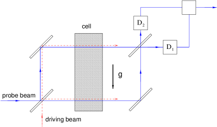
Figure 1: Mach-Zehnder interferometer detects the phase shift of the probe beams after they pass through the cooled atomic medium placed in the cell of the volume $V=1~{}cm^{3}$. The gradient of gravitational potential causing the phase shift is given by an arrow. The cell has the length $L$, and the upper and the lower beams of the interferometer are separated by the distance $Y$. Dashed arrows correspond to driving fields.

Let us consider EIT effect in application to the medium in gravitational field by taking into account the internal structure of bosons. We will assume that each boson of the medium is a three-level system with one upper (a) and two lower levels (b) and (c). To obtain EIT conditions, two optical (driving and probe) fields are used. Let the driving field of Rabi frequency $\Omega$ couple the levels (a-c) whereas the probe field of frequency $\omega$ couple the levels (a-b). The driving field provides an interference of different possible absorption pathways producing no absorption effect har3 . As the result, the medium becomes transparent to a probe field and the real part of susceptibility $\chi^{\prime}$ of the probe frequency near the resonant point will be

$$\chi^{\prime}=-\frac{\wp^{2}}{\hbar\varepsilon_{0}}\frac{\Delta}{\Omega^{2}}N,$$ (16)

where $\wp$ is the $a\rightarrow b$ transition matrix element, $N$ is the atomic density, and $\Delta_{ab}=\omega_{ab}-\omega$ is the atom-probe field detuning sc . The dispersive properties of the medium are defined by refractive index $n=1+\chi^{\prime}/2$, which is written in the form

$$n=1-\frac{\wp^{2}}{2\hbar\varepsilon_{0}}\frac{\Delta}{\Omega^{2}}N.$$ (17)

As follows from Fig.1, the interferometric phase shift $\phi$ of probe beams is a function of the variation of refractive index $\delta n$ of the medium

$$\phi=\frac{2\pi L}{\lambda}\delta n,$$ (18)

where $\lambda$ is the wavelength of the probe field, and $L$ is the length of the cell. Interaction of atoms of the medium with gravitational field changes the density profile of the medium. The density variation in the medium leads to variation of the refractive index along the gradient of gravitational field. When two separated probe beams pass the medium at points of different gravitational potential, they gain the phase shift depending on the gradient of the gravitational potential. Therefore the gradient of the gravitational potential can be measured by measuring the phase shift of probe beams in the interferometer.

From the equations (15), (17) and (18) we obtain the relation between the phase shift and the gravitational acceleration. The variation of the refractive index is found from the equation (17) as

$$\delta n=\left[\frac{3}{8\pi^{2}}\frac{\lambda^{3}\gamma\Delta}{\Omega^{2}}\right]\delta N,$$ (19)

where $\gamma=\wp^{2}\omega^{3}/(6\pi\hbar\varepsilon_{0}c^{3})$ is the radiative decay from the upper level. Then the phase shift of the two beams in the interferometer will be

$$\phi=\left[\frac{3}{4\pi}\frac{L\lambda^{2}\gamma\Delta}{\Omega^{2}}\right]\delta N.$$ (20)

Inserting the equation (15) into the equation (20) we get

$$\phi=\left[\frac{3}{4\pi}\frac{A\lambda^{2}\gamma^{2}xN_{0}mF(z_{0})}{k_{B}T\Omega^{2}}\right]g,$$ (21)

where $A=LY$ is the area of the side surface of the medium, and $x=\Delta/\gamma$ is the dimensionless detuning scale. The limiting sensitivity of the device is defined by the equation

$$\delta g=\left[\frac{3}{4\pi}\frac{A\lambda^{2}\gamma^{2}xN_{0}mF(z_{0})}{k_{B}T\Omega^{2}}\right]^{-1}\delta\phi.$$ (22)

For numerical demonstration of the limiting sensitivity of this gravitational sensor, we will assume that the driving field is strong and $\Omega\approx\gamma$ fsc . Taking into account that $F(z)\geq 1$, and putting for simplicity $xF(z)\approx 1$ we can rewrite the equation (22) in a simple form ik

$$\delta g=\left[\frac{4\pi}{3}\frac{k_{B}}{A\lambda^{2}N_{0}m}\right]T\delta\phi.$$ (23)

For a wavelength $\lambda=500~{}{\rm nm}$, atomic density $N_{0}=10^{12}~{}{\rm cm^{-3}}$, atomic mass $m=10^{-26}~{}{\rm kg}$, and the side area of the cell $A=1~{}{\rm cm^{2}}$, we find that the coefficient of the equation (23) in square bracket is of the order of ten and, therefore, one can simplify the equation (23) as $\delta g\approx 10T\delta\phi$. Assuming the temperature of the gas is about $T=1~{}{m\rm K}$ and computing the sensitivity of the interferometer with the equation $\delta\phi=\sqrt{\hbar\omega/P_{p}\tau}$ for $P_{p}=1~{}m$W probe beam power and $\tau=1$ second of measurement time, we find that the minimal detectable gravitational field changing is $\delta g\approx 10^{-11}~{}{\rm g}$. As follows from the equation (23), the important factor contributing to the sensitivity of the sensor is the side area of the cell $A$. The volume $V$ of the cell contributes to the sensitivity due to changing the density of atoms $N_{0}$. Therefore probe beam separation $Y$ (height of the cell), length of the cell $L$ and its thickness can be adjusted based on optical interferometer design.

In conclusion, the numerical analysis has demonstrated that cold-atom EIT gravitational sensor operating with an equilibrium ensemble of cold alkali atoms confined in one cubic centimeter volume allows us to measure gravitational acceleration with high sensitivity. The sensitivity of the proposed gravitational sensor operating with $m$K temperature alkali medium is about $10^{-11}{\rm g}$ which is higher for the same operational time then that of modern cold-atom gravimeters operating on atom interferometry effect. Lowering the temperature of alkali medium to $\mu$K regime, which is the operational temperature of the atom-cloud gravimeter, one can reduce the number of atoms from $N_{0}=10^{12}$ to $N_{0}=10^{9}$ ${\rm cm^{-3}}$ keeping the sensor’s sensitivity $10^{-11}{\rm g}$. As follows from the above analysis, obtaining high sensitivity requires high atomic density and precise control of cloud temperature. The better we control temperature the longer is the time of phase measurement. The idialized model which has been investigated here does not include thermal exchange between alkali cloud and the cell. We assumed the temperature is constant during the measurement time $\tau$. Thermal interaction shortens the time of measurement and lowers the sensitivity of the sensor. A possible way to reduce the effect of thermal exchange on the sensor’s sensitivity is to compensate for the raise of the temperature by experimentally defined (or modelled) function $T(t)$, $t\in\tau$ in the equation (23). Due to time dependence of the temperature of the ultra-cold cloud the proposed model operates in discrete regime. For each consequent measurement the cell must be refilled with a new collection of atoms.

- (1) J. F. Clauser, Physica (Amsterdam) B 151, 262 (1988)
- (2) M. K. Oberthaler, S. Bernet, E. M. Rasel, J. Schmiedmayer, and A. Zeilinger, Phys. Rev. A 54, 3165 (1996)
- (3) A. Peters, K. Y. Chung, and S. Chu, Nature 400, 849 (1999)
- (4) Atom Interferometry, edited by P. Berman (Academic Press, 1997)
- (5) C. S. Adams, M. Sigel and J. Mlynek, Phys. Rep. 240, 143 (1994)
- (6) P. Meystre, Atom Optics (Springer, 2001)
- (7) K. J. Boller, A. Imamoglu, and S. E. Harris, Phys. Rev. Lett. 66, 2593 (1991)
- (8) S. E. Harris, J. E. Field, and A. Imamoglu, Phys. Rev. Lett. 64, 1107 (1990)
- (9) S. E. Harris, Physics Today, 50 (7), 36 (1997)
- (10) C. E. Wieman, D. E. Pritchard, and D. J. Wineland, Rev. Mod. Phys. 71, S253 (1999)
- (11) Harold J. Metcalf and Peter van der Straten, Laser Cooling and Trapping (Springer, 1999)
- (12) F. Dalfovo, S. Giorgini, L.P. Pitaevskii, and S. Stringari, Rev. Mod. Phys. 71, 463 (1999)
- (13) Atomic collisions don’t change gravity-dependent atom-density profile and can be omitted at this step of computation.
- (14) S. E. Harris, J. E. Field, and A. Kasapi, Phys. Rev. A 46, R29 (1992)
- (15) M. O. Scully and M. S. Zubairy, Quantum optics (Cambridge University Press, 1997)
- (16) M. Fleischhauer and M. O. Scully, Phys. Rev. A 49, 1973 (1994)
- (17) The fugacity , given and , is found from the equation (10). For small the function has the limit . This limit corresponds to Boltzmann statistics, and the particle density profile is defined by the barometric equation. At low temperatures, due to divergence of , the function will grow at and the effect of Bose-Einstein statistics will take place. For the numerical demonstration it was assumed that , though at low temperatures this product will be large.