Simulation of many-qubit quantum computation with matrix product states

Abstract

Matrix product states provide a natural entanglement basis to represent a quantum register and operate quantum gates on it. This scheme can be materialized to simulate a quantum adiabatic algorithm solving hard instances of a NP-Complete problem. Errors inherent to truncations of the exact action of interacting gates are controlled by the size of the matrices in the representation. The property of finding the right solution for an instance and the expected value of the energy (cost function) are found to be remarkably robust against these errors. As a symbolic example, we simulate the algorithm solving a 100-qubit hard instance, that is, finding the correct product state out of $\sim 10^{30}$ possibilities. Accumulated statistics for up to $60$ qubits seem to point at a sub-exponential growth of the average minimum time to solve hard instances with highly-truncated simulations of adiabatic quantum evolution.

A detailed understanding of a many-spin quantum system often requires its simulation on a classical computer. Such a possibility is limited to a small number of spins due to the exponential growth of the size of the Hilbert space. This is at the heart of the motivation to build a quantum computer feynmann . Using standard present technology, a faithful simulation of a general Hamiltonian can be achieved for systems up to the order of 24 spins.

Recent developments in representing quantum states and operating unitary evolution on them have refined the above common lore. The idea has evolved from accumulated knowledge on matrix product states (MPS, related to the density matrix renormalization group technique) mps and new insights from quantum information. Let us recall that a quantum state for an $n$-qubit system can be represented by the matrix product construction

$$|\psi\rangle=\sum_{\{i\}}\sum_{\{\alpha\}}A^{(1)i_{1}}_{1\alpha_{1}}A^{(2)i_{2}}_{\alpha_{1}\alpha_{2}}\dots A^{(n)i_{n}}_{\alpha_{n-1}1}|i_{1},i_{2},\dots,i_{n}\rangle\ ,$$ (1)

where the indices $i_{1},\dots,i_{n}$ for each qubit range from $0$ to $1$ (the qubits are placed in a chain) and $\alpha_{1},\dots,\alpha_{n-1}$ are referred to as ancillae indices that range from 1 to a parameter we shall call $\chi$. Each matrix $A^{(a)i_{a}}_{\alpha_{a-1}\alpha_{a}}$ at site $a$ can be viewed as a projector from a pair of unphysical ancillae to the physical degree of freedom that we associate to the computational basis. The success of MPS consists in changing the representation of the quantum state from the computational basis to a non-local one, closely attached to entanglement. To make this comment concrete, let us note that the matrix representation of a state can be recovered via a chain of Schmidt decompositions that separate a local system at a time, as made explicit by Vidal vidal . More specifically, $A^{(a)i_{a}}_{\alpha_{a-1}\alpha_{a}}=\Gamma^{(a)i_{a}}_{\alpha_{a-1}\alpha_{a}}\lambda^{(a)}_{\alpha_{a}}$, $\lambda^{(a)}_{\alpha_{a}}$ being the Schmidt coefficients of the cut of the system between the $a$ and $a+1$ sides, and $\Gamma^{(a)}$ being tensors for qubit $a$. The larger the entanglement is for different partitions of the system, the larger is the needed ancillae space, which corresponds to a higher rank $\chi$. MPS can handle simulations of various dynamics of spin chains with up to hundreds of spins because their little amount of entanglement can be represented with $\chi=O({\rm poly}(n))$ vidal ; spinchain . A number of new developments have popped up from the basic MPS in the context of quantum information. In ref. vidal , an efficient implementation of Hamiltonian evolution was constructed for slightly entangled systems. An explicit renormalization group transformation on quantum states was made explicit using MPS RG . The rigid linear structure of MPS is being now abandoned in favor of the more general projected entangled-pair states (PEPS) that have been successfully applied to higher dimensional systems cirac2d .

The natural question arises of whether MPS can be applied to simulate a quantum computer. The content of this paper is aimed to show that this is indeed possible and that we can handle large simulations with controlled accuracy. As we shall describe, each time an entangling gate is operated on two neighboring qubits, the range of the connected ancillae index is doubled. This is the way interacting gates entangle the system. To keep the simulation under control, a (non-unique) truncation scheme is needed that stops the exponential growth of ancillae dimensions. We expect this approximation scheme to fail whenever the inherently needed $\chi$ is $O(2^{n})$. Nevertheless, in some of these cases keeping $\chi=O({\rm poly}(n))$ in the simulation already gives reasonable approximations to the exact calculation, as we shall see.

Our presentation will be made concrete by showing an MPS simulation of quantum computation in the case of adiabatic evolution for the NP-Complete Exact Cover satisfiability problem farhi ; gareyjohnson . An instance of Exact Cover is defined by a set of $m$ 3-bit clauses with satisfying assignments 001, 010 or 100. The problem is defined as deciding whether a given instance accepts a global satisfying assignment of $n$ bits. This satisfiability problem is NP-Complete. Classically hard instances of Exact Cover seem to appear at the so-called easy-hard-easy transition around $m\sim.8n$ transition . We have constructed such hard instances, with the additional property of having a unique satisfying assignment. The generation of hard instances is in itself a difficult problem for which we have developed specific algorithms, all of them based on the iterative addition of random clauses that strictly decrease the number of solutions of the instance until a single satisfying assignment is reached.

The quantum algorithm for a given Exact Cover instance follows the adiabatic evolution of the ground state of a Hamiltonian (cost operator) defined by $H(s)=(1-s)H_{0}+sH_{P}$, where the adiabatic parameter is $s=t/T$ and $t$ runs up to a total predetermined time $T$. We take the initial Hamiltonian to be $H_{0}=\sum_{i=1}^{n}\frac{d_{i}}{2}(1-\sigma_{i}^{x})$ where $d_{i}$ stands for the number of clauses qubit $i$ enters. The non-local problem Hamiltonian corresponds to the sum of clauses defined as $H_{P}=\sum_{c(i,j,k)}(z_{i}+z_{j}+z_{k}-1)^{2}$ where $z_{i}=(1-\sigma^{z}_{i})/2$ has eigenvalues 0 and 1, and $c(i,j,k)$ stands for a clause involving qubits $i$, $j$ and $k$. Exact simulations of quantum algorithms by adiabatic evolution solving hard instances of satisfiability problems have been carried so far up to 30 qubits hogg . The explosion of entanglement between random cuts in the quantum register was first analyzed in ref. orus . The adiabatic evolution drives the system near a quantum phase transition at $s\sim.69$ following universal scaling laws. Entropy for half-cuts of the register approximates on average the scaling law $S\sim.1n$, which almost saturates the maximum $S=n/2$. This implies that the quantum algorithm cannot be simulated efficiently in a classical computer vidal . Yet, the fact that entropy does not reach its allowed maximum suggests that an adequate handling of entanglement may provide a way to extend simulations far from naive limitations.

Let us now turn to discuss the detailed way MPS can handle the simulation of the adiabatic evolution of Exact Cover. The simulation needs to follow a time evolution controlled by the $s$-dependent Hamiltonian. This continuous unitary time evolution can be discretized as follows: $U_{T,0}=U_{T,T-\Delta}\dots U_{2\Delta,\Delta}U_{\Delta,0}$ where the increment $\Delta\equiv\frac{T}{M}$ defines the discretization, $M$ being a positive integer. Our simulations indicate that we can take $\Delta=0.125$ while keeping sufficient accuracy (as compared to smaller $\Delta$) in all of them. We have explicitely checked that simulations performed with $\Delta<0.125$ lead to equally-good discretizations of the continuous-time adiabatic algorithm, in the sense that the obtained results do not practically differ from the ones calculated for $\Delta=0.125$. After $l$ steps $s=\frac{t}{T}=\frac{l\Delta}{T}=\frac{l}{M}$, being $l=0,\dots M$. At any point in the evolution Trotter’s formula to second order is used to divide the unitary operation $U_{(l+1)\Delta,l\Delta}$ into elementary gates: $U_{(l+1)\Delta,l\Delta}=e^{i\Delta H(s)}\sim\left(e^{i\frac{\delta}{2}(1-s)H_{0}}e^{i\delta sH_{P}}e^{i\frac{\delta}{2}(1-s)H_{0}}\right)^{\Delta\over\delta}$. We have verified that we can maintain a faithful simulation with $\delta=\Delta$. The split of exponentials in Trotter’s expansion is chosen so that $H_{0}$ is separated from $H_{P}$. This brings the advantage that each piece of the evolution operator can be decomposed in mutually commuting elementary gates:

$$e^{i\frac{\delta}{2}(1-s)H_{0}}=\prod_{i=1}^{n}e^{i\frac{\delta}{4}(1-s)d_{i}(1-\sigma_{i}^{x})}\ ,$$ (2)

and

$$e^{i\delta sH_{P}}= \prod_{c(i,j,k)}e^{i\delta s(z_{i}+z_{j}+z_{k}-1)^{2}}$$

$$= \prod_{c(i,j,k)}e^{i\delta s(z_{i}^{2}-2z_{i})}e^{i\delta s(z_{j}^{2}-2z_{j})}e^{i\delta s(z_{k}^{2}-2z_{k})}e^{i\delta s}$$ (3)

$$e^{i2\delta sz_{i}z_{j}}e^{i2\delta sz_{i}z_{k}}e^{i2\delta sz_{j}z_{k}}\ .$$

The adiabatic evolution is thus finally reduced to a series of one and two-qubit gates. The detailed way these gates operate on the MPS follows the original idea of ref. vidal :

1. A one-qubit gate acting on qubit $a$ only involves an updating of $A^{(a)}$ that goes as follows:

$$U^{(a)}A^{(a)i_{a}}_{\alpha\beta}|i_{a}\rangle=A^{(a)i_{a}}_{\alpha\beta}U^{(a)}_{i_{a}i^{\prime}_{a}}|i^{\prime}_{a}\rangle\ ,$$ (4)

which corresponds to the local updating rule

$${A^{\prime}}^{(a)i^{\prime}_{a}}_{\alpha\beta}=U^{(a)}_{i_{a}i^{\prime}_{a}}A^{(a)i_{a}}_{\alpha\beta}\ .$$ (5)

This gate does not affect ancillae indices. Entanglement is unaffected as we are just performing local operations.

As an example, consider the one-qubit gate $U^{(a)}=\sigma_{x}^{(a)}$, $\sigma_{x}^{(a)}$ being the usual Pauli matrix

$$\sigma_{x}^{(a)}=\left(\begin{array}[]{cc}0&1\\ 1&0\\ \end{array}\right)$$ (6)

acting on qubit $a$. Then, we have the following simple updating rule for $A^{(a)}$:

$$\left(\begin{array}[]{c}{A^{\prime}}^{(a)0}_{\alpha\beta}\\ {A^{\prime}}^{(a)1}_{\alpha\beta}\\ \end{array}\right)=\left(\begin{array}[]{cc}0&1\\ 1&0\\ \end{array}\right)\left(\begin{array}[]{c}{A}^{(a)0}_{\alpha\beta}\\ {A}^{(a)1}_{\alpha\beta}\\ \end{array}\right)=\left(\begin{array}[]{c}{A}^{(a)1}_{\alpha\beta}\\ {A}^{(a)0}_{\alpha\beta}\\ \end{array}\right)\ .$$ (7)

2. A two-qubit gate involving contiguous qubits $a$ and $a+1$ follows a similar strategy. Let us define

$$U^{(a,a+1)}_{i^{\prime}_{a}i^{\prime}_{a+1},i_{a}i_{a+1}}A^{(a)i_{a}}_{\alpha\beta}A^{(a+1)i_{a+1}}_{\beta\gamma}\equiv\Theta^{i^{\prime}_{a}i^{\prime}_{a+1}}_{\alpha\gamma}\ .$$ (8)

Unlike one-qubit gates, interacting gates do not preserve the product form of the tensors $A$. To reestablish the MPS structure we need to rewrite $\Theta$ using a Schmidt decomposition. The procedure to follow is to compute the reduced density matrix from the cut of the system between the $a$ and $a+1$ sites, which for the right side reads $\rho^{ij}_{\alpha\gamma}=|\lambda^{(a-1)}_{\beta}|^{2}{\Theta}^{ki}_{\beta\alpha}{\Theta^{*}}^{kj}_{\beta\gamma}$, where we have made use of the $\chi$ known Schmidt coefficients $\lambda^{(a-1)}_{\beta}$ for the cut between the $a-1$ and the $a$ sites. After the diagonalization of $\rho$ using $(i\alpha)$ and $(j\gamma)$ as composed indices, we directly read from the eigenvalues the updated $2\chi$ Schmidt coefficients ${\lambda^{\prime}}^{(a)}_{\beta}$ for this cut, and the updated matrices ${A^{\prime}}^{(a+1)i_{a+1}}_{\beta\gamma}$ from the coefficients of the eigenvectors. Finally, the new tensors for qubit $a$ are easily calculated as ${A^{\prime}}^{(a)i_{a}}_{\alpha\beta}={A^{\prime}}^{(a+1)i_{a+1}}_{\beta\gamma}\Theta^{i_{a}i_{a+1}}_{\alpha\gamma}$.

Let us clarify this procedure with a simple example: consider the quantum state of two qubits

$$|\psi\rangle=|00\rangle\ .$$ (9)

It is easy to verify that the above state is described by the following values of the matrices $A^{(a)}$:

$$A^{(1)0}_{1\alpha}=A^{(2)0}_{\alpha 1} = \delta_{1,\alpha}$$

$$A^{(1)1}_{1\alpha}=A^{(2)1}_{\alpha 1} = 0\ .$$ (10)

Notice that since the state is separable $\chi=1$. At this point, let us apply the two-qubit gate

$$U^{(1,2)}=\left(\begin{array}[]{cccc}\frac{1}{\sqrt{2}}&0&0&\frac{1}{\sqrt{2}}\\ 0&1&0&0\\ 0&0&1&0\\ \frac{1}{\sqrt{2}}&0&0&-\frac{1}{\sqrt{2}}\\ \end{array}\right)$$ (11)

to the quantum state $|\psi\rangle$:

$$U^{(1,2)}|\psi\rangle=\frac{1}{\sqrt{2}}\left(|00\rangle+|11\rangle\right)\ .$$ (12)

Since the resultant state is a maximaly entangled state of $2$ qubits, we expect $\chi$ to be bigger than $1$. In order to evaluate the updated matrices ${A^{\prime}}^{(a)}$ for qubits $1$ and $2$ we compute the quantity defined in equation (8), which in our case turns out to be

$$\Theta^{00}=\Theta^{11} = \frac{1}{\sqrt{2}}$$

$$\Theta^{01}=\Theta^{10} = \frac{1}{\sqrt{2}}\ .$$ (13)

The density matrix for qubit $2$ (which in this case is equivalent to the density matrix for qubit $1$) then reads

$$\rho=\left(\begin{array}[]{cc}\frac{1}{2}&0\\ 0&\frac{1}{2}\\ \end{array}\right)\ .$$ (14)

Since the above density matrix is already diagonal, it is clear that the updated Schmidt coefficients will be

$${\lambda^{\prime}}^{(1)}_{1}={\lambda^{\prime}}^{(1)}_{2}=\frac{1}{\sqrt{2}}$$ (15)

and, as expected, we see that $\chi=2$ since entanglement has been created by the two-qubit gate. From the above expressions it is simple to get the value of the updated matrices ${A^{\prime}}^{(a)}$ for qubits $1$ and $2$:

$${A^{\prime}}^{(1)0}_{11}={A^{\prime}}^{(2)0}_{11} = 1$$

$${A^{\prime}}^{(1)1}_{12}={A^{\prime}}^{(2)1}_{21} = 1$$

$${A^{\prime}}^{(1)0}_{12}={A^{\prime}}^{(2)0}_{21} = 0$$

$${A^{\prime}}^{(1)1}_{11}={A^{\prime}}^{(2)1}_{11} = 0\ .$$ (16)

3. Operations involving non-contiguous qubits (as in Exact Cover clauses) can be reduced to the case 2 using SWAP operations, producing an overhead of $O(n)$ operations per clause.

The exact simulation of a quantum computer is then completely defined. The running time of this algorithm scales as $\sim Tnm\chi^{3}$. Efficiency depends on the way the growth of the ancillae space is handled. To keep the simulation under control we define a truncation scheme of the exact simulation. We choose to use a local procedure, namely, we keep the first $\chi$ terms out of the $2\chi$ in the Schmidt decomposition defined in the point 2 above. Only the terms that carry most of the entanglement in the decomposition are kept vidal . This reasonable truncation carries an inherent -but always under control- loss of unitarity, since the sum of the retained squared eigenvalues will not reach $1$. As we shall see, larger $\chi$’s allow for more faithful simulations. Alternatively, it would be possible to recast the whole enlarged state into its original size in an optimal way cirac2d . While this second method is manifestly more precise, it carries an operational time overhead. It is then worth analyzing both techniques. In this paper we shall focus on the first one and leave the second for a separate publication.

We have implemented a number of optimizations upon the above basic scheme. For any non-local gate there is an overhead of SWAP operations that damage the precision of the computation. To minimize this effect, every three-qubit clause is operated as follows: we bring together the three qubits with SWAPs of the left and right qubits keeping the central one fixed and, then, we operate the two-qubit gates. Before returning the qubits to their original position we check if any of them is needed in the next gate. If so, we save whatever SWAP may be compensated between the two gates. Ordering of gates is also used to produce a saving of $\sim 2/3$ of the naive SWAPs. Diagonalization of the density matrix in the minimum allowed Hilbert space is used as well. A further improvement is to keep a dynamical and local $\chi$, so that ancillae indices at the different partitions are allowed to take independent values and grow up to site-dependent limits. This procedure, though, has shown essentially no improvement upon a fixed-$\chi$ strategy.

Let us now focus on the results. We first simulate the adiabatic algorithm with the requirement that the right solution is found for a typical instance of $n=30$ qubits with $m=24$ clauses and $T=100$. Along the evolution we compute the expected value of the energy (cost function) of the system, which can be calculated in $O(n\ {\rm poly(\chi)})$ time. This is shown in Fig. 1. The system remains remarkably close to the instantaneous ground-state cost function along the approximated evolution.

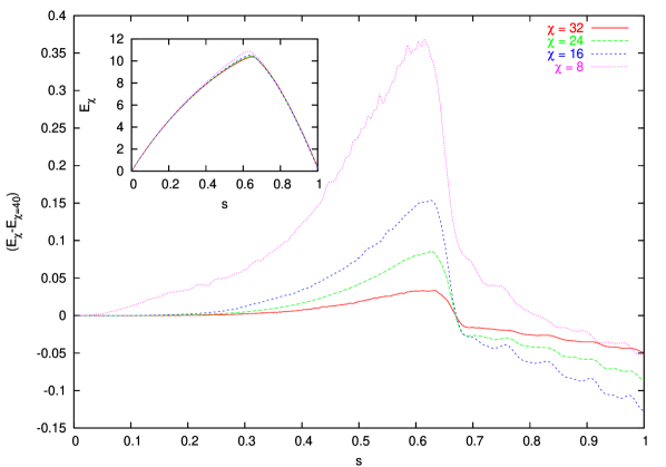
Figure 1: (Color online) Computation of the absolute error (compared to the $\chi=40$ case) of the expected value of the energy (cost function) along the adiabatic evolution for a typical instance with 30 qubits and 24 clauses for $T=100$ as $\chi$ increases. Note the increasing precision with larger $\chi$ as $s$ approaches the phase transition from the left-hand-side. In the inset, the absolute cost function is plotted. A similar behavior is also obtained for other instances, all of them getting the exact solution at the end of the computation.

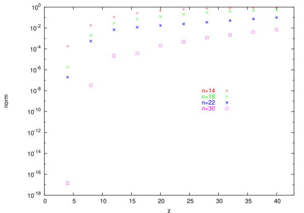
Figure 2: (Color online) Norm in the register as a function of $\chi$ in logarithmic scale, for instances of $14,18,22$ and $30$ qubits.

The error in the cost function is minimized as $\chi$ increases. It is noteworthy to observe how the error in the simulation of the adiabatic algorithm peakes at the phase transition point. We have also checked that it is precisely at this point where each qubit makes a decision towards its final value in the solution. Physically, the algorithm builds entanglement up to the critical point where the solution is singled out and, thereon, the evolution drops the superposition of wrong states in the register.

This success comes at the price of a controlled loss of unitarity. We plot in Fig. 2 the norm in the simulation as a function of $\chi$ in logarithmic scale, for instances of $14,18,22$ and $30$ qubits. The remarkable fact is that some observables, like the energy, appear to be very robust against this inaccuracy. Our simulations also allow to compute the decay of the $\chi$ Schmidt coefficients $\lambda^{(a)}_{\alpha}$ at any step of the computation. Close to criticality, and for the central cut of the system, these can be approximately fitted by the law $\log_{2}(\lambda^{(n/2)}_{\alpha})=b+\frac{c}{\sqrt{\alpha}}+d\sqrt{\alpha}$, with appropriate coefficients $b,c$ and $d$.

The ultimate goal of finding the correct solution appears also to be very robust in the simulations we have performed. The exact probability of success can be calculated in $O(n\ {\rm poly}(\chi))$ time as well. As a symbolic example, our program has solved an instance with $n=100$ qubits, that is, the adiabatic evolution algorithm has found the correct product state out of $2^{100}\sim 10^{30}$ for a hard instance with $m=84$ clauses and $T=2000$. The simulation was done with a remarkable small $\chi=14\ll 2^{50}=\chi_{max}$ and is presented in Fig. 3.

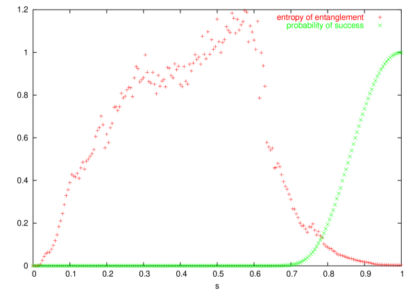
Figure 3: (Color online) An instance with $n=100$ qubits and $m=84$ clauses is solved using adiabatic evolution with $\chi=14$. The plot shows the entanglement entropy of a half-cut and the probability in solution state vs. $s$.

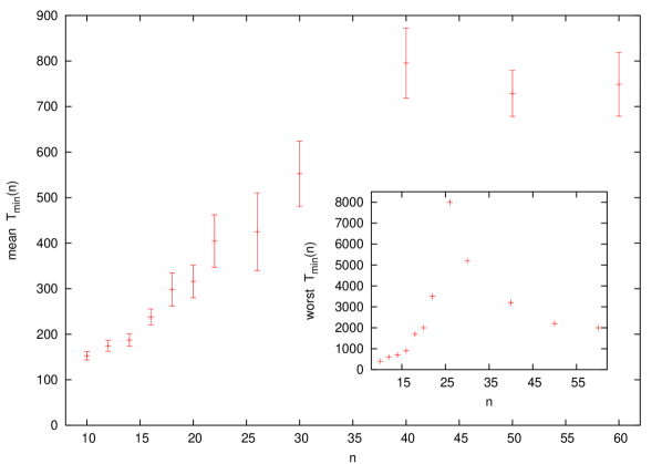
Figure 4: (Color online) Accumulated statistics up to $n=60$ for $T_{min}(n)$ for which each instance is solved (mean and worst cases). Averages are performed over $200$ instances for each $n$, except for $n=50,60$ with respectively $199,117$ instances. Error bars give $95$ per cent of confidence level in the mean. The worst cases found are shown in the inset.

The same robustness of evolving towards the correct solution is found for any number of qubits and small $\chi$. We have launched a search for the minimal $T$ that solves samples of $n$-qubit hard instances in the following way: for a set of small values of $\chi$, we try a random instance with an initial e.g. $T=100$. If the solution is found, we proceed to a new instance, and if not, we restart with a slower adiabatic evolution e.g. $T=200$. This slowing down of the algorithm is performed till a correct solution is found and the minimal successful $T_{min}$ is stored. Our results are shown in Fig. 4. The average over $n$-qubit instances appears to grow sub-exponentially with $n$. In fact, a quadratic fit reproduces the data for $n<22$, consistently with the results found in farhi . The required times for larger $n$ lie below the extrapolated curve. Isolated instances, however, may require larger times. Since the worst $T_{min}$ found depends on the interpolating path, finding an instance that needs a very large $T_{min}$ is no counterproof for the efficiency of the adiabatic algorithm, as alternative paths may solve the instance in a shorter $T$ farhi .

In this paper we have presented simulations of quantum computation based on matrix product states that can be taken up to 100 qubits. The remarkable fact that the algorithm finds the correct solution to a large hard instance and the robustness in the expected energy is to be contrasted with the loss of unitarity inherent to the local truncation scheme. This drawback may well be ameliorated if optimal truncations are implemented.

Acknowledgments: we acknowledge discussions with I. Cirac, E. Farhi and G. Vidal, and support from FPA2001-3598, GC2001SGR-00065, GVA2005-264 and FPA2002-00612. We would like to express our gratitude for the use of the GRID computing resources (GoG farm) and the support of computing technical staff of IFIC.

References

- (1) R. P. Feynman, Int. J. Theor. Phys. 21, 467 (1982).
- (2) A. Affleck, T. Kennedy, E.H. Lieb, H. Tasaki, Commun. Math. Phys. 115, 477 (1988); S. R. White, Phys. Rev. Lett. 69, 2863 (1992); M. Fannes, B. Nachtergaele, R. F. Werner, Commun, Math. Phys. 144, 443 (1992); S. Ostlund, S. Rommer, Phys. Rev. Lett. 75, 3537 (1995); J. Dukelsky, M. A. Martín-Delgado, T. Nishino, G. Sierra, Europhys. Lett. 43, 457 (1998); F. Verstraete, D. Porras, J. I. Cirac, Phys. Rev. Lett. 93, 227205 (2004).
- (3) G. Vidal, Phys. Rev. Lett. 91, 147902 (2003); G. Vidal, Phys. Rev. Lett. 93, 040502 (2004).
- (4) G. Vidal, J. I. Latorre, E. Rico, A. Kitaev, Phys. Rev. Lett. 90, 227902 (2003); J. I. Latorre, E. Rico, G. Vidal, Quant. Inf. and Comp. 4, 1 (2004).
- (5) F. Verstraete, J.I. Cirac, J.I. Latorre, E. Rico, M.M. Wolf, Phys. Rev. Lett. 94 140601 (2005).
- (6) F. Verstraete, J.I. Cirac, cond-mat/0407066.
- (7) E. Farhi, J. Goldstone, S. Gutmann, M. Sipser, quant-ph/0001106; E. Farhi, J. Goldstone, S. Gutmann, J. Lapan, A. Lundgren, D. Preda, quant-ph/0104129; E. Farhi, J. Goldstone, S. Gutmann, quant-ph/0208135.
- (8) M. R. Garey, D. S. Johnson, Computers and intractability; a guide to the Theory of NP-Completeness, W. H. Freeman and company, 1979.
- (9) A clause of Exact Cover is built from 5 clauses of 3-SAT, for which the transition is around . See J. M. Crawford, L. D. Auton, Artificial Intelligence 81:31-57 (1996).
- (10) T. Hogg, Phys Rev A 67 022314 (2003).
- (11) R. Orús, J. I. Latorre, Phys. Rev. A 69, 052308 (2004); J. I. Latorre, R. Orús, Phys. Rev. A 69, 062302 (2004).