The Quantum Mechanics of Hyperion

Abstract

This paper is motivated by the suggestion [W. Zurek, Physica Scripta, T76, 186 (1998)] that the chaotic tumbling of the satellite Hyperion would become non-classical within 20 years, but for the effects of environmental decoherence. The dynamics of quantum and classical probability distributions are compared for a satellite rotating perpendicular to its orbital plane, driven by the gravitational gradient. The model is studied with and without environmental decoherence. Without decoherence, the maximum quantum-classical (QC) differences in its average angular momentum scale as $\hbar^{2/3}$ for chaotic states, and as $\hbar^{2}$ for non-chaotic states, leading to negligible QC differences for a macroscopic object like Hyperion. The quantum probability distributions do not approach their classical limit smoothly, having an extremely fine oscillatory structure superimposed on the smooth classical background. For a macroscopic object, this oscillatory structure is too fine to be resolved by any realistic measurement. Either a small amount of smoothing (due to the finite resolution of the apparatus) or a very small amount of environmental decoherence is sufficient ensure the classical limit. Under decoherence, the QC differences in the probability distributions scale as $(\hbar^{2}/D)^{1/6}$, where D is the momentum diffusion parameter. We conclude that decoherence is not essential to explain the classical behavior of macroscopic bodies.

I Introduction

Quantum mechanics (QM) is a more fundamental theory than is classical mechanics (CM). This fact does not diminish the utility of CM in describing the behavior of macroscopic objects. But theoretical consistency demands that the observed classical phenomena should also emerge from QM in an appropriate limit. However, a detailed understanding of this quantum-to-classical (QC) limit is remarkably difficult to achieve, and the origin of classical behavior is even subject to a degree of controversy. There has been some confusion as to which QM structures should be compared with classical predictions, and hence to what the appropriate criterion for classicality should be. The role that decoherence due to environmental perturbations might play in establishing the QC limit is also controversial.

A criterion for classicality that has often been used is based on Ehrenfest’s theorem Ehrenfest (1927). If the size of the quantum state is small compared to the scale on which the potential energy varies, then the centroid of the state will approximately follow a classical Newtonian trajectory. The time duration (and range of other relevant parameters) within which this condition holds is referred to as the Ehrenfest regime. Since any wave packet will eventually spread until it reaches the size of the system (harmonic oscillators being a unique exception), it follows that this criterion for classicality will eventually fail, no matter how macroscopic the system may be. If the break time when this occurs were as long as the age of the solar system, there would be no cause for concern. But in chaotic systems, the size of a wave packet grows exponentially, and the break time can be quite small. A striking example, given by Zurek Zurek (1998), is the chaotic tumbling of Hyperion (a moon of Saturn), for which the Ehrenfest criterion for classicality will fail in less than 20 years. Zurek argues that environmental decoherence can remove this paradox and restore classical behavior to Hyperion. This claim is certainly not correct, as long as the Ehrenfest criterion for classicality is used. However, we propose another criterion for classicality, within which the role of decoherence will be reassessed.

The origin of the above paradox consists in a failing to take proper account of the statistical nature of QM. It is not correct to identify the trajectory of a body with the motion of the centroid of the wave function. QM does not describe the actual observed phenomenon, but only the probabilities of the various possible phenomena. We should, therefore, compare quantum probabilities with classical probabilities. This leads us to define the Liouville regime of quantum- classical correspondence, within which the quantum probabilities are approximately equal to the classical probabilities that satisfy the Liouville equation. There is no requirement that the probability distributions be narrow, and so the Liouville regime of classicality is usually much larger than the Ehrenfest regime.

The superiority of the Liouville criterion for classicality to the Ehrenfest criterion has been demonstrated in several ways. One way to see this is through the correction terms to Ehrenfest’s theorem. When the width of the state is small but not negligible, these corrections can be obtained as a series involving the variance and higher moments of the position probability distribution Ballentine et al. (1994). This series has exactly the same form for the classical Liouville probability distribution. Hence Ehrenfest’s theorem merely asserts that if the (quantum or classical) probability distribution is sufficiently narrow, its centroid will follow a Newtonian trajectory. To leading order, the deviations from the Newtonian trajectory are the same in both the quantum and classical cases, and so those deviations are not primarily quantal in origin. The magnitude of the deviations from Ehrenfest’s theorem depends primarily on the width of the initial state in configuration space, and has no systematic dependence on $\hbar$ Ballentine and McRae (1998). However, the (much smaller) differences between the quantum and classical probabilities scale as $\hbar^{2}$, indicating that they are truly of quantal origin.

Our interest in Hyperion was stimulated by Zurek’s provocative paper Zurek (1998). He begins with an estimate of the break time, $T_{E}$, beyond which the Ehrenfest criterion of classicality will fail. Since the width of a wave packet in a chaotic system grows exponentially with the Lyapunov exponent $\lambda$, the time taken for it to reach the scale $L$ over which the potential varies (typically of order of the system size) will be $T_{E}=\lambda^{-1}\ln(L/\Delta x_{0})$, where $\Delta x_{0}$ is the initial width of the wave packet. Zurek chooses $\Delta x_{0}=\Delta p_{0}/\hbar$, with the width of the momentum distribution $\Delta p_{0}$ being estimated from thermal fluctuations, and thereby obtains the now-familiar result that the break time $T_{E}$ scales as $\ln(\hbar^{-1})$. This $T_{E}$ can be quite short, even for a macroscopic system, and because of the logarithmic dependence, it is not sensitive to detailed assumptions about the initial state. Thus, according to the Ehrenfest criterion for classicality, the tumbling motion of Hyperion should long ago have ceased to be classical.

This paradoxical conclusion is not affected by including environmental decoherence. Decoherence converts a pure state into a mixed state, but it does not produce localization of the position probability density, and so it has no significant influence on the breakdown of Ehrenfest’s theorem. (Indeed, the diffusive term that describes the effect of the environment in the master equation for the density matrix will have a slight delocalizing effect.) Therefore, if the Ehrenfest criterion were the sole criterion for classicality, we would still be faced with the paradoxical conclusion that macroscopic bodies like Hyperion should be grossly non-classical.

In Zurek and Paz ; Zurek (1998) Zurek next considers the equation of motion of the Wigner function, which has the form of the classical Liouville equation plus a series of $\hbar$-dependent terms, called the Moyal terms. The limit of the Liouville regime of classicality will presumably be reached when the Moyal terms have a significant effect. Unfortunately, Zurek does not distinguish between the Ehrenfest and Liouville regimes, and denotes both break times as $t_{\hbar}$. This is a serious confusion, since they are both conceptually and numerically distinct.

While the time limit $T_{E}$ of the Ehrenfest regime is easy to estimate reliably, an analogous limit for the Liouville regime is much more difficult to obtain. Zurek uses heuristic arguments to claim that decoherence tends to counter the effects of the Moyal terms, and he obtains a Liouville break time similar in form to $T_{E}$ Zurek and Paz . We consider this conclusion to be doubtful for several reasons. Habib et al. Habib et al. (2002) have shown that, in order for the non-negativity of the density matrix (“rho-positivity” in their terminology) to be preserved, the Moyal terms must have subtle effects that are not counteracted by decoherence. Full numerical computations for a driven system Emerson and Ballentine (2000) and for an autonomous system Ballentine (2004) have found that, although the differences between quantum and classical averages of observables have a brief period of exponential growth, these differences reach a saturation value, about which they fluctuate irregularly. This saturation value is much smaller than the system size (unlike the deviations from Ehrenfest’s theorem), and it tends to zero as some small power of $\hbar$. The break time estimated by Zurek would be relevant only if the exponential growth of these QC differences continued until they reached macroscopic size.

In this paper we perform classical and quantum computations for the chaotic tumbling of an object like Hyperion, which complement the published classical theory Wisdom (1987). The actual value of the de Broglie wavelength is, of course, much too short to be treated in a numerical integration of the Schrödinger equation. So we cast the equation into dimensionless form, and solve it for a range of the dimensionless $\hbar$ parameter. These results lead to scaling relations, from which we can extrapolate to estimate the values appropriate to Hyperion. We study the system with and without environmental decoherence, discuss the conditions needed to ensure classicality, as well as examine whether there is a qualtiative difference between the classical limit of regular and chaotic initial states.

II Model

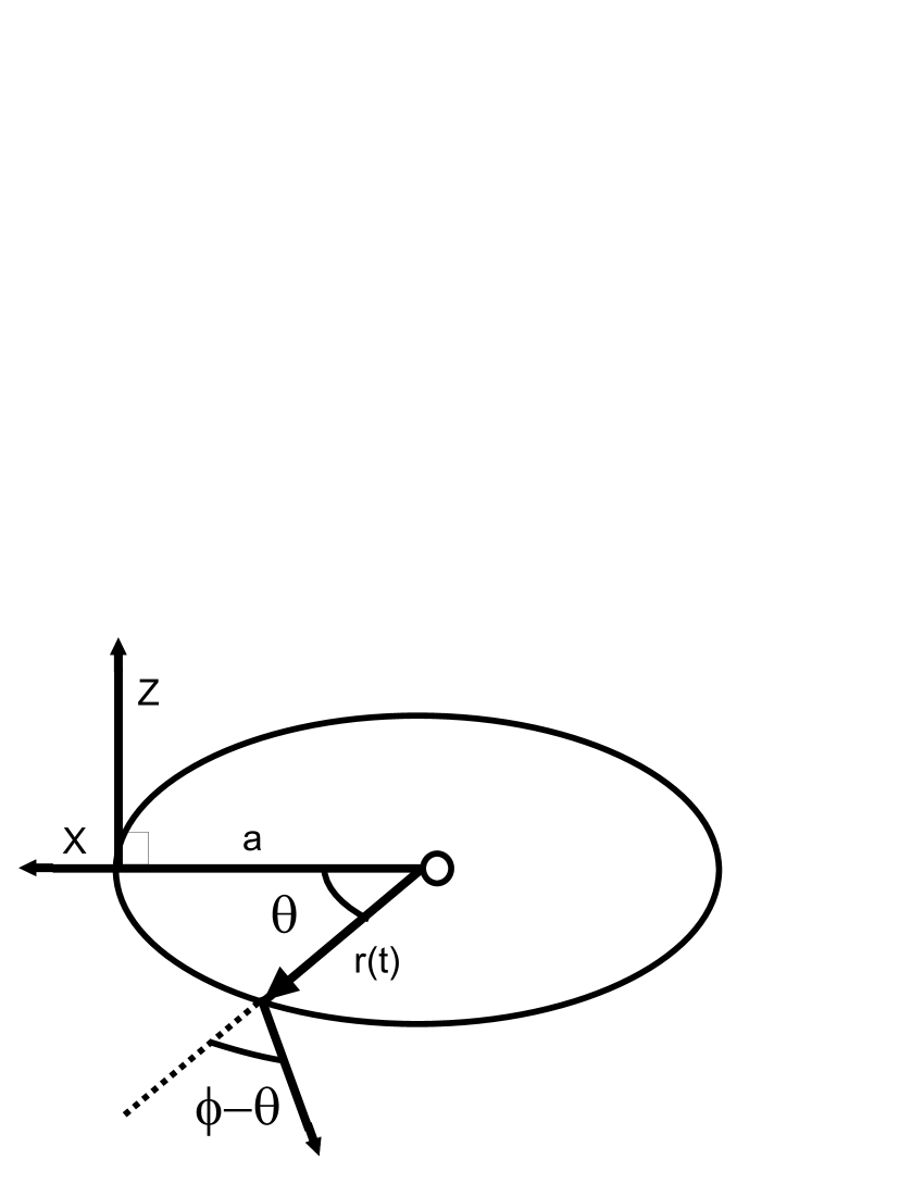
Figure 1: Orbit of satellite spinning about the z-axis perpendicular to the orbital plane. $\theta$ denotes the position of the satellite on the orbit, and $\phi$ is the orentation of the satellite with respect to the semi-major axis of the orbit.

Our model of Hyperion’s rotation was first suggested in 1988 by Wisdom Wisdom (1987). It assumes that Hyperion’s center of mass travels in an elliptical orbit about Saturn, and that its orbit is unaffected by its rotation. However, since Hyperion is an extended object, Saturn’s gravitational field is not constant over its volume. Since its mass distribution is not spherical, the variation in the gravitational field can produce a net torque. To lowest order in a multipole expansion of the mass distribution, this torque depends on the quadrupole moment of the mass distribution, and for simplicity we neglect all higher order moments.

It should be noted that this configuration is attitude unstable, and so small inclinations of $I_{3}$ towards the plane of the orbit will tend to grow. However this simplifying assumption makes both the classical and the quantum mechanical computations feasible.

The coordinate system is shown in Fig. 1. The space-fixed x-axis is along the semi-major axis of the orbital ellipse, and the z-axis is perpendicular to the orbital plane. The angle $\theta$ denotes the position of the satellite in the orbit. The axis of the smallest moment of inertia ($I_{1}$), makes an angle $\phi$ with respect to the x-axis, hence the angle between the body axis of $I_{1}$ and the radius vector $\vec{r}$ is $\phi-\theta$. The largest moment of inertia $I_{3}$ is parallel to the z-axis. The canonical coordinates for this system are the angular momentum and the orientation of the satellite $\{L_{z},\phi\}$.

The coupling of the gravitational field to the satellite is obtained by a Taylor expansion of the potential about the satellite’s center of mass,

$$H=\frac{L_{z}^{2}}{2I_{zz}}+\left.\sum_{i}\sum_{j}\int\rho(\vec{r})x_{i}x_{j}d^{3}x\frac{\partial^{2}V}{\partial x_{i}\partial x_{j}}\right|_{\vec{x}=0}+\cdots$$ (1)

Here $x_{i}$ refers to the distance along the $i$’th space-fixed axis from the center of mass of the satellite.

$$\left.\frac{\partial^{2}V}{\partial x_{i}\partial x_{j}}\right|_{\vec{x}=0}=diag\left[\frac{2Gm}{r^{3}},\frac{-Gm}{r^{3}},\frac{-Gm}{r^{3}}\right]$$ (2)

Here m is the mass of the gravitational source (Saturn), and r is the distance from the source to the satellite. The first order term in Eq. (1) vanishes because the expansion is about the center of mass, and the second order term is related to the moments of inertia tensor,

$$I_{ij}=\int\rho[x^{2}\delta_{ij}-x_{i}x_{j}]d^{3}x$$ (3)

Using Kepler’s third law, which states $GM/a^{3}=4\pi^{2}/T^{2}$,‘ the Hamiltonian becomes

$$H=\frac{L_{z}^{2}}{2I_{3}}-\frac{3\pi^{2}}{T^{2}}\left(\frac{a}{r(t)}\right)^{3}(I_{2}-I_{1})\cos(2[\phi-\theta(t)])$$ (4)

Here $T$ is the orbital period, $a$ is the length of the semi-major axis of the orbit, $L_{z}$ is the angular momentum about the z-axis, $I_{3}=I_{zz}$ is the moment of inertia for rotations in the orbital plane, and r(t) and $\theta(t)$ are the orbital coordinates of the satellite, which are functions of the period $T$ and the eccentricity $e$. These functions are found by numerically integrating the equations of motion for the center of mass, using the code provided in Caroll and Ostlie (1996).

II.1 Classical Equation Of Motion

It is convenient to express the equation of motion in terms of dimensionless variables. We introduce the anisotropy parameter,

$$\alpha=\frac{(I_{2}-I_{1})}{I_{3}}$$ (5)

a dimensionless time (in units of the orbital period),

$$\tau=t/T$$ (6)

and a dimensionless angular momentum $J_{z}$ in terms of the dimensional angular momentum $L_{z}$

$$J_{z}=\frac{L_{z}T}{I_{3}}$$ (7)

To estimate $\alpha$ for Hyperion, we use the observed lengths of its principle axes (410 $\pm$ 10, 260 $\pm$ 10, 220 $\pm$ 10 km) Thomas et al. (1983), and assume that it is an ellipsoid of uniform mass density. Hence

$$I_{3}=\frac{M}{5}(r_{1}^{2}+r_{2}^{2})$$ (8)

Here $r_{i}$ is half the length of the $i^{th}$ principle axis of the ellipsoid. The other moments of inertia are obtained by cyclically permuting the indices. Substituting Eq. (8) into Eq. (5) yields

$$\alpha=\frac{r_{1}^{2}-r_{2}^{2}}{r_{1}^{2}+r_{2}^{2}}$$ (9)

Hence $\alpha=0.43\pm 0.04$. In this work we used a slightly larger value, $\alpha=0.5$, because it leads to a more purely chaotic motion, whereas for $\alpha=0.43,e=0.1$ there are large regular islands embedded in the chaotic sea. We wish to compare chaotic motions with regular motions, and the differences would be obscured by a mixed phase space.

Following Wisdom Wisdom (1987), we obtain the equation of motion (in dimensionless variables) to be

$$\dot{\phi} = J_{z}$$

$$\dot{J_{z}} = -6\pi^{2}\left(\frac{a}{r(\tau)}\right)^{3}\alpha\sin(2[\phi-\theta(\tau)])$$ (10)

II.2 Quantum Mechanics

The quantum mechanics will be solved by integrating the Schrödinger equation in angular momentum representation. The state vector is written as

$$|\psi(t)\rangle=\sum_{m}c_{m}(t)|m\rangle,$$ (11)

with $|m\rangle$ being an angular momentum eigenstate. The matrix elements of the Hamiltonian are

$$\langle m|\hat{H}|\psi\rangle=\frac{\hbar^{2}m^{2}c_{m}}{2I_{3}}-\sum_{n}\frac{3\pi^{2}}{2T^{2}}c_{n}\left(\frac{a}{r(t)}\right)^{3}\times$$

$$(I_{2}-I_{1})\frac{1}{2\pi}\int_{0}^{2\pi}(e^{i(n-m+2)\phi}e^{-2i\theta}+e^{i(n-m-2)\phi}e^{2i\theta})d\phi$$

(12)

Using (12) and (11), the matrix equation $\langle m|\hat{H}|\psi\rangle=i\hbar\langle m|\frac{\partial}{\partial t}|\psi\rangle$ becomes

$$i\hbar\frac{\partial c_{m}(t)}{\partial t}=\frac{\hbar^{2}m^{2}c_{m}}{2I_{3}}-\frac{3\pi^{2}}{2T^{2}}\left(\frac{a}{r}\right)^{3}(I_{2}-I_{1})\times$$

$$(c_{m+2}e^{2i\theta(t)}+c_{m-2}e^{-2i\theta(t)})$$ (13)

In addition to the dimensionless parameters $\tau$ and $\alpha$, we now introduce a dimensionless $\hbar$ parameter,

$$\beta=\frac{\hbar T}{I_{3}}$$ (14)

The dimensionless Schrödinger equation then becomes

$$i\frac{\partial c_{m}}{\partial\tau}=\frac{\beta m^{2}c_{m}}{2}-\frac{3\pi^{2}}{2}\frac{\alpha}{\beta}\left({\frac{a}{r(\tau)}}\right)^{3}\times$$

$$(c_{m+2}e^{2i\theta(\tau)}+c_{m-2}e^{-2i\theta(\tau)})$$ (15)

A peculiar feature of Eq. (15) is that the coefficient $c_{m}$ depends only on $c_{m+2}$ and $c_{m-2}$, therefore the even $c_{m}$ cannot interact with odd $c_{m}$. This coupling arises from the invariance of the Hamiltonian under rotations by $\pi$. But octapole and other odd moments are not invariant under rotations by $\pi$, so this symmetry is an artifact of the model.

II.3 Initial State

The initial quantum state is chosen to be a Gaussian in angular momentum,

$$|\psi\rangle=\sum_{m}\exp\left(-\frac{(\beta m-J_{0})^{2}}{2\delta^{2}}-i\phi_{0}m\right)|m\rangle$$ (16)

Here $\beta m$ is a dimensionless angular momentum, $J_{0}$ is the average of the dimensionless angular momentum in the state, $\delta$ is its standard deviation, and $\phi_{0}$ is the central angle of the initial state. These parameters will be varied to ensure that the initial states are in regions of phase space that are either purely chaotic or purely regular.

In principle the sum is from $m=-\infty$ to $+\infty$, but in practice it is restricted to a range $\{-K\cdots K\}$. The value of $K$ must be chosen so that this range includes all of the values of $J_{z}$ that have significant amplitudes in the time-dependent state. By examining phase-space diagrams for the classical distributions, we found that $|J_{z}|<20$ for all time, and so $K=20/\beta$ was sufficient to contain the quantum distribution.

The initial classical probability distributions are chosen so that they match the angular momentum and angular distributions for the initial quantum state. Because the initial state is a minimum uncertainty state with fixed width in angular momentum, its width in angle is proportional to $\beta$. Thus $\beta$ (dimensionless $\hbar$) enters into the classical calculation to ensure that the initial quantum and classical states correspond to each other.

III Results For A Non-Chaotic State

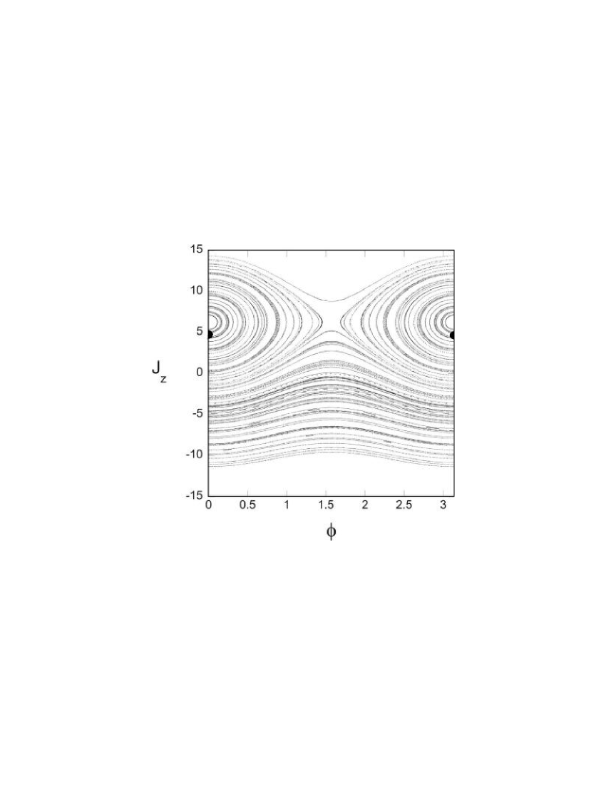
Figure 2: Poincare Section for $e=0$, $\alpha=0.5$. Black circle denotes a typical initial state.

The classical limit of the quantum tumbling of a satellite will now be examined for a non-chaotic state, to determine whether there is a qualitative difference between chaotic and non-chaotic systems in their approach to classicality.

Non-chaotic motion is ensured by choosing a circular orbit: $e=0$, $r(\tau)=a$, $\theta(\tau)=2\pi\tau$. The time dependence in Eq. (10) can be transformed away by the substitution $\Phi=\phi-2\pi\tau$, yielding an integrable equation of motion,

$$\ddot{\Phi}=-6\pi^{2}\alpha\sin(2\Phi)$$ (17)

Fixed points for this equation occur at the angles $\Phi=0,\frac{\pi}{2},\pi,\frac{3\pi}{2}$. These fixed points describe motions in which Hyperion presents the same face to Saturn at all times. The stable fixed points correspond to the smallest moment of inertia pointing towards Saturn.

The initial state was chosen to be far from the unstable fixed point. It is centered at $J_{0}=4$, with a standard deviation in $J_{z}$ of $\sigma=\frac{1}{\sqrt{2}}$ (see Fig. 2), and a central anglei $\phi_{0}$ equal to zero.

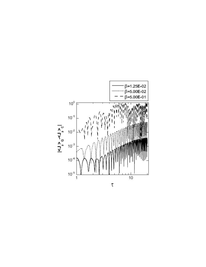
Figure 3: QC differences in $\langle J_{z}\rangle$ vs $\tau$, for several $\beta$, with $e=0$, $\alpha=0.5$. For $\beta=\{0.0125,0.05,0.5\}$ the statistical errors are $\sigma_{m}=\{0.0002,0.0007,0.002\}$.

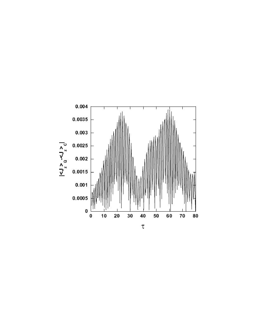
Figure 4: QC differences in $\langle J_{z}\rangle$ for $\beta=0.0125$, with $e=0$, $\alpha=0.5$, $\sigma_{m}=0.7\times 10^{-3}$

.

III.1 QC Differences in $\langle J_{z}\rangle$

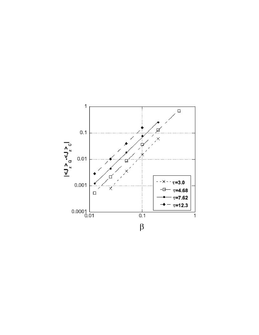
Figure 5: Scaling of the early time QC differences in $\langle J_{z}\rangle$ with $\beta$, for $e=0$, $\alpha=0.5$. Showing a $\beta^{2}$ dependence.

The classical probability distributions are found by time evolving a finite ensemble of systems, using Eq. (10). The distributions of $J_{z}$ and $\phi$ are found by randomly choosing the angular momentum and orientation of each member of the ensemble from probability distributions in $J_{z}$ and $\phi$ that correspond to the initial quantum state.

The finiteness of the ensemble leads to statistical errors, which may be reduced by increasing its size. The standard deviation of the fluctuations in the mean is

$$\sigma_{m}=\frac{\sigma}{\sqrt{n}}$$ (18)

Here $n$ is the number of members in the ensemble, $\sigma$ is the standard deviation of the distribution. Any difference between the computed mean values of the quantum and the classical variables is not significant unless it is larger than $\sigma_{m}$. Ensembles of 1,000,000 to 20,000,000 particles were used to ensure that the typical QC differences are greater than $\sigma_{m}$.

As $\beta\rightarrow 0$ the QC differences become smaller, and thus a larger ensemble is needed to reduce the statistical errors below that level. Hence different ensemble sizes were used for different values of $\beta$ in Fig. 3. The ensemble sizes were chosen so that $\sigma_{m}=\{0.0002,0.0007,0.002\}$ for $\beta=\{0.0125,0.05,0.5\}$.

Ensembles were evolved for several values of $\beta$, ranging from $\beta=0.5$ to $\beta=0.002$. For $\beta<0.01$ the QC differences were far smaller than $\sigma_{m}$ for any computationally feasible ensemble sizes, so no data will be presented for $\beta<0.01$.

A plot of the QC differences in $\langle J_{z}\rangle$ is shown in Fig. 3. In this and similar figures, any QC differences smaller than $\sigma_{m}$ should be ignored, since they are dominated by statistical errors. The QC differences oscillate on the scale of the driving force, and only the envelope of these oscillations is of interest. From Fig. 3 it is apparent that at early times the envelope of the QC differences grows as $\tau^{2}$. For longer times the envelope of the QC differences is oscillatory, as can be seen in Fig. 4. Such recurrences are typical for non-chaotic systems Haake (2001). Fig. 5 shows that, for fixed times, the QC differences in $\langle J_{z}\rangle$ scale as $\beta^{2}$. This result is similar to that found for some other systems Ballentine and McRae (1998).

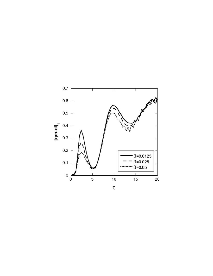
Figure 6: Variation of $|qm-cl|_{1}$ [Eq. (19)] with time and $\beta$ for the nonchaotic state ($e=0$, $\alpha=0.5$). Each classical ensemble has 1,000,000 members.

III.2 QC Differences in Distributions

The differences in $\langle J_{z}\rangle$ alone are insufficient to fully describe the differences between quantum and classical systems because two different probability distributions can have the same mean but different variances and higher moments. We shall now examine the differences between probability distributions, and how they scale with $\beta$.

Since the angular momentum distributions are discrete, one can regard them as vectors, and measure the difference between the quantum and classical probability vectors by the 1-norm, defined as

$$|qm-cl|_{1}=\sum_{m}|P_{cl}(m)-P_{qm}(m)|$$ (19)

This probability distribution is normalized so that $\sum_{m}P(m)=1$. Alternatively, one can define a probability density, which is normalized so that $\int\tilde{P}(\hbar m)d(\hbar m)=1$. Then the 1-norm of the probability densities takes the form

$$|qm-cl|_{1}=\int_{-\infty}^{\infty}|\tilde{P}_{cl}(\hbar m)-\tilde{P}_{qm}(\hbar m)|d(\hbar m)$$ (20)

These two forms are equivalent because $\tilde{P}(\hbar m)=P(\hbar m)/\hbar$, and the additional factor of $\hbar$ is cancelled by the factor of $\hbar$ in the integral.

Fig. 6 shows that the QC differences in the probability distributions do not tend to zero as $\beta\rightarrow 0$. This lack of pointwise convergence of the quantum probability distributions to the classical limit has also been observed for other systems, such as a particle in a box and the kicked rotor Ballentine (1999). In these one-dimensional driven system, the quantum probability distributions develop a fractal-like structure, and only the smooth background converges to the classical probability distribution. We will show in section V.3 that a similar result holds for Hyperion.

IV Results For a Chaotic State

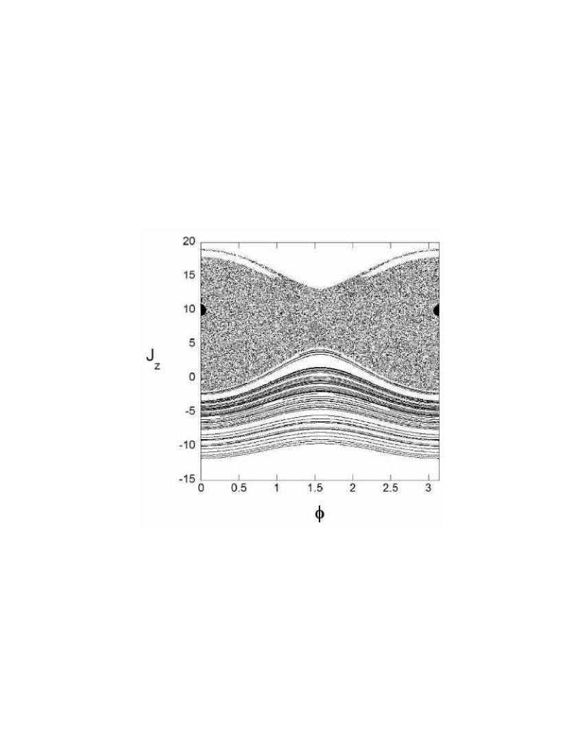
Figure 7: Poincare Section for a chaotic state, $\alpha=0.5$, $e=0.1$. Black circle denotes a typical initial state, with $J_{z}=10$ and $\delta=0.5$

In this section the rotation of a satellite is investigated for a chaotic state. The previous value of $\alpha=0.5$ is used, but now the eccentricity is taken to be Hyperion’s value of $e=0.1$. The computation is carried out as in section III.

The initial state is centered at dimensionless angular momentum $J_{0}=10$, with a standard deviation of $\sigma=0.5$, and a central angle $\phi_{0}=0$. This state is in the chaotic sea, far away from any regular torii, as can be seen in Figure 7. The maximum Lyapunov exponent for the chaotic sea is $\lambda=0.85$.

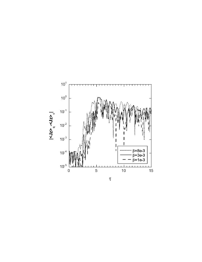
Figure 8: QC differences in $\langle J_{z}\rangle$ vs $\tau$ for a chaotic state, $\alpha=0.5,e=0.1$. For $\beta=\{1\times 10^{-3},3\times 10^{-3},8\times 10^{-3}\}$ the statistical errors are $\sigma_{m}=\{1.4\times 10^{-4},1.4\times 10^{-4},2.2\times 10^{-4}\}$.

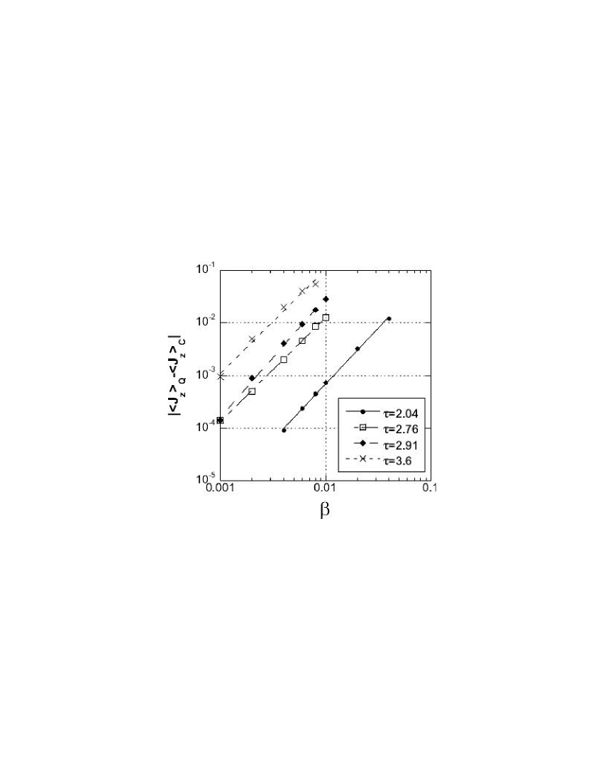
Figure 9: QC differences in $\langle J_{z}\rangle$ vs $\beta$, for a chaotic state before saturation is reached, showing a $\beta^{2}$ dependence.

This state was evolved for several periods of the driving force, and the differences between the quantum and classical results were computed. In Fig. 8 the QC differences in $\langle J_{z}\rangle$ are initially dominated by statistical errors, which are approximately $\sigma_{m}=2\times 10^{-4}$. The QC differences in $\langle J_{z}\rangle$ grow exponentially with time until they saturate at $\tau\approx 6$. This saturation occurs when the classical trajectories ergodically fill the chaotic sea. For $\tau>20$ the classical ensemble saturates at $\langle J_{z}\rangle\approx 8.2$. The quantum value of $\langle J_{z}\rangle$ also saturates at approximately the same value, but with irregular fluctuations superimposed. This suggests that the QC differences here are dominated by quantum fluctuations, once the probability distributions have saturated the chaotic sea.

IV.1 QC Differences in $\langle J_{z}\rangle$ for Early Times

To determine how the QC differences scale with $\beta$, we varied $\beta$ with $\tau$ fixed at the times of the peaks in Fig. 8. From Fig. 9 it can be seen that the QC differences in $\langle J_{z}\rangle$ scale as $\beta^{2}$; the same scaling as was found for the non-chaotic states. This $\beta^{2}$ scaling was previously found by a different method for other systems Ballentine and McRae (1998). The classical ensemble sizes were chosen so that $\sigma_{m}=\{1.6\times 10^{-4},1.6\times 10^{-4},2.2\times 10^{-4}\}$ for $\beta=\{1\times 10^{-3},3\times 10^{-3},8\times 10^{-3}\}$.

In the initial growth region of Fig. 8,the QC differences in $\langle J_{z}\rangle$ vary with time as

$$|\langle J_{z}\rangle_{Q}-\langle J_{z}\rangle_{C}|\propto e^{2.9\tau}$$ (21)

for $\tau=2$ between 2 and 5.5. The exponent in Eq. (21) appears to be independent of the value of $\beta$. The exponent is greater than $2\lambda$, implying that the QC differences grow at a rate that is greater than the classical Lyapunov exponent. Similar results have been obtained for some other systems Ballentine and McRae (1998); Ballentine (2002); Emerson and Ballentine (2000).

The exponential growth eventually saturates. This cessation of exponential growth of the QC differences in $\langle J_{z}\rangle$ is relevant to Zurek’s argument Zurek (1998) that, absent decoherence, the QC differences for Hyperion should reach macroscopic size within about 20 years. That argument implicitly assumes that the QC differences will continue to grow exponentially until they reach the size of the system. However, we find that not to be the case.

IV.2 QC Differences in $\langle J_{z}\rangle$ for the Saturation Regime

The maximum QC differences occurs in the saturation regime. If these differences converge to 0 as $\beta\rightarrow 0$ then the classical limit will be reached for all times, and there will be no break time beyond which QC correspondence fails.

At the beginning of the saturation region (Fig. 8 and Fig. 15), the QC differences in $\langle J_{z}\rangle$ reach a maximum, before decaying to a saturation level, about which they fluctuate irregularly. Because of this fluctuation in the saturation regime, we calculate the time average of the QC differences. Here $|\langle J_{z}\rangle_{Q}-\langle J_{z}\rangle_{C}|$ was averaged over $\tau$ from 20 to 100. As shown in Figure 11, these averaged QC differences tend to scale as $\beta^{2/3}$.

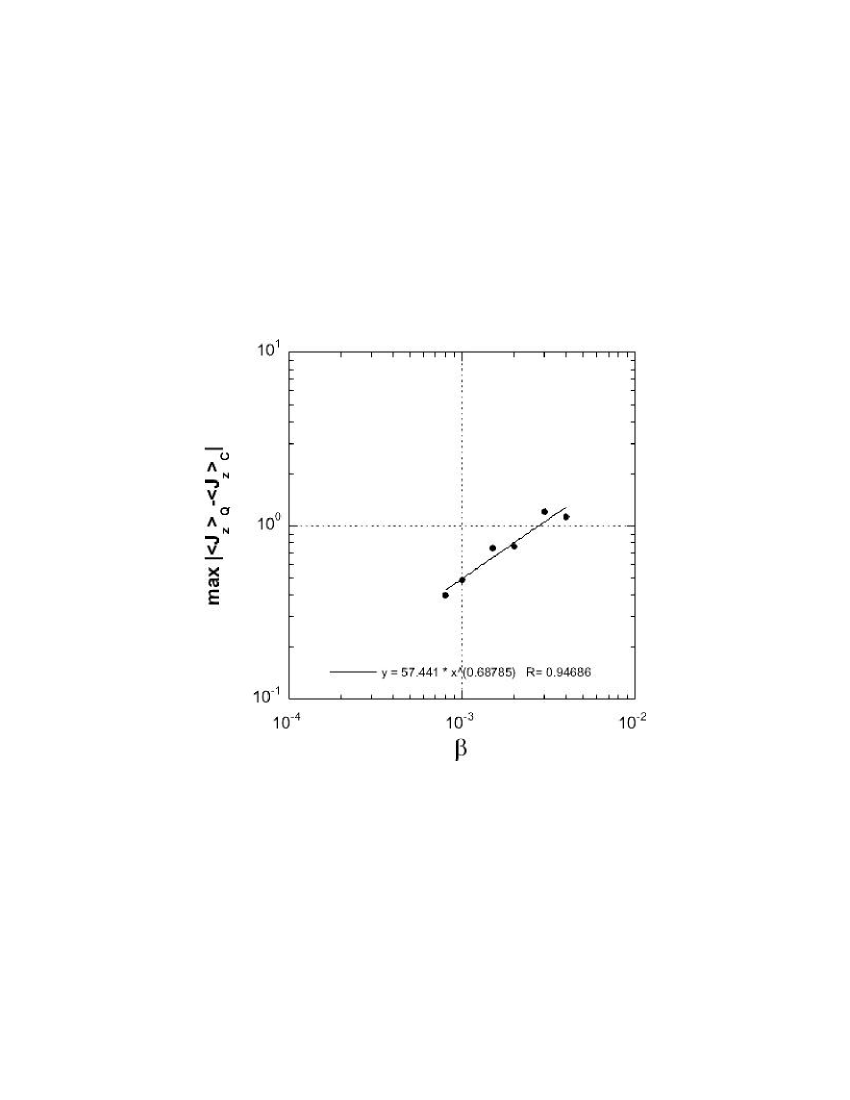
Figure 10: Maximum QC differences in $\langle J_{z}\rangle$ versus $\beta$ for a chaotic state. $e=0.1$, $\alpha=0.5$. Suggests that this maximun difference scales as $\beta^{2/3}$.

For sufficiently small $\beta$, the peak QC differences also scales as $\beta^{2/3}$ (see Fig. 10). This scaling also was found for the maximum QC differences in a model of coupled pendulums Ballentine (2004), so it might be generic for chaotic systems in the saturation regime.

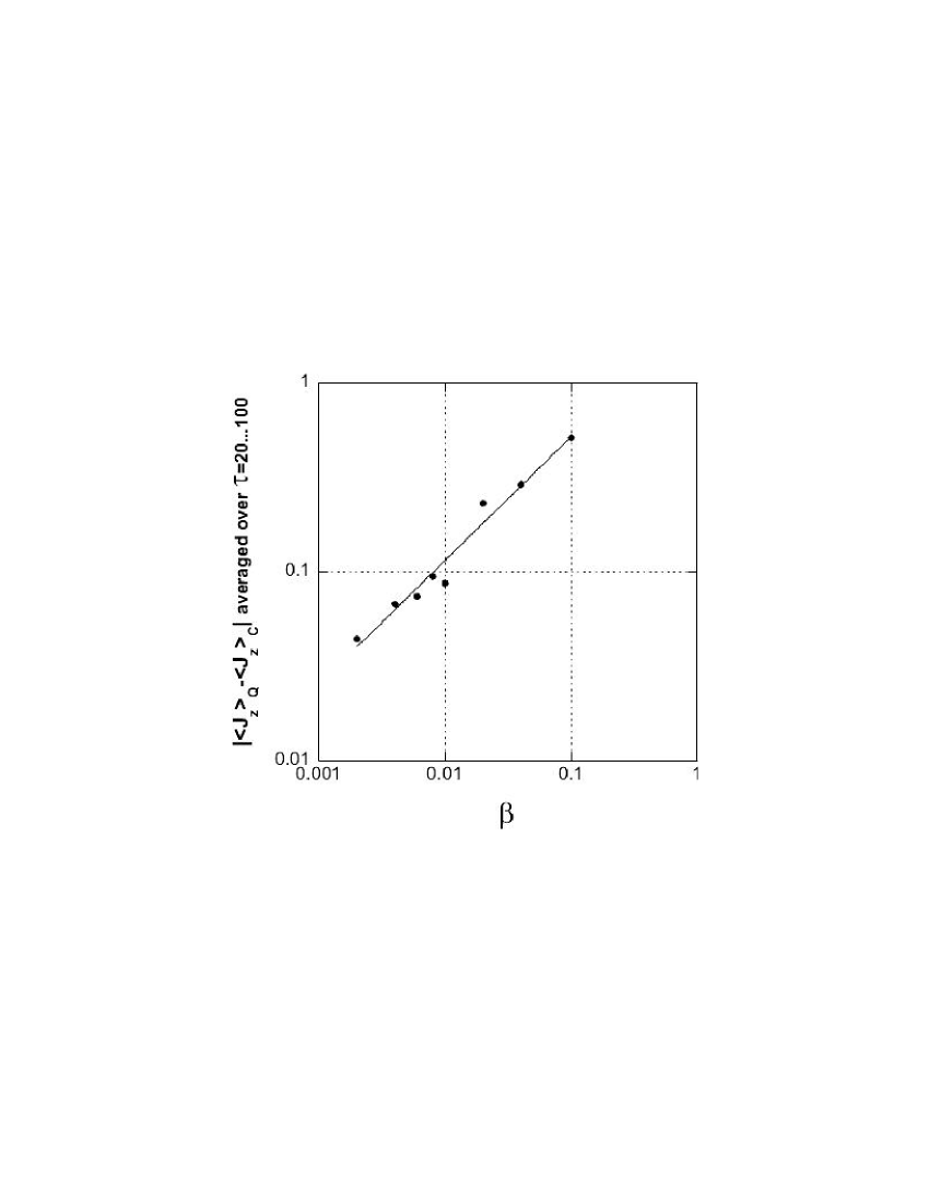
Figure 11: QC differences in $\langle J_{z}\rangle$, averaged over $\tau$ from $20$ to $100$. Initial state is in the chaotic sea. $e=0.1$, $\alpha=0.5$. Suggests that $\langle|\langle J_{z}\rangle_{Q}-\langle J_{z}\rangle_{C}|\rangle\propto\beta^{2/3}$ in the saturation regime.

IV.3 QC Differences in Probability Distributions

The probability distributions contain much more information than do the averages of observables. These probability distributions are shown in Figures 12 and 19. We use the quantity $|qm-cl|_{1}$ (defined in Eq. (19)) as a measure of the QC differences in the probabilities.

As can be seen from Fig. 14, $|qm-cl|_{1}$ increases with time before saturating, but fails to converge to 0 as $\beta\rightarrow 0$. Since pointwise convergence does not occur, neither for the chaotic nor for the non-chaotic states, this lack of pointwise convergence is not a result of chaos.

Most of the QC differences in the probabilities occur on a very fine scale, and a modest amount of smoothing is sufficient to cause the quantum probability distributions to better approximate the classical results. Fig. 13 shows that the differences between the two distributions are dramatically reduced by smoothing them over a small width. This smoothing process is discussed and compared to environmental decoherence in section V.3.

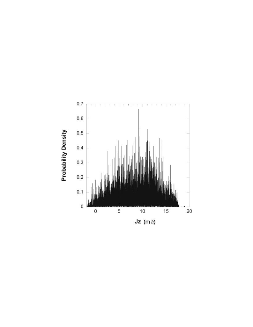
Figure 12: Quantum probability density for $\tau=40.0$, $\beta=0.002$

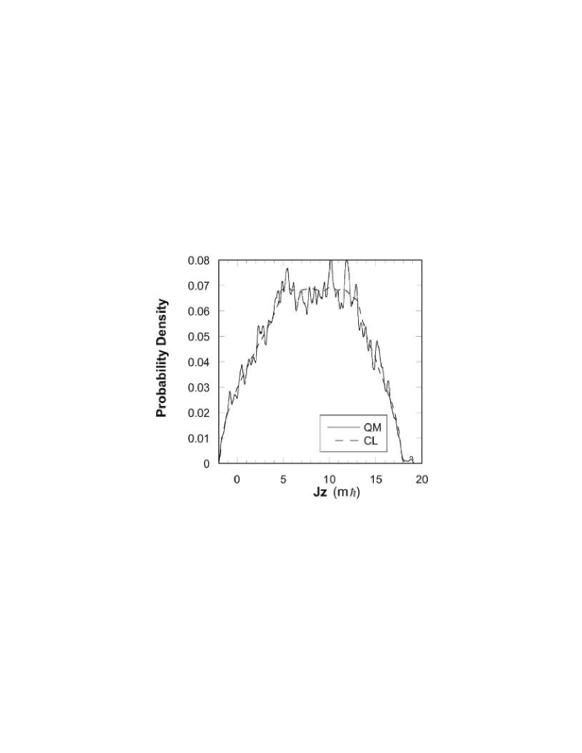
Figure 13: Quantum and classical probability densities for $\tau=40.0$, $\beta=0.002$. Both quantum and classical densities are convolved with a triangular filter of width $0.25$ in $J_{z}$

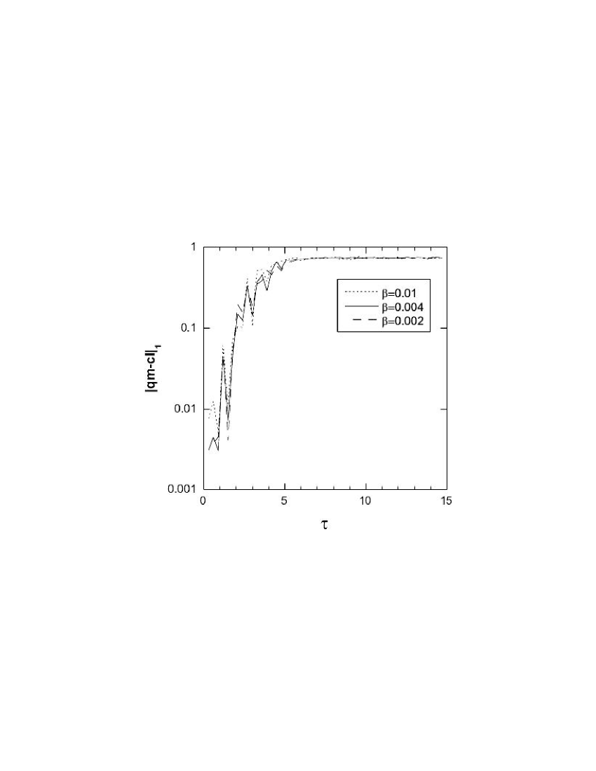
Figure 14: $|qm-cl|_{1}$ vs time for different values of $\beta$, for a chaotic state, $e=0.1$

To summarize the results of this section, for early times the QC differences in $\langle J_{z}\rangle$ scale as $\beta^{2}$, and increase exponentially with time. The exponential growth ceases when the probability distributions saturate the chaotic sea. Both the maximum values and the saturation levels of the QC differences were found to scale as $\beta^{2/3}$. A small amount of smoothing can dramatically reduce the QC differences in the probability distributions, since most of the differences come from very fine scale structures in the quantum probability distributions.

V Environmental Effects

Interaction with the environment leads to decoherence and dissipation. Decoherence is a quantum effect that causes interference patterns to decay. The time scale upon which this happens is model dependant, and for some systems there is no single decoherence timescale Anglin et al. (1997). Strunz et al. Strunz et al. (2003) suggest that for the rapid decoherence expected in macroscopic bodies, the decay time varies as a small power of $\hbar$, and is not sensitive to the system Hamiltonian.

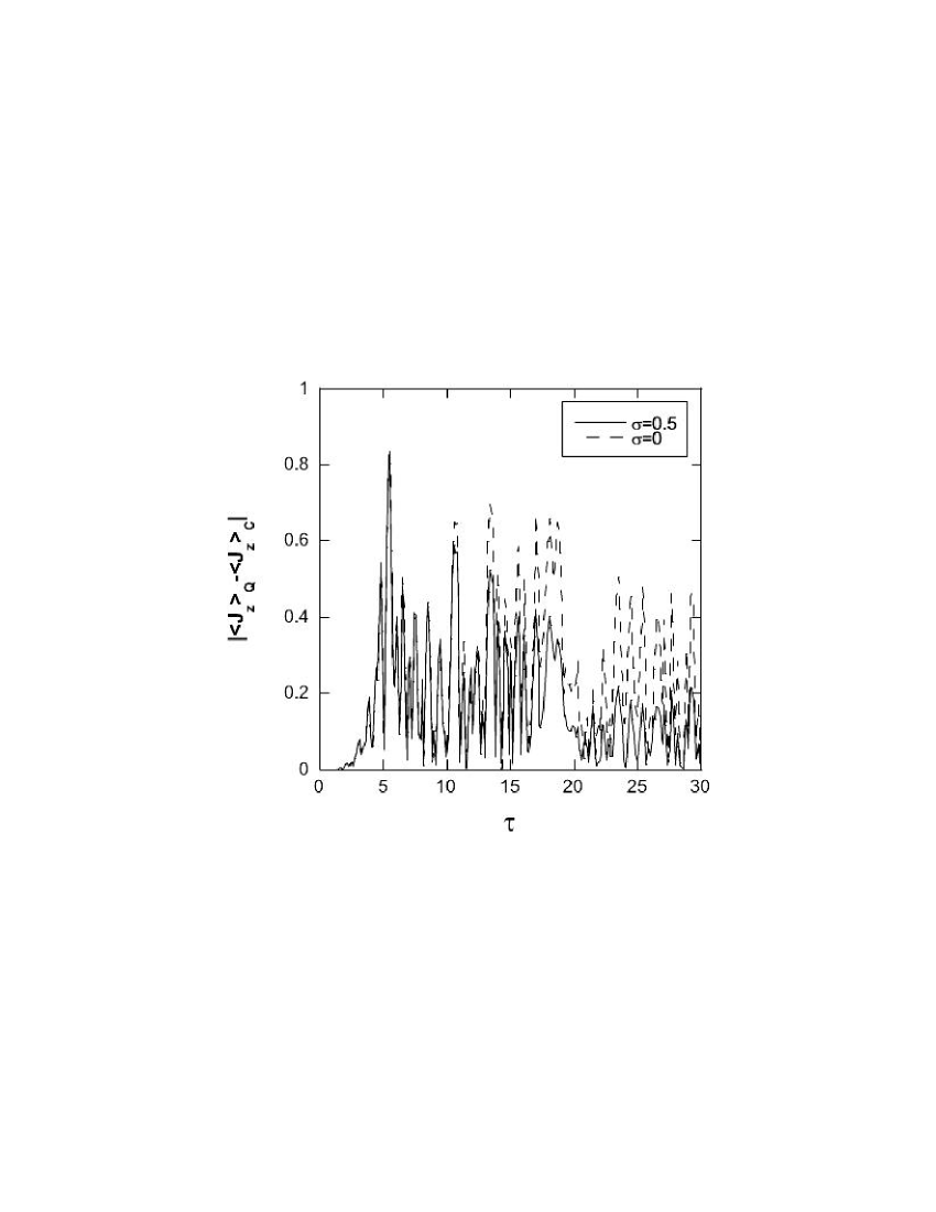
Figure 15: Variation of $\langle J_{z}\rangle$ with $\tau$ with and without the random potential with $\sigma/V_{ch}=0.024$, $\tau_{c}=0.01$. (chaotic state, $\beta=0.05$)

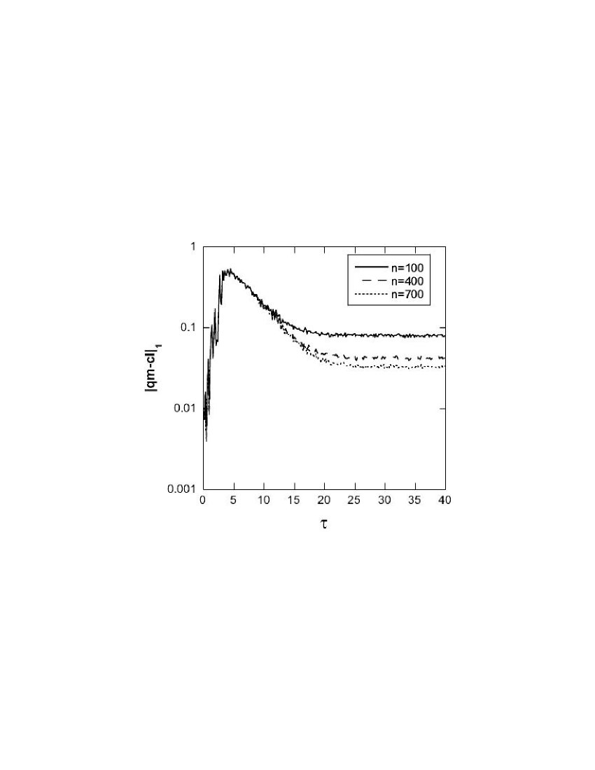
Figure 16: Variation of $|qm-cl|_{1}$ with $\tau$ for different numbers $n$ of realizations of the random potential with $\sigma/V_{ch}=0.012$, $\tau_{c}=0.01$. (chaotic state)

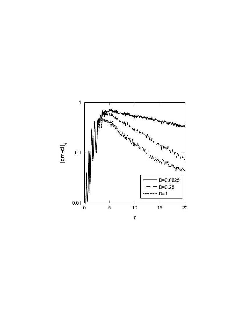
Figure 17: $|qm-cl|_{1}$ vs $\tau$ for $\beta=0.05$, for varying $D=\sigma^{2}\tau_{c}/6$.

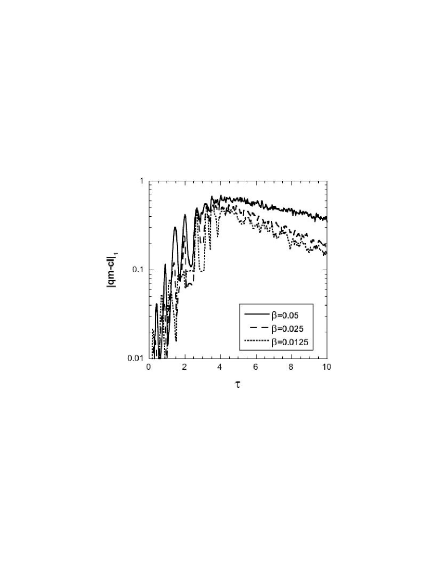
Figure 18: $|qm-cl|_{1}$ vs $\tau$ for varying $\beta$, with $\tau_{c}=0.01$ and $\sigma/V_{ch}=0.012$, for a chaotic state.

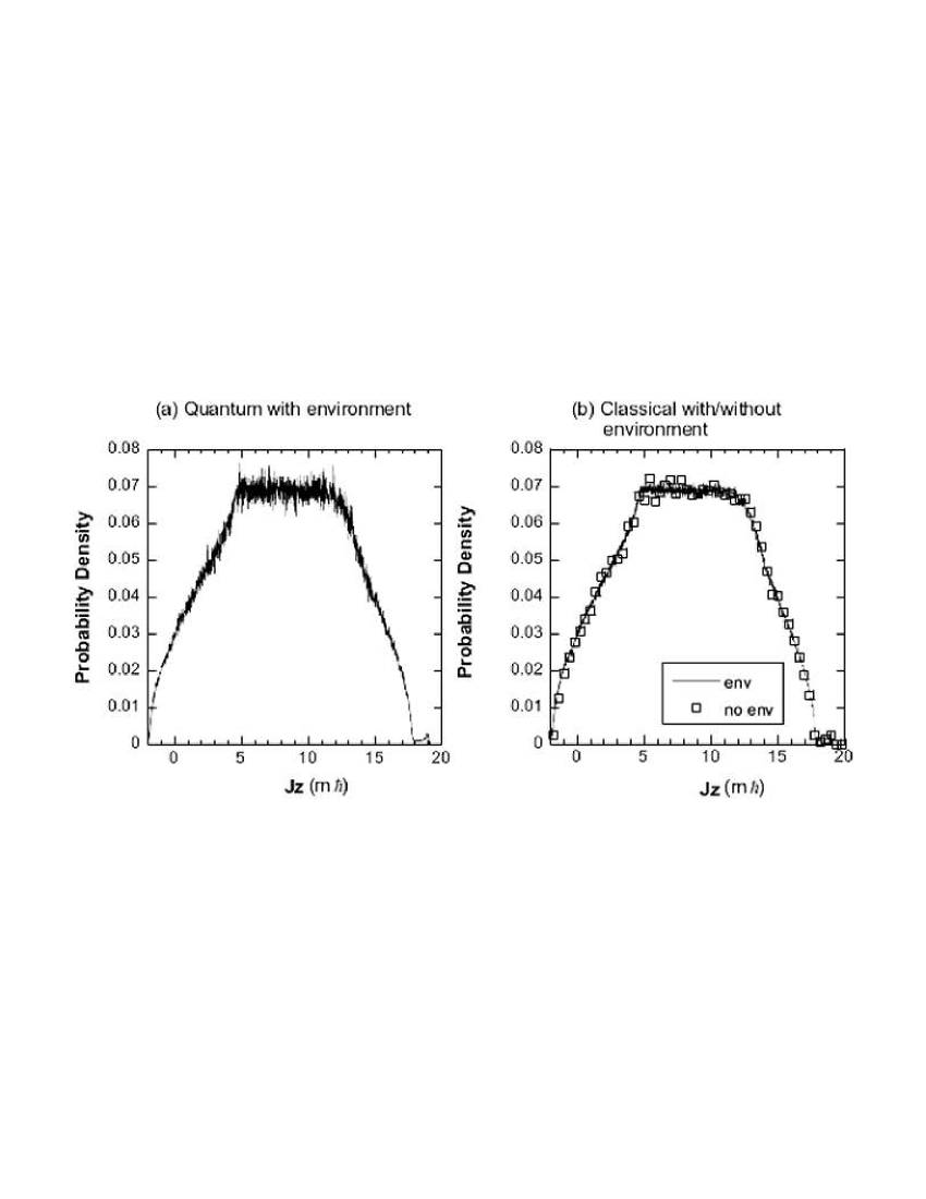
Figure 19: Quantum and Classical probability distributions at $\tau=40$, with $\beta=0.0125$, $\sigma/V_{ch}=0.012$, and $\tau_{c}=0.01$ for the chaotic state. In (b) the solid lines denote the results with the environment, and squares without the environment, showing that the classical probability distribution is not significantly affected by the environment.

Dissipation is a classical effect which results in diffusive spreading of the probability distributions. Often, the timescale for dissipation is much longer than the timescale for decoherence, and dissipation is insensitive to $\hbar$, unlike decoherence. But both effects are present together, and it is not always easy to separate them.

The effect of the environment on a quantum system is often treated by a master equation that has non-unitary time evolution. Because an initially pure state can evolve into a mixed state, it is necessary to compute the density matrix, which requires much greater storage than does the computation of a state vector. The requirements for storage and computation time scale like $K^{2}$, where K is the number of basis vectors needed to store a state vector.

An alternative method is to perform $n$ evolutions of Eq. (15) with a different realization of the random potential added for each run. Averaging the probability distributions that result from the each of the $n$ runs is physically equivalent to tracing over the environmental variables. The advantage of this method is that the computational resources for each run scale as $K$, rather than $K^{2}$ for the master equation. On the other hand, to achieve good accuracy, a large number of realizations of the random potential must be considered, in order to reduce the statistical errors in the quantum calculation. However the number of realizations of the random potential that was needed to get sufficient accuracy was considerably less than $K$, so this method was much more computationally efficient than integrating the master equation.

A stochastic potential is included, in both the quantum and classical mechanics, to model the effect of the environment on the satellite. The simplest stochastic potential that yields a random torque is

$$H_{int}=V_{0}R(t)\cos(\phi)$$ (22)

Here $R(t)$ is a correlated random function of zero mean and unit variance, $V_{0}$ is the amplitude of the random potential, and $\tau_{c}$ is its correlation time. A correlated random function is used because the fluctuations in the environment do not occur instantly, but rather they occur and decay on some time scale $\tau_{c}$. The correlated random sequence $R(t)$ can be constructed from an uncorrelated sequence, as is shown in Appendix A. The results are not sensitive to the exact form of Eq. (22), and qualitatively similar results were obtained when $\cos(\phi)$ was replaced by $\cos(2\phi)$. As is shown in Appendices B and C, the effects of the environment are expected to depend mainly on the product $\sigma^{2}\tau_{c}$, rather than on the two parameters separately. Therefore we label the results by the momentum diffusion parameter, $D=\sigma^{2}\tau_{c}/6$, which is derived in Appendix B.

The environmental perturbation should be much weaker than the tidal force on the satellite. Hence we compare the interaction potential Eq. (22) to the amplitude of the tidal potential, made dimensionless by dividing by $I_{3}/T^{2}$, which is $V_{ch}=3\sqrt{2}\pi^{2}\alpha$, or $V_{ch}\approx 21$ for $\alpha=0.5$. In all cases reported in this paper, the environmental perturbation was so weak as to have no significant effect on the classical results, so its only significant effect is to produce decoherence in the quantum results. The same parameters as in the previous chaotic case were used, $\alpha=0.5$ and $e=0.1$.

Many realizations of the random potential were computed, and the results averaged, to get an accurate measure of the effects of the environment. We used 500 realizations to obtain results that are not strongly affected by statistical errors. Fig. 15 shows the QC differences in $\langle J_{z}\rangle$, with and without the random environmental potential. The environment has no significant effect at early times, but in the saturation regime the QC differences are reduced. Since the primary effect of environmental decoherence is to destroy fine-scale structures in the probability distributions, which do not affect averages like $\langle J_{z}\rangle$, this result may seem surprising. In fact, a typical trace of $\langle J_{z}\rangle$ versus time for a single realization of the random potential will look very much like that from a run without the random potential in Fig. 15. But as time progresses, the oscillations in $\langle J_{z}\rangle$ for different realizations of the random potential tend to get out of phase with each other, and the decreased amplitudes of the QC differences in Fig. 15 are due to the averaging over the many different realizations of the random potential.

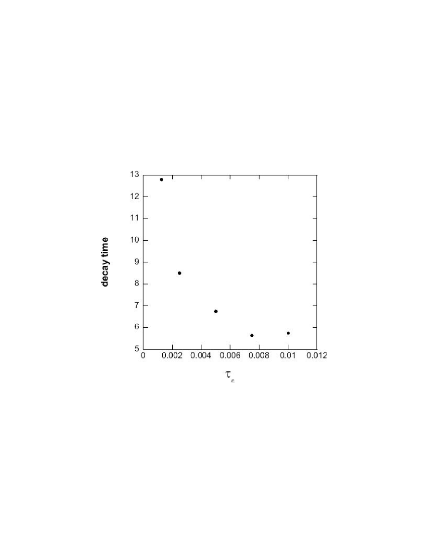
Figure 20: Decay times $\tau_{d}$ of $|qm-cl|_{1}$ vs the correlation time $\tau_{c}$ of the perturbing environment, with $\beta=0.05$, $\sigma/V_{ch}=0.012$, in the saturation regime ($\alpha=0.5$, $e=0.1$)

In Fig. 16, 100 realizations of the interaction potential were sufficient to find the maximum QC differences in $|qm-cl|_{1}$ (Eq. (19)). However, 700 realizations of the interaction potential were insufficient to resolve the QC differences in $|qm-cl|_{1}$ in the saturation regime, and so for computational reasons, these will be estimated rather than directly computed. The variation of these differences with $\beta$ and the environmental parameters can be seen in Figures. 17 and 18.

It can be seen in Fig. 19 that, with the inclusion of the environmental perturbation, the quantum probability distribution is much closer to the classical distribution than without the environment (compare Fig. 12).

V.1 Environmental Effects in the Saturation Regime

In the saturation regime, the QC differences in $|qm-cl|_{1}$ (Eq. (19)) appear to decay exponentially from their maximum value to a saturation level (see Fig. 17 and 18). The rate of this decay is a duffusion time, and is not the decoherence time, as will be shown shortly. From Fig. 20 it is clear that, for sufficiently large values of $\tau_{c}$, the decay time $\tau_{d}$ no longer depends on $\tau_{c}$, but settles at $\tau_{d}\approx 5.6$. For sufficiently large $\sigma$ and sufficiently small $\beta$, the decay time was found to also have approximately this same limit.

To test whether this decay rate is governed by quantum mechanics, we compared two classical ensembles with different initial values of $J_{0}$ ($J_{0}=10$ and $J_{0}=11$), and computed the 1-norm of the difference between them as a function of time. Fig. 21 shows that these initially different classical ensembles converge at a rate given by $\tau_{d}=5.6$. So, apparently, this time scale measures how quickly the differences between two different distributions decrease as they both grow to fill the chaotic sea.

It is not clear from Fig. 17 and 18 whether the QC differences in the probability distributions eventually decrease to zero or reach a non-zero long-time limit. In Fig. 22 the long-time saturation level of $|qm-cl|_{1}$ is plotted as a function of the number $n$ of realizations of the random potential. In the limit $n\rightarrow\infty$ the QC differences approach a small value that appears to be slightly positive. However that extrapolated limit is substantially smaller than the typical statistical errors for ensemble sizes of 1,000,000 to 2,000,000, and so is not significantly different from zero.

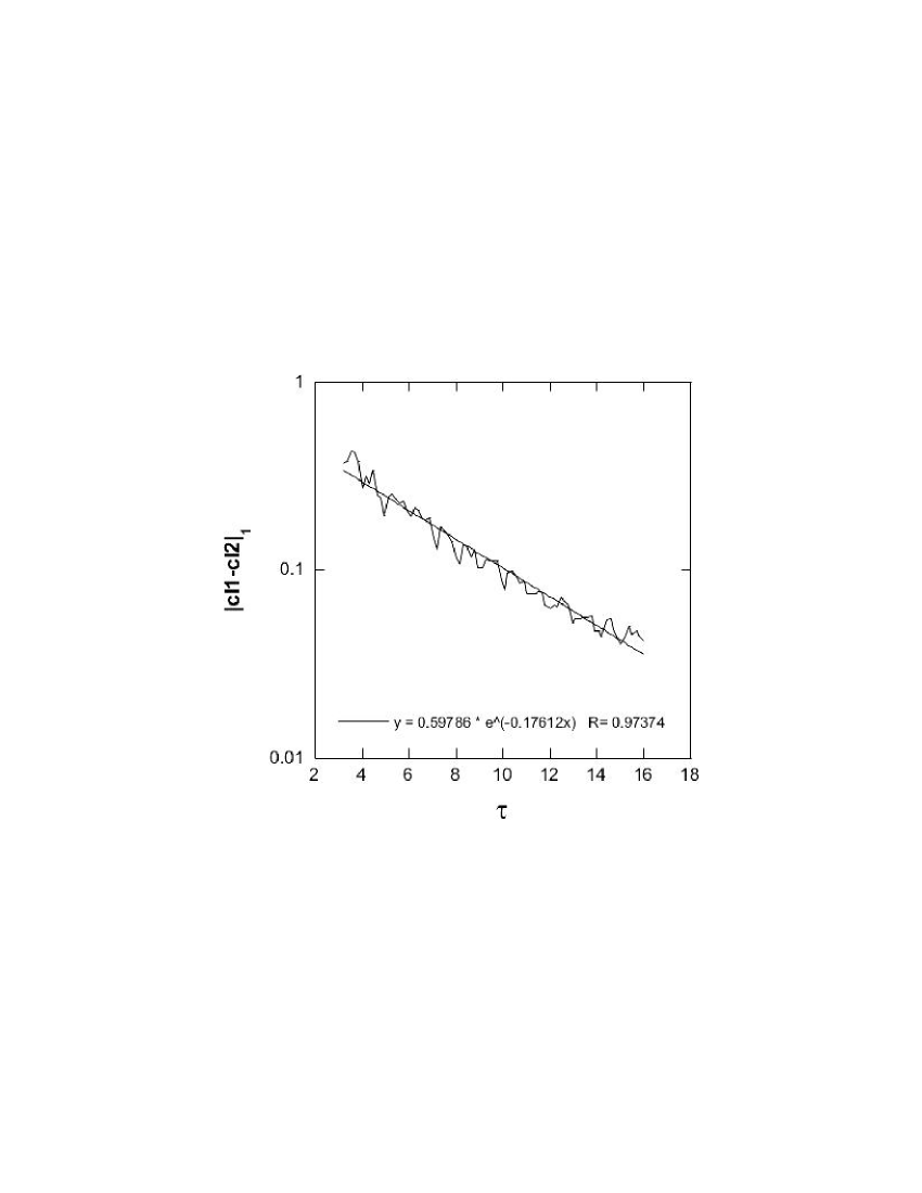
Figure 21: 1-norm of the difference between two classical ensembles, one with $\langle J_{z}\rangle=10$, the other $\langle J_{z}\rangle=11$. $\beta=0.05$, $\sigma/V_{ch}=0.012$, $\tau_{c}=0.01$

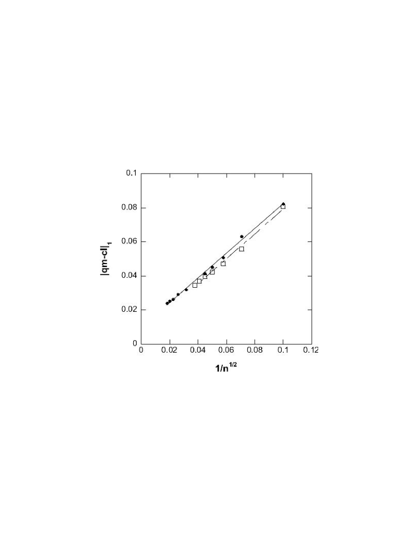
Figure 22: $|qm-cl|_{1}$ vs $n^{-1/2}$ at $\tau=40$. $n$ is the number of realizations of the random potential. ($\sigma/V_{ch}=0.012$, $\tau_{c}=0.01$ for the chaotic state)

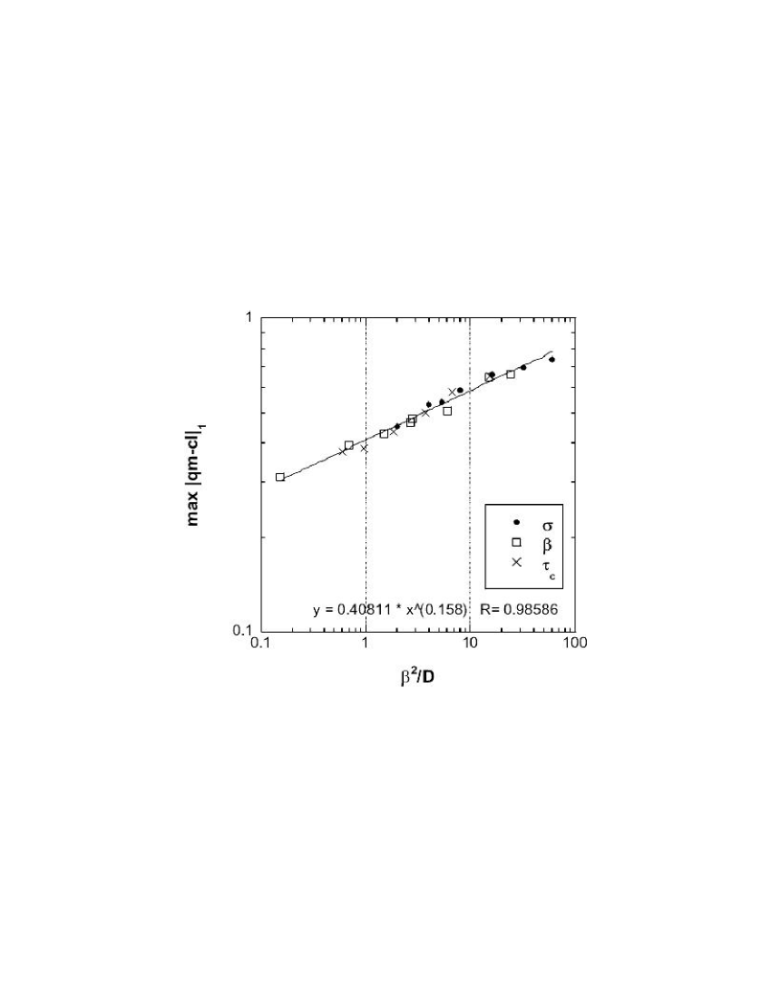
Figure 23: Maximum values of $|qm-cl|_{1}$ vs $\beta^{2}/D$. The points labeled $\beta,\sigma,and\tau_{c}$ represent data sets where $\beta,\sigma,$ and $\tau_{c}$ were varied with the other two parameters held constant.

V.2 Scaling of the Maximum QC Differences

The maximum value of $|qm-cl|_{1}$ for the quantum and classical probability distributions must depend on the three parameters $\beta$, $\sigma$, and $\tau_{c}$. However, in agreement with arguments presented by Pattanayak et al. Pattanayak et al. (2003), the data was found to collapse onto a single curve parameterized by $\xi=\beta^{2}/D$ (Fig. 23). From a least squares fit, the scaling relationship was found to be

$$\max(|qm-cl|_{1})\propto\left(\frac{\beta^{2}}{D}\right)^{\frac{1}{6}}$$ (23)

This scaling as $\hbar^{1/3}$ was also found for a coupled rotor model without decoherence Ballentine (2004). This result suggests that the $\beta^{1/3}$ scaling found here might be generic for systems with more than one degree of freedom, and also suggests that the pointwise convergence of the quantum probability distribution to the classical distribution may occur because of other interacting degrees of freedom (not necessarily an external environment).

V.3 Effects of Decoherence vs Smoothing

The effect of environmental decoherence is analogous to applying a smoothing filter to the quantum distributions, but the two effects are not exactly the same. A small amount of smoothing does not affect the average values of an observable, whereas decoherence can have an effect by dephasing the quantum fluctuation, which are then averaged over (see Fig. 15). This effect may be peculiar to systems with only one degree of freedom.

Another difference is in the scaling of the QC differences with the parameters. Figure 24 shows $|qm-cl|_{1}$ in the saturation regime as a function of $\beta$ and $\Delta_{s}$, where $\Delta_{s}$ is the half width of the triangular filter used to smooth the quantum distribution. In the saturation regime, $|qm-cl|_{1}$ was found to depend on the single parameter $\beta/\Delta_{s}$, where it obeys the scaling relation

$$|qm-cl|_{1}=0.58\left(\frac{\beta}{\Delta_{s}}\right)^{0.44}$$ (24)

Eq. (24) shows a scaling relationship similar to Eq. (23). This may be understood as follows. Environmental perturbations cause momentum diffusion. This effect is proportional to $\sqrt{D}$, and so $\Delta_{s}$ should be compared to $D^{2}$. Hence, in the late time limit, smoothing and decoherence rely on a similar composite parameter. However the power laws are different in the two cases, and so the two processes are not entirely equivalent.

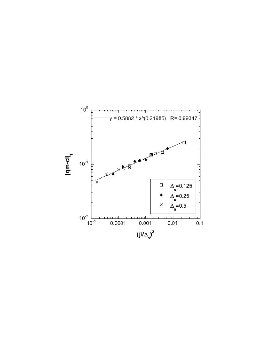
Figure 24: $|qm-cl|_{1}$ for smoothed probability distributions for varying $\sigma_{m}$ and $\beta$ in the saturation regime ($\tau=20$).

In summary, the environmental perturbations were found to drasticly reduce the fine-scale structure in the quantum distributions. The measure of the QC differences, $|qm-cl|_{1}$ , was found to initially increase with $\tau$ in a form similar to the results in Sec. IV. After reaching a maximum value, $|qm-cl|_{1}$ then decreased exponentially with time. The decay time was found to be a classical diffusion time, and not a decoherence time. The maximum QC differences were found to scale as $(\beta^{2}/D)^{1/6}$, where $D$ is the momentum diffusion parameter.

VI Classical Limit for Hyperion

VI.1 QC Differences Without Environment

Having calculated the QC differences for the chaotic rotation of a tidally driven satellite, and determined how they scale with the relevant parameters, we shall now use this information to estimate the magnitude of quantum effects on Hyperion. In particular, we shall assess Zurek’s claim Zurek and Paz ; Zurek (1998) that environmental decoherence is needed to ensure its classical behavior. We first examine the magnitude of the QC differences for Hyperion if the effect of the environment is ignored.

First we must determine the dimensionless parameter $\beta=\frac{\hbar T}{I_{3}}$. Using Hyperion’s mean density of $\rho=$ 1.4 g cm^-3, and treating it as an ellipsoid with moments of inertia $I_{3}>I_{2}>I_{1}$, then $I_{3}=2.1\times 10^{29}$ kg m². Using the value of $\hbar=1.05\times 10^{-34}$ J s, and the orbital period $T=1.8\times 10^{6}$ s, then yields

$$\beta=9.3\times 10^{-58}$$ (25)

In Sec. IV B it was found that the maximum QC differences in $\langle J_{z}\rangle$ scale as $\beta^{2/3}$. Hence the maximum QC difference in the dimensionless angular momentum $\langle J_{z}\rangle$ for Hyperion should be approximately $5\times 10^{-37}$. So there should be no observable difference between the quantum and classical averages of angular momentum for Hyperion.

This result contradicts Zurek’s claim that, if decoherence is ignored, there should be a break time of no more than 20 years, beyond which the QC differences would become macroscopic. As was pointed out in the Introduction, if that break time is interpreted as the limit of the Ehrenfest regime, then it does not mark the end of the classical domain. But in Zurek and Paz a break time of a similar order of magnitude was estimated for the end of the Liouville regime. Both of those estimates were based on an exponential growth of the QC differences that occur in a chaotic state. Now the deviations from Ehrenfest’s theorem do, indeed, grow exponentially until they reach the size of the system, as is needed for Zurek’s argument to succeed. But, as was shown in Sec. IV(A), the exponential growth of the differences between quantum state averages and classical ensemble averages will saturate before those differences reach the size of the system, and the saturation value scales with a small power of $\hbar$. Hence, for the actual (small) value of $\hbar$, the QC differences in the Liouville regime can remain small for all time, and there is no effective break time for the regime of classicality.

The differences in $\langle J_{z}\rangle$ become vanishingly small in the classical limit, but this does not imply that the full quantum probability distribution converges to the classical limit. We know that the quantum probability distribution will not converge to the classical distribution in a pointwise fashion. But we can ask what resolution is needed for a detector to be able to discriminate between these two distributions. Let us suppose that two probability distributions are practically indistinguishable when $|qm-cl|_{1}<0.01$. Using scaling result in Fig. 24, we find that a resolution $\Delta_{s}$ of 1 part in $10^{-60}$ rad/s is needed to resolve the two probability distributions. This suggests that it would be practically impossible to observe the quantum effects in the probability distributions, even without invoking environmental decoherence.

VI.2 Environmental Effects on Hyperion

There are many environmental perturbations that can affect the satellite: random motion of the particles within the satellite, random collisions with interplanetary dust, and random light fluctuations from the sun, to name a few. We shall consider the random collisions with dust particles as an example.

To do this we treat the interplanetary dust as a dilute gas, and Hyperion as a sphere rotating about a fixed axis under the influence of random motion of the fluid. The dimensional momentum diffusion parameter is Coffey et al. (2004)

$$\tilde{D}=16\pi k\mathcal{T}R_{h}^{3}\eta$$ (26)

Using Eq. (40), the dimensionless momentum diffusion parameter D is

$$D=\frac{8\pi k\mathcal{T}R_{h}^{3}\eta T^{3}}{I_{3}^{2}}$$ (27)

Here $T$ is the temperature, $k$ is Boltzmann’s constant, $R_{h}$ is the radius of Hyperion, and $\eta$ is the kinetic viscosity of the dust fluid, which, following Present (1958), is calculated to be

$$\eta=\frac{nm\bar{v}L}{3\sqrt{2}}$$ (28)

Here $\bar{v}$ is the rms velocity of the dust particles, $m$ is their mass, $n$ is their number density, and $L=1/{n\pi r^{2}}$ is their mean-free-path, and $r$ is the radius of a dust particle.

The properties of interplanetary dust were measured by the Voyager space probes. The average number density of particles near Saturn is $n=4\times 10^{-8}$ m^-3 Gurnett et al. (2002). The average mass of the dust grains is estimated to be $m=10^{-10}$ g, and their radius is about $r=10^{-6}$ m. The temperature in the vicinity of Saturn is about $\mathcal{T}\approx$ 135 K Caroll and Ostlie (1996).

Using Eq. (28), treating Hyperion as a sphere of radius $R_{h}=150$ km, and using $\eta=1.8\times 10^{-6}$ Pa s for the kinetic viscosity, we estimate the dimensionless angular momentum diffusion parameter to be $D\approx 6.4\times 10^{-50}$. Even such a small value is sufficient to reduce $|qm-cl|_{1}$ substantially. Using Eq. (23), the order of magnitude of $|qm-cl|_{1}$ for Hyperion is found to be $10^{-10}$. This implies that the classical and quantum probability distributions will agree almost exactly for a large body such as Hyperion. Without the influence of the environment, the value of $|qm-cl|_{1}$ due to the very fine-scale differences between the quantum and classical probability distributions might be of order unity. But, of course, these differences would be impossible to resolve because they exist on such a very fine scale. So the effect of decoherence is to destroy a fine structure that would be unobservable anyhow.

VII Conclusion

In this paper the regular and chaotic dynamics of a satellite rotating under the influence of tidal forces was examined, with application to the motion of Hyperion. Quantum and classical mechanics were compared for both types of initial state, and the scaling with $\hbar$ of the quantum-classical (QC) differences was determined. The effect of the environment was modeled, and its effect on the QC differences was estimated, so as to determine whether environmental decoherence is needed to account for the classical behavior of a macroscopic object like Hyperion. Two measures of the differences between quantum and classical mechanics were examined: the QC difference in the average angular momentum, $|\langle J_{z}\rangle_{Q}-\langle J_{z}\rangle_{C}|$, and the differences between the probability distributions, $|qm-cl|_{1}$ (Eq. (19)).

For early times, the QC differences in $\langle J_{z}\rangle$ grow in time as $\tau^{2}$ for the non-chaotic state, and as $e^{2.9\tau}$ for the chaotic state. At longer times, the QC differences saturate for the chaotic state, but oscillate quasi-periodically for the non-chaotic state. The magnitude of the QC differences scale as $\beta^{2}$ (dimensionless $\hbar$) at early times, for both the chaotic and non-chaotic states. This $\beta^{2}$ scaling persists for all times for the non-chaotic state. But the QC differences that occurs in the saturation regime of the chaotic state scale as $\beta^{2/3}$. A similar scaling has also been observed for a model of two coupled rotors Ballentine (2004), so this result is not peculiar to the particular model studied in this paper.

The value of the dimensionless $\hbar$ for Hyperion is $\beta=9.3\times 10^{-54}$, for which the $\beta^{2/3}$ scaling relation predicts a maximum value for the QC difference in $\langle J_{z}\rangle$ to be $5\times 10^{-37}$. Therefore, there is no need to invoke environmental decoherence to explain the classical behavior of $\langle J_{z}\rangle$ for a macroscopic object like Hyperion.

Although the differences between the quantum and classical averages of observables becomes very small in the macroscopic limit, this need not be true for the differences between quantum and classical probability distributions. Indeed, the quantum probability distributions do not converge pointwise to the classical probability distributions, for either the non-chaotic or the chaotic states. A modest amount of smoothing of the quantum distribution reveals that it is made up of an extremely fine-scale oscillation superimposed upon a smooth background, and its is that smooth background that converges to the classical distribution. Similar behavior has been found for other one-dimensional systems Ballentine (1999). This smoothing can be regarded as an inevitable consequence of the finite resolving power of the measuring apparatus. Alternatively, it may be impossible to observe the fine structure because of environmental decoherence. At the macroscopic scale of Hyperion, the primary effect of decoherence is to destroy a fine structure that is anyhow much finer than could ever be resolved by measurement.

When the environment was included, the results were found to follow a scaling relationship proposed by Pattanayak et al. (2003): the maximum distance between the classical and the quantum probability distributions is proportional to $(\beta^{2}/D)^{1/6}$. Here $D$ is the momentum diffusion parameter (see Appendix B). This suggests that the quantum probability distributions will approach the classical distributions pointwise as $\beta\rightarrow 0$, provided that $D$ is non-zero. With environmental perturbations included, the QC differences in the probability distributions scaled as $|qm-cl|_{1}\propto\beta^{1/3}$. A similar scaling was also found for two autonomous coupled rotors Ballentine (2004). This suggests that pointwise convergence of the quantum probability distribution to the classical value may be typical for systems with more than one degree of freedom, and the lack of such convergence for systems with only one degree of freedom may be pathological. The role of the environment, in the model of this paper, is then to cure this pathology by supplying more degrees of freedom.

Taking $D$ to be the momentum diffusion parameter for rotation of Hyperion due to collisions with the interplanetary dust around Saturn, we find (estimated from Eq. (23)) that the maximum of $|qm-cl|_{1}$ that Hyperion should exhibit should be of order $10^{-10}$. Thus decoherence would cause the quantum probability distribution to converge to the classical distribution in essentially a pointwise fashion.

Coarse graining (due to the finite resolution power of the measurement apparatus) will also decrease the QC differences in the probability distributions. In the saturation regime, the measure $|qm-cl|_{1}$ of that difference was found to be proportional to $(\beta/\Delta_{s})^{0.44}$, where $\Delta_{s}$ is the width of the smoothing filter. This shows that decoherence and smoothing have similar effects. But they are not exactly equivalent, since their effects scale with somewhat different values of $\beta$.

In conclusion, we find that, for all practical purposes, the quantum theory of the chaotic tumbling motion of Hyperion will agree with the classical theory, even without taking account of the effect of the environment. Decoherence aids in reducing the quantum-classical differences, but it is not correct to assert that environmental decoherence is the root cause of the appearance of the classical world.

Appendix A Correlated Random Number Generation

To describe the effect of environmental perturbations, we require a sequence of correlated random numbers. Generators for uncorrelated random variates are commonly available, but algorithms for generating a correlated sequence are not common. We show here how to generate a random sequence having a controlled amount of correlation from a standard sequence of independently distributed random numbers. Let $\{r_{i}\}$ be such a sequence, with zero mean and unit variance.

$$\langle r_{i}\rangle=0$$ (29)

$$\langle r_{i}r_{j}\rangle=\delta_{ij}$$ (30)

To generate a correlated sequence $\{R_{i}\}$ from the uncorrelated sequence, we simply form linear combinations,

$$R_{i+1}=cR_{i}+(1-c)r_{i+1}$$ (31)

where $c$ is a chosen positive constant $(c<1)$, and $R_{1}\equiv r_{1}$. It follows from Eq. (31) that

$$R_{i+1}=c^{i-1}r_{1}+\sum_{m=0}^{i-1}c^{m}(1-c)r_{i+1-m}$$ (32)

From this result, we can calculate the degree of correlation in our new sequence. Taking $i>j$, and using Eq. (32) and Eq. (30), we obtain

$$\langle R_{i}R_{j}\rangle=\sum_{m=0}^{i-2}\sum_{m^{\prime}=0}^{j-2}c^{m+m^{\prime}}(1-c)^{2}\langle r_{i+1-m}r_{j+1-m^{\prime}}\rangle+$$

$$\sum_{m=0}^{i-2}c^{m}(1-c)c^{j-1}\langle r_{1}r_{i+1-m}\rangle+$$

$$\sum_{m^{\prime}=0}^{j-2}c^{m^{\prime}}(1-c)c^{i-1}\langle r_{j+1-m^{\prime}}r_{1}\rangle+c^{i-j-2}\langle r_{1}^{2}\rangle$$

Eq. (A) can be simplified using Eq. (30). Performing the resulting geometric sums then yields

$$\langle R_{i}R_{j}\rangle=\left(\frac{1-c}{1+c}\right)c^{i-1}(c^{1-j}-c^{j-1})$$ (34)

For $j\gg 1$ and $c<1$, Eq. (34) becomes:

$$\langle R_{i}R_{j}\rangle\approx\left(\frac{1-c}{1+c}\right)c^{i-j}$$ (35)

This discrete sequence must now be converted into a function of time. Each $R_{i}$ refers to the correlated random function at time $t_{i}$. Taking the time interval between the random numbers to be $\Delta t$, then it is appropriate to define a correlation time $\tau_{c}=\Delta t/|\ln(c)|$ for the correlated random function, for which we have

$$\langle R(0)R(\tau)\rangle\approx\left(\frac{1-c}{1+c}\right)e^{-\tau/\tau_{c}}$$ (36)

Appendix B Momentum Diffusion Parameter

The momentum diffusion parameter ($D$) is needed to calculate the effect of the environment on the system Unruh and Zurek (1989); Anglin et al. (1997); Strunz et al. (2003). In particular, the form of $D$ is needed to show that the scaling result in Pattanayak et al. (2003) applies also to our model.

Consider the random potential of the form $V=V_{0}\cos(\phi)$. The random torque is then $F=V_{0}R(t)\sin(\phi)$. Here $R(t)$ is a correlated random function, as defined in Appendix A. From this, we can find the momentum diffusion parameter through the relation

$$\tilde{D}=\lim_{t\rightarrow 0}\frac{\langle s(t)^{2}\rangle}{t}$$ (37)

The integral of the torque over time yield the angular momentum, hence the variance of the angular momentum under this random torque is given by

$$\langle s^{2}(t)\rangle=\frac{V_{0}^{2}}{2}\int_{0}^{t}\!\int_{0}^{t}dt^{\prime}\,dt^{\prime\prime}\,\langle R(t^{\prime})R(t^{\prime\prime})\rangle$$

$$=\frac{V_{0}^{2}}{2}\int_{0}^{t}\!\int_{0}^{t}dt^{\prime}\,dt^{\prime\prime}\,\left(\frac{1-c}{1+c}\right)c^{|t^{\prime}-t^{\prime\prime}|/t_{c}}$$

$$=V_{0}^{2}\left(\frac{1-c}{1+c}\right)(t_{c}^{2}+t_{c}t+t_{c}^{2}\exp(-t/t_{c}))$$ (38)

The quantity $s(t)$ is the standard deviation of the angular momentum for a random walk under the influence of Eq. (22), and $\sigma$ is the standard deviation of the random potential. For $t\gg t_{c}$ we have

$$\langle s^{2}(t)\rangle\approx tt_{c}V_{0}^{2}\left(\frac{1-c}{1+c}\right)$$ (39)

Using 37 and choosing the value $c=1/2$, we obtain momentum diffusion constant $\tilde{D}$ to be

$$\tilde{D}=\frac{V_{0}^{2}t_{c}}{3}$$ (40)

In the body of this paper, we use a dimensionless momentum diffusion parameter D. The relation between these two quantities is

$$D=\tilde{D}\frac{T^{3}}{2I_{3}^{2}}=\frac{\sigma^{2}\tau_{c}}{6}$$ (41)

where $\tau_{c}$ is defined to be $\tau_{c}=t_{c}/T$, and $\sigma=V_{0}T^{2}/I_{3}$.

Appendix C Derivation of Scaling Parameter

Pattanayak et al. Pattanayak et al. (2003) suggested that at long times the QC differences in the probability distribution should become a function of the single parameter $\xi$, where $\xi=\hbar^{a}\lambda^{b}D^{c}$, for some powers $a$, $b$ and $c$. Here $D$ is the diffusion parameter, defined in Appendix B, and $\lambda$ is the classical Lyapunov exponent.

The argument is similar to one presented in Zurek (1998). It assumes that the differences between quantum and classical mechanics are due to the Moyal terms in the equation of motion for the Wigner function. These terms have the form

$$\sum_{n=1}^{\infty}\frac{\hbar^{2n}}{2^{2n}(2n+1)!}\partial_{\phi}^{2n+1}V(\phi)\partial^{2n+1}_{p}\rho^{w}$$ (42)

where $\rho^{w}$ is the Wigner function for the state. For a chaotic system, the phase space distribution will develop very fine structures as it fills the accessible phase space, with the rate at which these fine structures develop being governed by the Lyapunov exponent $\lambda$. Since these terms depend on $\partial^{2n+1}_{p}\rho^{w}$, they will become larger as time progresses and the fine structure grows. However the inclusion of environmental perturbations on system causes diffusion, which will limit the growth of the fine structure. When these effects balance each other, the fine structure is expected to have an equilibrium scale Pattanayak et al. (2003); Zurek (1998) given by

$$\frac{\partial\rho^{w}}{\partial p}\approx\sqrt{\frac{\lambda}{2D}}$$ (43)

If this equilibrium momentum scale is sufficiently large compared to $\hbar$, then only the first order Moyal term should be significant. Under this assumption, the QC differences should be a function of this Moyal term, given by

$$\xi=\hbar^{2}\lambda^{5/2}D^{-(3/2)}\frac{\partial^{3}V(\phi)}{\partial\phi^{3}}$$ (44)

It is argued Zurek (1998) that the characteristic scale on which $\rho^{w}$ varies is $\delta\phi\propto\sqrt{D/\lambda}$. The characteristic variation of $\partial^{3}_{\phi}V(\phi)$ can be found by a Taylor expansion of $\partial^{3}_{\phi}V(\phi)\propto\sin(\phi)$ about an arbitrary point $\phi_{0}=0$. Averaging the result over $\phi_{0}=0$ then yields

$$\frac{\partial^{3}V(\phi)}{\partial\phi^{3}}\propto\delta\phi\approx\sqrt{\frac{D}{\lambda}}$$ (45)

Inserting Eq. (45) into Eq. (44) yields

$$\xi\propto\frac{\hbar^{2}}{D}$$ (46)

Thus, once the growth fine scale structure of the probability distribution reaches equilibrium with diffusion, the QC differences in the probability distribution should be a function of $\hbar^{2}D^{-1}$. The results in Sec. V confirm this conclusion.