The dissertation of Eric Dennis is approved.

————————————————————————
Herschel Rabitz (Princeton University)

————————————————————————
David Awschalom

————————————————————————
Matthew Fisher

————————————————————————
Philip Pincus

————————————————————————
Atac Imamoglu, Committee chair

July 2003

© September 2024

All Rights Reserved

Acknowledgements

I would like to thank my advisors Atac Imamoglu and Hersch Rabitz for their guidance and instruction, David Awschalom for giving me the opportunity to see what a qubit really looks like, John Preskill for his methodical lessons in quantum information, and the grad students and post-docs who have helped and entertained me along the way, in particular Mike Werner, Ignacio Sola, Jay Kikkawa, Jay Gupta, Dan Fuchs, Andrew Landahl, Dave Beckman, and Daniel Gottesman. I am also grateful to Nino Zanghi, Sheldon Goldstein, and Roderich Tumulka for their intransigence, and to Travis Norsen for his level-headedness. I have been supported by the Army Research Office, the Princeton Plasma Physics Laboratory, and the National Science Foundation.

Vita
Eric Dennis

Education

Bachelor of Science (honors), California Institute of Technology, June 1998.
Master of Science in Physics, UC Santa Barbara, Sept. 2000.
Doctor of Philosophy in Physics, UC Santa Barbara, Sept. 2003 (expected).

Professional Employment

Summers 1994-98: Research Assitant, California Institute of Technology.
1998-2000: Research Assistant, Dept. of Physics, UC Santa Barbara.
2000-03: Research Assistant, Dept. of Chemistry, Princeton University.

Publications

E. Dennis, “Toward fault-tolerant computation without concatenation,” Phys. Rev. A 63 052314 (2001); presented as an invited talk at 1999 SQuINT annual conference.
E. Dennis, A. Kitaev, A. Landahl, J. Preskill, “Topological quantum memory,” J. Math. Phys. 43 4452 (2002).
E. Dennis, H. Rabitz, “Path integrals, stochastic trajectories, and hidden variables,” Phys. Rev. A 67 033401 (2003); presented as an invited talk at CECAM workshop in Lyon, France (Sept. 2002).

Awards

Three PPST Fellowships, Princeton Plasma Physics Laboratory (6/01–6/03).

Fields of Study

Major Field: Quantum Information
Study in Quantum Error Correction with Prof. Atac Imamoglu.
Study in Experimental Condensed Matter Physics with Prof. David Awschalom.
Study in Quantum Control and Simulation with Prof. Herschel Rabitz.

The problems of decoherence and destructive measurement make quantum computers especially unstable to errors. We begin by exploring Kitaev’s framework for quantum error correcting codes that exploit the inherent stability of certain topological quantum numbers. Analytic estimates and numerical simulation allow us to quantitatively assess the conditions under which this stability persists. In order to allow quantum computations to be performed on data stored in these and other unconcatenated codes, we present a probabilistic algorithm for executing an encoded Toffoli gate via preparation of a certain three-qubit entangled state as a computational resource. The algorithm works to iteratively purify an initial input state, conditional on favorable measurement outcomes at each stage in the iteration.

Analogous iterative purification methods are identified in the context of classical algorithms for simulating quantum dynamics. Here an ensemble of stochastic trajectories over a classical configuration space is iteratively driven toward a fixed point that yields information about a quantum evolution in an associated Hilbert space. We test this procedure for a restricted subspace of the Heisenberg ferromagnet.

The trajectory ensemble concept is then applied to the problem of mechanism identification in closed-loop quantum control, where a precise definition of mechanism in terms of these trajectories leads to methods for extracting dynamical information directly from the kinds of optimization procedures already realized in control experiments on optical-molecular systems. We demonstrate this on simulated data for controlled population transfer in a seven level molecular system under shaped-pulse laser excitation.

Chapter 1 Elements of Quantum Information

1.1 Universal Quantum Simulators

It is a bromide among particle physicists that the standard model contains (or that some still undefined string/M theory may someday contain) all the rest of physics at lower energy scales and that the problem is just the difficulty of actually computing its implications on these scales. It is a bromide among condensed matter physicists that chemistry and materials science are likewise reducible to one large $N$-particle Schrodinger equation. And it is a bromide among chemists that biology is reducible in some such way to chemistry.

But why are even the most sophisticated modern computers unable to seriously penetrate these age-old disciplinary boundaries? It appears that the main obstacle to exploiting this reductionism is native to quantum mechanics, and it is not so subtle. Consider how a computer could represent a purely classical, physical system. Assuming a discretized state space so that for $N$ distinguishable particles each may occupy one of $S$ possible states, the total amount of information necessary for a computer to store one particular configuration of the system is just $N\log_{2}S$ bits. One particular state of the corresponding quantum system, however, will require for its description a set of $S^{N}$ complex numbers, one for every possible classical state. This means the number of bits necessary for a computer to store this description will grow exponentially, not linearly, with $N$. As $N$ gets large, not only does it become computationally intractable to predict the future behavior of the system—it is intractable even to fully specify its present state.

Something here is not quite right, though. The desired result of a given quantum simulation may not necessarily include a complete quantum description of some final state. The heat capacity of a metal for instance—while requiring a quantum mechanical treatment in certain circumstances—is still just one number. It is only the intermediate stages in the calculation which presumably require consideration of these intractable quantum state vectors. But perhaps there are alternative representations which obviate such huge memory sinks. Indeed there are, and they succeed in eliminating the exponential blow-up of storage and computation costs for certain kinds of systems. However, no such techniques exist that work on a more general level, and their effectiveness at particular problems is something of an open question to be probed one problem at a time.

This leads to a more pessimistic appraisal: if ab initio computation is in general so expensive, why bother with it at all? If one is interested in the behavior of a generic quantum system in the laboratory, perhaps it will always be easier to perform actual experiments on the system itself. Let the system perform the computations for you! Indeed the physical system may be regarded as a kind of ultra-special purpose computer, fit for exactly one problem. Perhaps one is more ambitious, however, and might attempt to use one physical system that is especially accessible in the laboratory in order to simulate some other kind of system entirely. For instance there are proposals to study gravitational systems by resort to analogies in condensed matter [1], whereby the material relations for certain liquids are seen to fortuitously mimic some aspects of the Einstein field equations.

Even bolder would be to imagine that certain quantum systems, by virtue of some special types of interactions, are able to simulate large classes of quantum systems in a way which is less fortuitous and more by design. In essence, exactly this is what is going on in a classical computer when it simulates other classical systems. There is no real physical similarity between a silicon microchip and the turbulent flow of nitrogen gas which it simulates via a fluid dynamics algorithm. Why can’t such a computational universality exist in the quantum domain as well?

This was the motivation of Feynman when he proposed the idea of a quantum computer as a universal quantum simulator [2].

A sufficiently well controlled quantum mechanical system that can be initialized in a chosen state, evolved by tunable interactions, and measured with high fidelity deserves the title quantum computer if these interactions are sufficiently universal as to mimic a large class of other quantum systems bearing little physical relationship to that of the computer. The crux of quantum computation is in this notion of computational universality. The difference between a liquid Helium system mimicking the quantum fluctuations of space-time and a quantum computer mimicking, say, the molecular dynamics of water is that tomorrow the quantum computer may be used to simulate something entirely different; whereas, the liquid Helium system will always be stuck on the same physical problem of quantum gravity.

As opposed to the Helium system, which achieves its mimickery through a kind of mathematical coincidence, the quantum computer works (rather, would work, if ever one were built) by detailed independent control of many many individualized components. The basic unit of the quantum computer is the quantum bit (or qubit). One qubit is a quantum system represented by a two-dimensional Hilbert space with basis states conventionally denoted as $|0\rangle$ and $|1\rangle$. $N$ qubits are represented by the space spanned by all states $|x\rangle$ where $x$ is an $N$-bit binary string. The dimension of this space thus grows as $2^{N}$.

A general quantum system with classical configuration space $Q$ may then be represented as an $N$-qubit system by discretizing $Q$ into $2^{N}$ elements. In order to simulate the system evolution in the quantum computer, this evolution must be discretized in time, and each resulting unitary step must be translated into operations to be performed on the qubits. In particular if the classical configuration space $Q=(0,1)^{\otimes N}$ for $N$ distinguishable particles in 1d is discretized such that the $i$-th coordinate can be represented by a bit string $x_{i}$ (containing, say, $S$ bits), we can write the infinitesimal system evolution operator as

$$U(t,t+\Delta t)=e^{-\mathrm{i}H\Delta t}\approx e^{-\mathrm{i}T\Delta t}e^{-\mathrm{i}V\Delta t}$$

where the kinetic term matrix elements $\langle x_{i}|T|x_{j}\rangle$ vanish unless $i=j$. Here, we are taking the state of the computer to comprise a superposition of terms

$$|x_{1}\rangle\cdots|x_{N}\rangle$$

where the length $S$ quantum register $|x_{i}\rangle$ encodes the instantaneous value of the $i$-th coordinate. If we assume only pairwise interactions, then the potential operator may be written

$$V=\sum_{ijkl}|x_{i},x_{j}\rangle\langle x_{i},x_{j}|V|x_{k},x_{l}\rangle\langle x_{k},x_{l}|\,.$$

In order to let $e^{-\mathrm{i}V\Delta t}\approx 1-iV\Delta t$ act on our registers, we thus need to perform a quantum computation in which arbitrary pairs of registers are interacted and, based on the initial values of those registers, transformed into a superposition whose coefficients are determined by the $\langle x_{i},x_{j}|V|x_{k},x_{l}\rangle$ terms above. Moreover, the values of these terms must themselves be computed through arithmetical operations in the quantum computer, for instance if they are given analytically as polynomials in $x_{i}-x_{k}$ and $x_{j}-x_{l}$.

A given arithmetic operation between two registers will be accomplished by a sequence of operations carried out on the physical qubits constituting these registers, either individually or in pairs (or possibly in higher order combinations). This is the basic idea of a quantum gate. The essential difference between a quantum and a classical gate is simply that in the quantum case, a register consisting of a single term, e.g. $|01\rangle$, may be taken into a register consisting of a superposition of terms, e.g. $|00\rangle+|10\rangle$. More generally, a quantum gate is just a unitary transformation applied to the qubits it acts on.

In order to apply the gate corresponding to the unitary operator $e^{-\mathrm{i}V\Delta t}$ in this case we must simply allow it to act on every combination of two coordinate registers $|x_{i}\rangle$ and $|x_{j}\rangle$—with each such action reduced to a sequence of bit-wise gates on the individual qubits constituting the registers. This amounts to O$(N^{2})$ operations. Propagating from $t=0$ out to $t=T$ will thus require O$(N^{2}T/\Delta t)$ operations, clearly scaling polynomially in the system size $N$. (See [3] for a more detailed treatment of quantum computers as simulators.)

1.2 Steering a Quantum Computer

A classical computer, because its gates take a single bit-string only into another single bit-string, will need to perform a separate computation for every term in a superposition like $\sum_{i_{1}\cdots i_{N}}|x_{i_{1}}\cdots x_{i_{N}}\rangle$ if it is to simulate a generic evolution for the above quantum system. This implies a number of computations scaling exponentially in $N$. On the other hand the quantum computer is in effect carrying out all these operations in parallel. More generally, consider an $N$ bit string $x$, and a function $f(x)$ outputing a single bit. A single classical computation of $f$ might yield something like:

$$x=0101001\cdots 01\rightarrow f(x)=1$$

whereas, if the function $f$ can be realized as a unitary transformation $U$ so that $U|x\rangle|0\rangle=|x\rangle|f(x)\rangle$, then a quantum computer could perform the following as single function call:

$$\sum_{x}|x\rangle|0\rangle\rightarrow\sum_{x}|x\rangle|f(x)\rangle$$

where the action of $U$ has been distributed over all terms in the sum by virtue of its linearity. This “massive parallelism” is the essence of the exponential speed-up realized by a quantum computer in the problem of quantum simulation (and likewise in Shor’s factoring algorithm [4]).

As stated this parallelism seems too good to be true. It seems we can trivially crack NP-complete problems (e.g. optimization problems like the traveling salesman problem) by simply encoding all possible solutions in a quantum register (e.g. $\sum_{x}|x\rangle$) and devising some $U$ to perform computations on all these possible solutions in parallel. Indeed this is too good to be true, for the necessity of reading out the computer at the end of the computation takes on a new significance in the quantum domain. Reading out entails measuring the register, which in this case, will collapse the register into the term corresponding to a single one of the candidate solutions $|x\rangle$. This irreversible process has destroyed almost all of the information encoded in our quantum state.

Indeed in the above sketch of a quantum simulation algorithm we cannot read out the entire state vector at $t=T$. We would expect to define some Hermitian operator of interest, and effectively measure that operator alone. The massive parallelism is only half the battle—this second aspect, being clever about what to measure at the end, is equally important. Another way of looking at this is not as some special measurement to be made at $t=T$, but rather a sequence of additional operations to be performed on the encoded quantum information that will allow us to extract the desired properties of our final state through more standardized (single qubit) measurements. It is the task of quantum algorithms to devise operations that can make use of this kind of massive but restricted parallelism.

An essential issue in designing such algorithms is the question of what primitive operations are assumed available to act on qubits. Without any constraints here, we could simply define some final state that encodes the solution to a problem of interest, assert that such a state is reachable through some unitary transformation from the initial state $|00\cdots 0\rangle$, and declare victory. Rather, what we would like is a small set of primitive unitary operations involving a limited number of qubits at one time, such that when applied in combination they can produce any desired unitary (with arbitrary accuracy) on the space of all the qubits jointly. Such a set of primitive operations is called a universal gate set, and indeed the first fundamental results in the field concerned the construction of such a set.

The problem of finding a compact universal gate set and demonstrating its universality—i.e. the ability to generate arbitrary unitaries over a Hilbert space with arbitrarily many qubits—is closely related to the problem of the controlability of a continuous quantum system whose evolution is given by some Hamiltonian

$$H=H_{\mathrm{int}}+\sum_{i}\alpha_{i}(t)H_{i}\,.$$

Here $H_{\mathrm{int}}$ corresponds to the internal dynamics of the system, and the $H_{i}$ correspond to controllable external interactions imposed by the experimenter, so that the couplings $\alpha_{i}(t)$ serve as tunable control knobs. Such a system is referred to as controllable if by suitable tuning of the $\alpha_{i}(t)$, any state $|\psi(T)\rangle$ may be reached from some fixed initial state $|\psi(0)\rangle$, possibly subject to certain constraints imposed on the magnitude of the $\alpha_{i}(t)$ and their derivatives for $t\in(0,T)$.

The essential resource we have in trying to produce motions in the Hilbert space which are not generated simply by a single $H_{i}$ is the possibility of composing such motions as the following:

$$e^{-\mathrm{i}H_{i}\Delta t}e^{-\mathrm{i}H_{j}\Delta t}e^{\mathrm{i}H_{i}\Delta t}e^{\mathrm{i}H_{j}\Delta t}$$

which to lowest order results in a motion generated by the commutator $[H_{i},H_{j}]$. Moreover, given these $H_{i}$, we can generate all possible iterated commutators, and the question becomes whether the algebra of all these commutators exhausts the space of all Hermitian matrices. If so, then the set $\{H_{i}\}$ is universal over all possible Hermitian generators [5], directly analogous to a universal gate set. The difference is principally just that our control knobs here may be adjusted continuously in time, while in the quantum computing context, the control knobs are simply the choices of which gates to apply in what order and are therefore discrete in nature.

We will be interested in problems of continuous quantum control later. Now it will suffice just to recognize the possibility of universal gate sets, which constitute our most elementary tool box in the design of quantum algorithms. For example, it is well known [6] that one universal gate set can be built from just two gates: (i) a generic single qubit rotation, e.g. $e^{\mathrm{i}\theta X/2}$, where $\theta$ is an irrational multiple of $\pi$, and (ii) the controlled-not (C-NOT) gate, which acts on two qubits. We can fully specify this C-NOT gate by its action on the basis elements in a two-qubit Hilbert space:

$$\mathrm{C-NOT}$$

$$|00\rangle \rightarrow |00\rangle$$

$$|01\rangle \rightarrow |01\rangle$$

$$|10\rangle \rightarrow |11\rangle$$

$$|11\rangle \rightarrow |10\rangle$$

where we say that the C-NOT is taken from the first qubit (the “control” qubit) to the second one (the “target” qubit). The action of this gate on a general two-qubit state is then implied by the fact that the gate is a linear operation.

It should be noted that the one-qubit rotation combined with the C-NOT may be used, first, to generate another one-qubit rotation that does not commute with the original one. These two can then be used to generate all possible one-qubit rotations [6]. The significance of the requirement that the original one-qubit rotation involve an angle $\theta$ that is an irrational multiple of $\pi$ is that, otherwise, the commutator algebra associated with these two rotations would close on itself before exploring the entire SU$(2)$ of qubit rotations—yielding only a finite number of reachable rotations.

Some such gate as the C-NOT is crucial to exploit the massive parallelism of a quantum computer because it is an entangling operation, i.e. it has the power to take two initially unentangled qubits and produce a final state in which they are entangled, for instance:

$$|00\rangle+|10\rangle\rightarrow|00\rangle+|11\rangle\,.$$

Whereas the initial state may be factored, hence has no entanglement, the final state cannot. Obviously massive parallelism in a quantum computer would require more than just two-qubit entanglement. The idea in using the universal gate set defined above is that more complicated entanglements among many qubits can be built up by successive applications of the C-NOT gate to different pair of qubits.

1.3 Unitary and Decoherent Errors

At this point we have laid out one very significant application of a quantum computer (simulating quantum systems) and the basic capabilities that must be realized in any physical implementation of such a device. In principle, then it seems like quantum engineers would now be at a place analogous to that of Mauchly and Eckert on the eve of the ENIAC project. Obviously formidable technical problems remain, but no basic theoretical obstacles seem to remain.

Except for one thing, which was probably more of a nuisance than a serious obstacle for Mauchly and Eckert: the problem of error correction. Due to the imperfection of components and action of gates, etc., there will always be errors creeping into any computation. For a classical computer, there will always be the occasional 0 that is accidentally flipped to a 1 and vice versa. Uncontrolled, these errors will tend to build up and totally corrupt the computation after an amount of time depending on the computer’s error rates.

It was von Neumann who first exhibited a straightforward method to handle this problem. If we want a particular bit to store a 1, for example, we should actually use not one physical bit for the job but a couple, say $N$. We will simply set all of these bits to 1. After a little time has elapsed, some of these bits may have accidentally flipped to 0. We can combat this tendency simply by checking the bit values and majority voting in order to flip the erroneous bits back. (Note: here we cannot just flip all the bits back to 1 irrespective of the how many flipped, because that would require us to have stored a separate record of what the correct value of the bit was, namely 1.)

If the probability of any individual bit having flipped over this time is no more than some bound $p$, then as $N$ gets large the chances that one half or more of these bits have accidentally flipped—hence the probability that our majority vote will fail to restore the proper bit state—goes down exponentially with $N$. This is the essential property of an error correcting code: exponential security, or, in other words, arbitrarily good security with only a logarithmic overhead of additional bits.

Constructing this particular error correcting code, that is the assignment of $N$ physical bits to encode one “logical” bit by pure repitition, was quite simple. In fact much more sophisticated codes exist for classical computers; however, they do not differ in the general nature of this scaling between the overhead required to implement the code (number of additional bits) and the security provided by the code (probability of failure).

Unfortunately, the problem of error correction is qualitatively harder in the quantum domain. In fact, from the advent of quantum algorithms in the 1980’s to the first proposal for a viable quantum error correcting code in 1995 there were serious doubts about even the theoretical possibility of such a code [8].

There are two essential obstacles unique to maintaining the integrity of quantum information: decoherence and state reduction. Decoherence refers to the tendency of quantum systems to become increasingly entangled with their environments so that the interference effects necessary for quantum algorithms become gradually less pronounced, until they are finally reduced to unmeasurability. Loosely, decoherence is what turns a quantum system into a classical one, hence one incapable of allowing us to cash in on massive parallelism.

Suppose, for instance, we are interested in measuring a physical effect associated with some quantum mechanical phase (e.g. an Aharanov-Bohm effect) in a two-level system. Let us first describe the process in the absence of any decoherence. Thus we might start with our system in the unnormalized state $|0\rangle+|1\rangle$, and then enact the phase-generating process, which may be described by some unitary evolution

$$|0\rangle+|1\rangle\rightarrow|0\rangle+e^{2\mathrm{i}\phi}|1\rangle\,.$$

In order to measure $\phi$, we might perform a simple quantum gate on this single qubit, which is to apply a Hadamard rotation defined by the basis state transformations (neglecting normalization):

$$\mathrm{Hadamard}$$

$$|0\rangle \rightarrow |0\rangle+|1\rangle$$

$$|1\rangle \rightarrow |0\rangle-|1\rangle\,.$$

This gives

$$|0\rangle+e^{2\mathrm{i}\phi}|1\rangle\rightarrow\cos\phi|0\rangle-\mathrm{i}\sin\phi|1\rangle$$

which allows us to transform the phase information into amplitude information through a process of quantum interference. We may now simply measure $Z$, i.e. the bit-value of this qubit. (Such a measurement, as opposed to a direct measurement of phase, is what we generally assume is available to us.) Repeated trials will be able to determine $\phi$ with high accuracy.

We can now consider the effect of decoherence by explicitly accounting for the quantum state of the environment surrounding our system. Suppose the environment starts in some state $|E\rangle$, unentangled with one qubit, so that we have the total initial state

$$(|0\rangle+|1\rangle)|E\rangle\,.$$

Suppose as well that during the phase-generating process, some interaction between our qubit and the environment causes the latter to either respond ($|E\rangle\rightarrow|E^{\prime}\rangle$) or not respond ($|E\rangle\rightarrow|E\rangle$) depending on the state of the qubit, i.e.

$$(|0\rangle+|1\rangle)|E\rangle\rightarrow|0\rangle|E\rangle+e^{2\mathrm{i}\phi}|1\rangle|E^{\prime}\rangle\,.$$

After applying a Hadamard rotation, this becomes

$$|0\rangle(|E\rangle+e^{2\mathrm{i}\phi}|E^{\prime}\rangle)\,+\,|1\rangle(|E\rangle-e^{2\mathrm{i}\phi}|E^{\prime}\rangle)\,.$$

Now, assuming the effect on the environment is eventually amplified enough that $\langle E|E^{\prime}\rangle=0$, measuring the qubit will have equal probability of yielding $|0\rangle$ or $|1\rangle$ independent of $\phi$, hence it will reveal exactly nothing about $\phi$.

In other words, the simple quantum computation that in the absence of decoherence allowed us to extract phase information from our quantum state, has been rendered useless in the presence of decoherence—more precisely, in the presence of total decoherence, since we assumed $\langle E|E^{\prime}\rangle=0$. In this case we say that the qubit has totally decohered in the basis $\{|0\rangle,|1\rangle\}$. If $\langle E|E^{\prime}\rangle\neq 0$, the qubit will have decohered only partially in this basis, and as $\langle E|E^{\prime}\rangle$ approaches zero, the number of measurements necessary to extract $\phi$ with a given accuracy will approach infinity.

The crux of the decoherence problem in regard to storing and using quantum information lies in the ubiquity of what we classify as “environment,” that is: everything not part of the finely controlled system which constitutes the quantum computer itself. Everything from ambient electromagnetic field modes (whether occupied or unoccupied), to air molecules capable of scattering off components of the computer, to the atoms constituting a substrate for these components, to other neglected degrees of freedom within the components themselves—all are environment. Because of this environmental ubiquity, each individual qubit will face an independent array of possibilities for it to decohere. Loosely, each qubit will have a constant (or bounded from below by a constant) probability of decohering within a given time interval, independent of the other qubits. Therefore, the probability that the unaided computer will maintain any fixed degree of coherence goes down exponentially with the number of qubits for sufficiently complicated (i.e. time-intensive) computations.

1.4 Quantum Error Correcting Codes

So far, the exact same comments may be made for a classical computer whose bits each independently face a fixed probability of being accidentally flipped. The problem for a quantum computer is that the basic method of error correction, the repitition code, fails trivially for a system of qubits.

The quantum analog of the repetition code is easy to construct. Encode one logical qubit in $N$ physical qubits by the assignment

$$\mathrm{logical} \mathrm{physical}$$

$$|0\rangle \rightarrow |000\cdots 0\rangle$$

$$|1\rangle \rightarrow |111\cdots 1\rangle$$

Suppose now we have encoded the logical state $\alpha|0\rangle+\beta|1\rangle$ in $n$ qubits. After some time has past, some of these $n$ qubits will have suffered errors, for example having their bit values flipped:

$$\alpha|00000\rangle+\beta|11111\rangle\rightarrow\alpha|00101\rangle+\beta|11010\rangle$$

(we have taken $n=5$ to illustrate bit flips on the third and fifth bit.) This is a unitary error—errors associated with decoherence processes might also occur. But neglecting decoherence for the moment, we would then like to measure all the qubits and somehow majority vote to determine how we should restore our state back to its original (pre-error) form. The problem is that even measuring only a single qubit collapses the state to a single computational basis element, here either $|00101\rangle$ or $|11010\rangle$. We may majority vote and correctly reconstruct, e.g., $|11010\rangle$ into $|11111\rangle$; however, we have eliminated all the quantum information comprising $\alpha$ and $\beta$ in our original state. Indeed we have learned something about these parameters by the probabilistic nature of this state reduction, but we have transformed some of the quantum information into classical information and simply destroyed the rest.

A simple strategy to overcome this unfortunate state reduction is to measure not each individual bit value—i.e. measure $Z_{i}$ on each qubit $i$—but to measure only the bit values of each bit relative to its neighbors, which means measuring the product $Z_{i}Z_{i+1}$ where $i+1$ is taken modulo $n$. Since both terms $|11010\rangle$ and $|11010\rangle$ are eigenstates with the same eigenvalue for any one of these measurements, we will not have collapsed our state. And a majority vote will allow us to restore the original error-free state. But how exactly are we to measure this product operator $Z_{i}Z_{i+1}$?

Assuming we are able to measure single qubit operators like $Z_{i}$ itself, such product operators may be measured by simple procedures involving ancilla qubits—qubits that are used just as a temporary scratch pad and whose final state is not important for the overall computation. To measure $Z_{i}Z_{i+1}$, we initialize one ancilla qubit $a$ in the state $|0\rangle$, perform a C-NOT from qubit $i$ to $a$, another C-NOT from $i+1$ to $a$, and then measure $Z_{a}$. These operations ensure that any eigenstate of $Z_{i}Z_{i+1}$ will, with the addition of the ancilla $a$, also be an eigenstate of $Z_{a}$, with the same eigenvalue. So measuring $Z_{a}$ is equivalent, in terms of the information revealed and the effect on the total state, to measuring $Z_{i}Z_{i+1}$ itself.

Thus we can overcome what seems the basic obstacle of revealing too much information when we make measurements necessary to correct errors in our state. Still, a uniquely quantum problem remains. We have only discussed the kind of error (whether decoherent or unitary) that applies to the bit-value of the state, as opposed to its phase. (In the decoherent case this relates to the basis in which we assume decoherence.) Suppose in the above error process, along with bit flip errors, our qubits can undergo phase errors: $|0\rangle\rightarrow|0\rangle$ but $|1\rangle\rightarrow-|1\rangle$. In particular suppose the first qubit $i=1$ alone suffers such a phase error. The above parity measurements will not reveal any information about this error, and we will end up not with the original error-free state, but with the logical state $\alpha|0\rangle-\beta|1\rangle$. Thus a phase error occurring in even a single qubit is enough to undermine this kind of bit-parity code.

A dual kind of code can be constructed that does exactly the opposite: it corrects phase errors but not bit errors. This phase-parity code is identical to the bit-parity code if we just prepare our state by applying a Hadamard rotation to each qubit, hence the encoding is

$$|0\rangle \rightarrow (|0\rangle+|1\rangle)(|0\rangle+|1\rangle)\cdots(|0\rangle+|1\rangle)$$

$$|1\rangle \rightarrow (|0\rangle-|1\rangle)(|0\rangle-|1\rangle)\cdots(|0\rangle-|1\rangle)\,.$$

The effect of this is to change a physical bit error into a physical phase error and vice versa, which is how we can use the repetition idea above to fix phase errors. With this encoding the measurement procedure prior to our majority vote involves measuring $X_{i}X_{i+1}$ operators, not $Z_{i}Z_{i+1}$ operators.

Realizing the simple kind of duality between bit and phase errors illustrated by the construction of this code, Peter Shor first proposed a fully quantum error correcting code in that it corrects both bit and phase errors [9]. Here, one logical qubit is encoded in nine physical qubits as follows

$$|0\rangle \rightarrow (|000\rangle+|111\rangle)(|000\rangle+|111\rangle)(|000\rangle+|111\rangle)$$

$$|1\rangle \rightarrow (|000\rangle-|111\rangle)(|000\rangle-|111\rangle)(|000\rangle-|111\rangle)\,.$$

The measurement procedure is to measure $Z_{i}Z_{i+1}$ for neighboring bits among the first three qubits taken as a set, and likewise for the second three, and then for the final three—the corresponding results are part of what is called the error syndrome. If a single bit among the nine had flipped, this syndrome will reveal which one and allow us to correct that error. To complete the syndrome we measure the operators $X_{1}X_{2}X_{3}$ and $X_{4}X_{5}X_{6}$ and $X_{7}X_{8}X_{9}$, which is analogous to the $X_{i}$ measurements in the pure phase code above. If a single phase error occurs, say to qubit 6, this will show up as a $-1$ result when we measure $X_{4}X_{5}X_{6}$, indicating that we must choose either $X_{4}$, $X_{5}$, or $X_{6}$ and apply it to our state. This corrects the phase error and returns us to our original error-free state.

In the above, we have been somewhat cavalier about the kinds of errors that might occur in our computer. Even if errors are unitary in nature and not decoherent, it is unlikely that they will be either pure phase or pure bit errors. However any arbitrary unitary error for $n$ qubits may be expressed as a direct sum of terms consisting of the identity and products of bit and phase errors. After such an error occurs, one sees the measurements specified above have the affect of collapsing the error itself into a set of pure phase and pure bit errors.

A similar phenomenon occurs in regard to errors resulting from decoherence. The act of measuring our qubit system has the fortunate effect of actually unentangling it from the environment and transforming decoherence errors into a set of unitary (and in fact pure bit/phase) errors [12]. If sufficiently many errors occur (e.g. more than one bit and one phase error in the 9-qubit code above), however, the result may be that our recovery operations end up transforming our logical state $\alpha|0\rangle+\beta|1\rangle$ into either $\alpha|1\rangle+\beta|0\rangle$ or $\alpha|0\rangle-\beta|1\rangle$. We thus snowball errors to the physical qubits into a full-blown error to the encoded quantum information. Recovery has failed.

This possibility is dealt with by constructing more sophisticated quantum codes, which permit more and more physical errors before a logical error is precipitated. In fact the pattern of Shor’s 9-qubit code plainly suggests a recursive generalization. This code can be thought of as possessing not just two levels of qubits—the physical and the logical—but three levels. We have the physical qubits, then we have intermediate qubits encoded under $|0\rangle\rightarrow|000\rangle$ and $|1\rangle\rightarrow|111\rangle$, and finally we have the logical qubits encoded under $|0\rangle\rightarrow(|0\rangle+|1\rangle)^{3}$ and $|1\rangle\rightarrow(|0\rangle-|1\rangle)^{3}$, where the qubits used for this last encoding are themselves not physical bits but the intermediate bits. We might just as well iterate this and employ $4,5,\ldots,L$ levels of encoding. Here we have suggested alternating between bit and phase codes in this iteration; however, we can also regard this as iterating a single code, in this case the 9-qubit code. In fact other codes, e.g. involving five or seven qubits, that protect against bit and phase errors are likewise amenable to this kind of hierarchical scheme.

Codes generated in such a way are called concatenated codes, and constitute the first systematic, scalable means of quantum error correction [18].

The motivation for constructing such large codes is simply to leverage the trade-off between computational overhead (number of physical bits per logical bit) and informational security. Traditionally, security was measured in terms of how many errors to the physical qubits it would take in order that error correction procedures would turn out to corrupt the logical qubits. In the 9-qubit code, it takes in fact three errors. This code is thus said to have “distance” three. The overhead/security trade-off may be measured for a given code as a ratio of its distance to its block size—the number physical qubits necessary to form a block that encodes one logical qubit.

As we increase the block size $n$, we might hope that code distance $d$ has a linear asymptotic scaling with $n$. If through each round of error correction each qubit will have some error probability $p$ (or even bounded above by $p$), we would be satisfied if $p<d/n$, for then the chances of recovery failure would fall exponentially with $n$, making it relatively painless to achieve very high accuracy.

However it is by no means necessary that $p<d/n$ in order to obtain such an exponential scaling. In particular it is possible to imagines codes in which $d/n\rightarrow 0$ as $n\rightarrow\infty$ but that are still exponentially secure in this limit. It may be that although it is possible that only $d$ errors cause recovery failure, this becomes highly unlikely for large $n$, unlikely enough to overwhelm the high probability of merely realizing $d$ errors in the first place.

Let us examine this issue in the case of concatenating the 9-qubit code through $L$ levels, and obtain a rough estimate of the chances of recovery failure assuming both bit and phase errors have an independent probability $p$ per round of error correction. Consider the first level of the code, where we are dealing with physical qubits. The probability of two bit errors occurring (on two separate qubits) is then about $9p\cdot 8p=72p^{2}$, and likewise for two phase errors. For small $p$, the probability of either of these two cases is then about twice that, $144p^{2}$. Thus $p\rightarrow 144p^{2}$ is the mapping from the error rate at level 1 to that at level 2. At level 3, our “physical” qubits are actually the logical qubits at level 2, which have error rate $144p^{2}$, so the logical qubits at level 3 will fail with probability $144(144p^{2})^{2}$. Iterating this calculation, gives that the overall failure rate $F$ for the code up to $L$ levels is

$$F=144^{2^{L-1}+2^{L-2}+\cdots+1}p^{2^{L}}=(144p)^{2^{L}}=(144p)^{n^{0.315}}\,,$$

where we have expressed $2^{L}$ in terms of the block size $n=9^{L}$, with $\log_{9}2\approx 0.315$. $F$ thus has the desired property that it dies exponentially in $n$ (rather a power of $n$) if the physical error rate $p<1/144$. This is a very simple kind of threshold result. The crude estimate $p_{c}=1/144$ for the physical error rate threshold, or the “critical” error rate, would therefore serve as a benchmark for evaluating the viability of a given physical implementation of the concatenated 9-qubit code.

In the above we have glossed over one very important point. By taking the error rate at level $l$ as simply the failure rate at level $l-1$, we have assumed that error correction at $l$ will be just as easy as error correction at $l-1$. This is obviously not true. There are 9 times as many qubits in a block at $l$ than at $l-1$. We will therefore require many more recovery operations and measurements at the higher level. And crucially: the recovery operations and measurements that we employ to correct errors are themselves liable to cause additional errors in the computer. Our own operations are faulty, and our codes must be designed to take this into account. Moreover, because we must make joint measurements on multiple qubits, e.g. measuring $X_{1}X_{2}X_{3}$ in the 9-qubit code itself, there is the possibility of an error in one qubit contaminating other qubits in the block. In designing our recovery procedures, we must be sure that the tendency for our own actions to spread errors does not overbalance the error correction achieved through those procedures.

Mathematically, this means that the error rate mapping between levels $l-1$ and $l$, which we had taken as

$$p_{l-1}\rightarrow p_{l}=144p_{l-1}^{2}\,,$$

will now explicitly involve $l$ in a more complicated manner. Determining this $l$ dependence requires an analysis of how errors are both generated and spread by our recovery operations. Systematic calculations have been performed in this manner showing that fault-tolerant recovery is possible with a general class of concatenated codes, and better estimates of the critical error rate(s) are on the order of $p_{c}\sim 10^{-4}$ as well as comparable thresholds for the accuracy of the (physical qubit) gates [18].

What we have addressed so far is only the problem of storing quantum information with these codes. Additional questions arise when we want to also perform quantum gates and make measurements of the logical qubits encoded in such blocks. In other words, we need to determine what sequence of operations to perform on the physical bits themselves that will result in the application of a desired operation to the logical qubit(s). For instance, if we want to perform a bit flip ($X$ gate) on a logical qubit stored with the 9-qubit code, we need to act on the state with operators that flip the three relevant phases, e.g. with the operators $Z_{1}$, $Z_{4}$, and $Z_{7}$. The physical operation $Z_{1}Z_{4}Z_{7}$ is therefore equivalent to the logical $X$ operation. Similar correspondences have to be found for all members of a desired universal gate set in order to allow for universal computation on the encoded quantum information. Given a specification of some gate on the encoded information in terms of a sequence of gates on physical qubits, we must then analyze the propensity for errors to build up as a result. This will lead to similar threshold results corresponding to these physical gates [18]. For example, the accuracy of a physical C-NOT gate will have to be below a certain critical value in order that using it in the performance of a specified logical gate will (with high probability) not spark a cascade of physical qubit errors that may damage the encoded information.

Both the problem of storing and of performing long computations with quantum information have been essentially solved on the theoretical level with these concatenated codes. However, the solution is not unique, and it seems new solutions will be necessary in order to bridge the gap between, on the one hand, the assumptions entering into present estimates of the performance of concatenated codes and, on the other hand, the forseeable experimental frontier in quantum information.

Although it has not been emphasized above, one important assumption is that physical qubits separated by large distances in the computer may be gated together efficiently. For instance, measuring an operator like $Z_{1}Z_{4}Z_{7}$ at the highest level of a quadruply concatenated 9-qubit code (i.e. one with $L=4$) will require gating pairs of qubits separated typically by on order of 100 other qubits—even if we assume qubits distributed over a two-dimensional lattice. Clearly this scenario poses a daunting experimental problem. Gating qubits will always require some kind of well controlled physical interaction to take place between them, and the experimental possibility of achieving this pair-wise over a very large array is highly restricted.

One strategy might seek to confront this experimental difficulty head-on, by using specially designed physical environments in which quantum information may be exchanged over large distances, for example by coupling two quantum dots (qubits) through a very high finesse QED cavity mode [7]. Another strategy would seek to confront the problem first at the quantum software level, that is: to design quantum error correcting codes which minimize the necessity of long-distance interactions between qubits. Such is the goal of an alternative paradigm for error correction invented by Alexei Kitaev, which develops a connection between the idea of the stability to errors in a quantum code and that of the stability to deformations in the topology of a 2-dimensional surface.

Chapter 2 Topological Quantum Memory

2.1 Lattice Codes

The basic idea of fault-tolerance is to store information in such a way that any little errors occurring in the computer’s components cannot do serious damage. But this is not a new idea; topological information has this same character, being invariant to local deformations of a specified geometry. To exploit this analogy, one must find a way to view a block of qubits as a geometrical object with the information encoded in the block corresponding to some kind of topological invariant.

This is the idea behind Kitaev’s framework for quantum error-correcting codes [19] [22], which organize qubits as edges in a 2d lattice on a torus. Kitaev found codes for which certain crucial recovery operations (syndrome measurements) are all local on the lattice, never involving more than a few neighboring qubits. Thus errors are severely limited in their propagation without the necessity of complicated fault-tolerant gate constructions—fault-tolerance is introduced at a more fundamental level. Moreover, fatal error processes are seen to arise only in the aftermath of large scale topological breakdowns in a recovery algorithm to be specified.

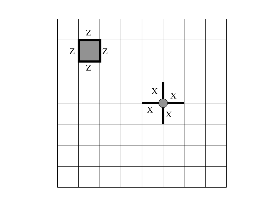
Figure 2.1: A plaquette operator $B$, comprising four $Z$’s, and a star operator $A$, comprising four $X$’s.

The toric code TOR$(k)$ uses $2k^{2}$ physical bits arranged in a $k\times k$ lattice (with edges identified) to encode two logical bits. Its stabilizer—i.e. the group of all transformations that do not affect the encoded information—is generated by star and plaquette operators

$$A_{s}=\prod_{+s}X\;\;\;\;\;\;\;\;\mbox{and}\;\;\;\;\;\;\;\;B_{p}=\prod_{\Box p}Z$$

respectively, where “$+s$” denotes the four edges emanating from vertex $s$ and “$\Box p$” denotes the four edges enclosing face $p$ (see Fig. 2.1). The code subspace is that fixed by $A_{s}$ and $B_{p}$ for all $s$ and $p$. Note that any $A_{s}$ shares either zero or two edges with any $B_{p}$, so all the stabilizer operators commute. Because of the two operator identities $\prod_{s}A_{s}=1$ and $\prod_{p}B_{p}=1$, only $2k^{2}-2$ of the stabilizer generators are independent, giving $2k^{2}-(2k^{2}-2)=2$ encoded qubits, i.e., a 4-dimensional code subspace. The connection to topology arises from the fact that the plaquette operators generate exactly the set of contractible loops of $Z$’s on the lattice (see Fig. 2.2). Likewise, the star operators generate exactly the the set of contractible loops of $X$’s on the dual lattice (the lattice obtained by rotating every edge by $90^{\circ}$ about its midpoint).

To see how this is reflected in the assignment of logical basis elements (“codewords”), let us find them explicitly. Consider the (unnormalized) state

$$|\bar{0}\bar{0}\rangle\equiv\prod_{s}\left(1+A_{s}\right)|0\cdots 0\rangle=\left(1+\sum_{s}A_{s}+\sum_{s<s^{\prime}}A_{s}A_{s^{\prime}}+\cdots\right)|0\cdots 0\rangle$$

where $|0\cdots 0\rangle$ refers to all the $2k^{2}$ physical bits and the barred bit-values indicate logical qubits. Any $B_{p}$ applied to this state commutes through all $1+A_{s}$ factors and leaves $|0\cdots 0\rangle$ fixed, so $|\bar{0}\bar{0}\rangle$ is a +1 eigenstate of all the plaquette operators. $|\bar{0}\bar{0}\rangle$ is also fixed by each star operator because, $A_{r}$ commutes through all the $1+A_{s}$ factors until it finds $1+A_{r}$, and $A_{r}(1+A_{r})=1+A_{r}$. Thus $|\bar{0}\bar{0}\rangle$ can be taken as a codeword. To see the topological nature of this state expand the product as above. Each term in the sum represents a pattern of contractible co-loops (loops on the dual lattice) and the sum is equally weighted over all such patterns. In this sense, all “geometries” are summed over, leaving only topological information as far as error chains are concerned. Operating on $|\bar{0}\bar{0}\rangle$ with any contractible co-loop of $X$’s just permutes terms of the sum, leaving the state unchanged.

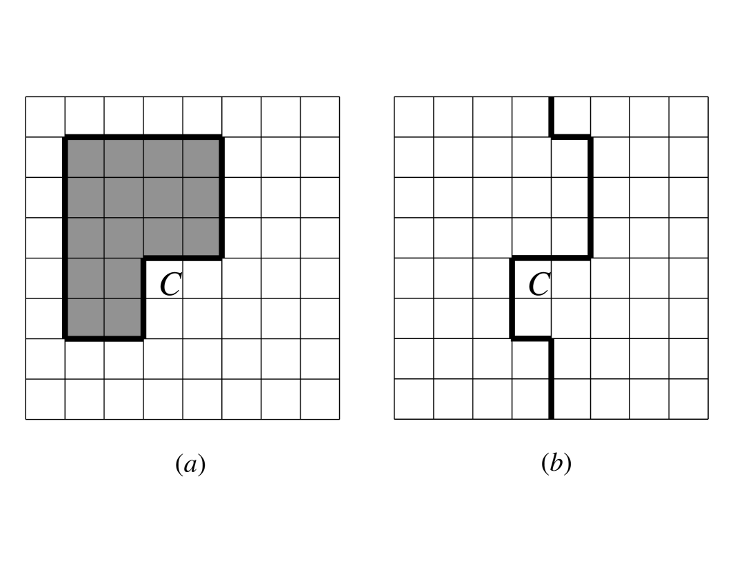
Figure 2.2: A contractible loop (a), and a non-contractible loop (b) on the lattice.

More generally, any loop of $Z$’s or co-loop of $X$’s, contractible or not, commutes with all the stabilizer operators. If the loop or co-loop is contractible it fixes all codewords, but if non-contractible it non-trivially transforms the code subspace. In fact we can take $X_{1}|\bar{0}\bar{0}\rangle$, $X_{2}|\bar{0}\bar{0}\rangle$, and $X_{1}X_{2}|\bar{0}\bar{0}\rangle$ as the three remaining codewords, where $X_{i}\equiv\prod_{c_{xi}}X$ is given by a non-contractible co-loop of $X$’s running across the lattice horizontally along the path $c_{x1}$ or vertically along $c_{x2}$ (see Fig. 2.3). (Here the index $i$ refers to lofical not physical qubits.) Thus $X_{1}$ and $X_{2}$ act as the logical $X$’s for bits 1 and 2. The logical $Z$’s are given by $Z_{i}\equiv\prod_{c_{zi}}Z$, a non-contractible loop of $Z$’s running horizontally ($i=2$) or vertically ($i=1$) across the lattice. Note that $c_{xi}$ and $c_{zi}$ run in perpendicular directions so that $X_{i}$ and $Z_{i}$ anticommute. Also note that these constructions only depend on topology: the paths defining any of these operators may be “continuously” deformed without affecting their action on the code subspace since any such deformation corresponds to applying a contractible loop operator, which fixes all codewords.

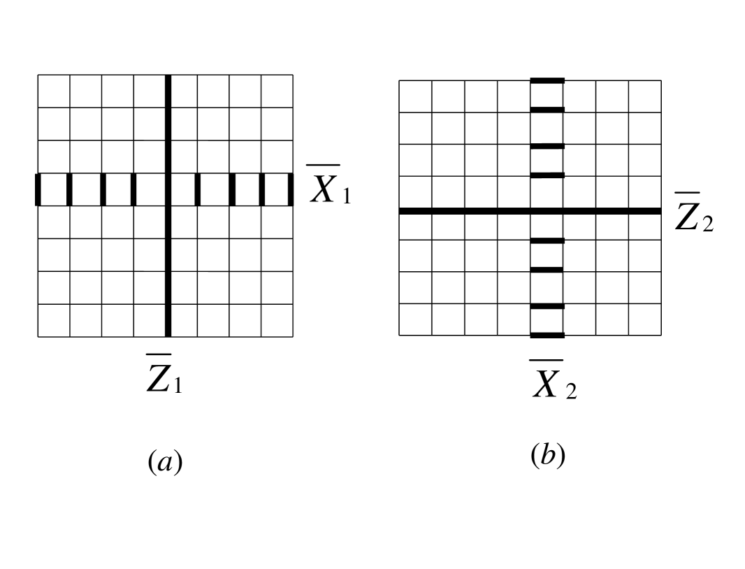
Figure 2.3: The logical $X$ and $Z$ operators for qubits 1 and 2. Each logical $Z$ is given by a non-contractible loop of physical $Z$’s, and each logical $X$ by a non-contractible co-loop of physical $X$’s.

Suppose we have a state in the code subspace and apply an open co-chain of $X$’s along some co-path $P$ between faces $q$ and $p$. This changes the quantum numbers for $B_{q}$ and $B_{p}$ from $+1$ to $-1$, generating “particles” at $q$ and $p$. Now the sum-over-geometries is such that the resulting state would be exactly the same if we had used not $P$ but some $P^{\prime}$ which is obtained by “continuously” deforming $P$ with its endpoints fixed. Information about which of the topologically equivalent co-paths is taken washes away in the superposition because $P$ and $P^{\prime}$ differ only by a contractible co-loop of $X$’s, which belongs to the stabilizer. Likewise, applying a chain of $Z$’s between vertices $r$ and $s$ generates a dual kind of particle at $r$ and one at $s$, with the same topological character. Given a lattice state we can measure all the star and plaquette operators to obtain a syndrome which just lists the locations of all the particles present on the lattice. To correct the errors indicated by the presence of the star (plaquette) particles we must group all the particles in pairs, connect each pair with a chain (co-chain) of our own, and apply $Z$ ($X$) operators to the qubits along these chains (co-chains). Leaving aside the possibility of measurement errors, which will be addressed below, this transforms an arbitrary pattern of errors into a number of closed loops on the (dual) lattice (see Fig. 2.4). What we want is that all these closed loops be contractible so that the logical qubits are left undisturbed. If one of the loops is non-contractible we will have unwittingly applied one of the $X_{i}$ or $Z_{i}$ operators to our state, causing an error in the encoded information.

In principle, it only takes $k/2$ errors lying along one non-contractible (NC) loop to undermine TOR$(k)$ irrespective of our particle pairing algorithm. But it would be exponentially improbable as $k$ gets large, that if just $k/2$ errors occur they would be positioned in just the right way to do this. In general, measuring all the star and plaquette operators will collapse the lattice state into a superposition of codewords all acted on by a definite set of single qubit phase ($Z$) and bit flip ($X$) errors. If decoherence/error processes act independently on separate qubits, and in a relatively uniform way, they will give rise to a certain probability, $p_{z}$, for each qubit to undergo a phase error, and perhaps a different probability, $p_{x}$, to undergo a bit error. Depending on $p_{x}$ and $p_{z}$ and on what algorithm we use to pair particles, there will be some probability that we are tricked into generating an NC loop when we think we have merely corrected errors. If this happens our state is corrupted, but we will see that such a recovery failure can be made exponentially improbable as $k$ increases, a result reminiscent of concatenated codes.

2.2 Repetition Code as a 1d Lattice Code

For practice and later reference let us examine the 1d equivalent of TOR$(k)$, which uses a circle of $k$ qubits instead of a $k\times k$ toric lattice. The plaquette operators do not exist here, and the star operator associated with vertex $s$ becomes the product of $X$’s over the two qubits touching $s$. In its own right this code, which is dual to repitition code discussed in Chapter 1, is worthless because a single bit flip error causes a logical bit flip error. But understanding the statistics of $z$-error chains will prove useful for analysis of TOR$(k)$.

Suppose our lattice code state is picked from an ensemble in which each physical qubit suffers a $z$-error with probability $p$, independent of all the other qubits. For example, we might have $\mathbf{n}=(0,1,1,0,0,0,1,0)$, which describes the 1d lattice (with ends identified)

— $$\leftrightarrow \leftrightarrow \leftrightarrow$$  — — —  —

where $\leftrightarrow$ indicates a $z$-error. Measuring the syndrome, we determine the locations of all $z$-error chain endpoints, in this case

—$$\cdot \cdot \cdot \cdot$$— —— — ———

We must now guess which endpoints are connected to which others and apply our own recovery chain of $Z$’s between each pair of “connected” endpoints to cancel the errors. In 1d there are only two possible guesses corresponding to two complementary patterns of errors on the circle. So if we guess wrong the combination of errors and recovery chains will encircle the lattice, giving $\mathbf{n}=(1,\ldots,1)$ hence a logical phase error. Otherwise we will have successfully corrected all the errors, giving $\mathbf{n}=(0,\ldots,0)$. Assuming the error probability $p$ is relatively small, the obvious algorithm for particle pairing would be to favor the minimum total length of recovery chains. (For a 2d analog of this minimum distance algorithm, see [22].) This algorithm, however, is highly non-local on the lattice; consider instead the following quasi-local alternative. First pair all particles separated by only one edge; contested pairings may be resolved randomly. Then pair any remaining particles separated by two edges, etc., until all particles are accounted for. In 1d this algorithm may produce a number of recovery chains which overlap hence cancel each other, always resulting in one of the two basic guesses.

The failure probability $F$, here referring to the probability of causing a logical phase error, derives from the set of all possible error configurations which can trick the algorithm into forming an NC loop of $z$-errors. In particular we have the bound

$$F\;=\;\langle n_{i}\rangle\;\leq\;k\sum_{n=n^{(k)}}^{\infty}h_{1}(n)p^{n}$$ (2.1)

where $h_{1}(n)$ is the number of different error chains that the algorithm can generate with a fixed number $n$ of $z$-errors and starting from a fixed vertex. In other words, $h_{1}(n)$ is the number of ways $n$ $z$-errors can trick the algorithm into flipping all the bits inbetween instead of correcting the erroneous bits themselves. The lower limit $n^{(k)}$ in the sum is the fewest number of errors necessary to cause the algorithm to generate an NC loop on a circle of size $k$. The ensemble average $\langle n_{i}\rangle$ refers to an arbitrary component of $\mathbf{n}$, evaluated after recovery chains have been applied. One might then expect $F$ is a kind of order parameter describing the topological order of error chains on the lattice. We shall see that for $p$ below a certain critical error rate $p_{c}$, our recovery algorithm maintains the lattice in a highly stable phase where $\langle n_{i}\rangle\ll 1$ so NC loops are very unlikely. In the thermodynamic limit $k\rightarrow\infty$, $\langle n_{i}\rangle=0$ in this phase, but what we want to know is exactly how small $\langle n_{i}\rangle$ is as a function of $k$.

To study $F$ let us first calculate $n^{(k)}$, or equivalently calculate the maximum length $l(n)$ of an $[n]$-chain—that is, an error chain generated by our algorithm and containing $n$ errors. Clearly $l(2)=3$, since two lone errors can be separated by at most one edge if they are to be paired by our algorithm. This makes the $[2]$-chain $\leftrightarrow$ — $\leftrightarrow$ where the middle link is a recovery chain. Now if we take two of these $[2]$-chains and join them through the longest possible recovery chain (itself 3 edges long), what we have is the longest possible $[4]$-chain. We can continue to build up maximal $[2^{L}]$-chains in this highly symmetrical, Cantor set pattern, and we find $l(2^{L})=3^{L}$. Generating an NC loop requires an error chain of length at least $k/2$, so if $k/2$ is a power of 3 we have $n^{(k)}=(k/2)^{\beta}$ where $\beta=\log_{3}2\approx 0.6309$. If $k/2$ is not a power of 3, the maximum chain will have to involve asymmetric joining processes, which serve only to decrease its length relative to the Cantor chain trend. Thus $l(n)=n^{1/\beta}$ serves as an upper bound on chain length in general, but it will prove useful to have an explicit expression when $n$ is inbetween powers of 2.

Consider the sub-chain structure of the maximal $[2^{L}-2^{M}]$-chain. We may emulate the Cantor pattern by dividing the $2^{L}-2^{M}$ errors into two identical $[2^{L-1}-2^{M-1}]$-chains and extending the longest possible recovery chain between them. Iterate the process for each of these two chains, etc., until we have reduced the lot into $[2^{L-M}-1]$-chains and can go no further. Now it is not hard to determine $l(2^{N}-1)$. As the $2^{N}-1$ errors join in successive levels, they look just like a Cantor chain, except at each level there is always one runt sub-chain shorter than the rest. At the first level, $[1]$-chains join in pairs to become $[2]$-chains ($\leftrightarrow$ — $\leftrightarrow$), except one is left unpaired resulting in the runt $[1]$-chain at the second level. Now the $[2]$-chains join in pairs, except one joins the runt giving the runt $[3]$-chain ($\leftrightarrow$ — $\leftrightarrow$ — $\leftrightarrow$), etc. The number of edges lost at each level relative to the corresponding Cantor chain are as follows: 2 edges at the first level; another 2 edges at the second; and at an arbitrary level, a number of edges equal to the sum of all previous losses. Summing the series yields a total relative loss of exactly $2^{N}$ edges, so $l(2^{N}-1)=l(2^{N})-2^{N}=3^{N}-2^{N}$. Taking all of our $[2^{L-M}-1]$-chains as units in one big Cantor pattern, one finds

$$l(n)=(3^{L-M}-2^{L-M})3^{M}=3^{L}-\left({\textstyle\frac{3}{2}}\right)^{M}2^{L},$$ (2.2)

which is the desired expression for maximal chain length when $n=2^{L}-2^{M}$ is inbetween powers of 2, giving the correct results for the limits $M=1,L-1$. Note $l(n)\leq n^{1/\beta}$ with equality when $n$ is a power of 2.

To bound the chain counting function $h_{1}(n=2^{L})$, consider all ways an $[n]$-chain can be decomposed into an $[m]$-chain $S$ and an $[n-m]$-chain $S^{\prime}$ joined by a recovery chain $R$. Neither $S$ nor $S^{\prime}$ can contain any recovery chains longer than $R$, which means that $S$ cannot contain any recovery chains longer than $S^{\prime}$ itself and vice versa. Thus we can write

$$h_{1}(n)\leq\sum_{m=1}^{n-1}h_{1}(m|m_{<})h_{1}(n-m|m_{<})\cdot(m_{<}^{1/\beta}+1)$$ (2.3)

where $m_{<}$ is the lesser of $m$ and $n-m$, and “$|m)$” reads “given that there are no recovery chains longer than $m^{1/\beta}$,” which is the maximum length of an $[m]$-chain. The factor $m_{<}^{1/\beta}+1$ counts all possible recovery chains $R$, including the “0-chain.” To bound the sum, let us find the maximum value of $h_{1}(m|m_{<})h_{1}(n-m|m_{<})$ over all possible $m$ or, without loss of generality, over $1\leq m\leq n/2$. In general we expect the number of different chains to increase with increasing chain length, so we should find the $m$ which allows for the maximum possible summed length $l_{SS^{\prime}}$ of $S$ and $S^{\prime}$, corresponding to the two $h$ factors. For a given $m$ we have

$$l_{SS^{\prime}}(m)=l(m)+l(n-m|m).$$

We know $l(m)$ from (2.2), and we can calculate $l(n-m|m)$ by finding the error configuration which saturates the “$|m)$” constraint. This is done by dividing the $n-m$ errors into groups of $m$ errors, arranging errors within each group in the Cantor form, and linking these groups together through recovery chains of maximum length. Together with (2.2), and using $l(m)=m^{1/\beta}$, this yields

$$l_{SS^{\prime}}(m)=2\frac{n-m}{m}l(m)=\frac{2}{m}\left[(n-m)n^{1/\beta}-n(n-m)^{1/\beta}\right].$$ (2.4)

It is straight-forward to show this function is strictly increasing over $1\leq m\leq n/2$, so that the maximum is achieved at $m=n/2$, which choice should then also maximize $h_{1}(m|m_{<})h_{1}(n-m|m_{<})$. Using (2.3) and the fact that $h_{1}(m|m)=h_{1}(m)$ we have

$$h_{1}(n)\leq\Sigma_{1}(n)h_{1}(n/2)^{2}\;\;\;\;\;\mbox{where}\;\;\;\;\;\Sigma_{1}(n)\equiv\sum_{m=1}^{n-1}(m_{<}^{1/\beta}+1).$$

Iterating the bound yields

$$h_{1}(n)\leq\left[h_{1}(1)\prod_{L=1}^{\infty}\Sigma_{1}(2^{L})^{2^{-L}}\right]^{n}=(8.872\ldots)^{n}.$$ (2.5)

with the aid of some numerical evaluation. We might have put $h_{1}(1)=2$ but instead use $h_{1}(1)=1$ because 1d error chains cannot double-back on themselves. (At a chain’s starting point $h_{1}(1)=2$ holds, but this has exponentially small effect for a long chain.) Now (2.1) implies a concise bound on the (phase error) failure probability for this 1d algorithm:

$$F\leq k\left(\frac{p}{p_{c}}\right)^{(k/2)^{\beta}}$$ (2.6)

where the actual accuracy threshold $p_{c}$ is no less than $1/8.872$.

2.3 Recovery with Perfect Measurements

We must now extend the algorithm to 2d (again assuming no measurement errors), so that something like (2.6) applies to both $z$-errors and $x$-errors. To simplify analysis we make no use of correlations between phase and bit flip errors, so $x$-error correction on the dual lattice is formally identical to $z$-error correction on the lattice, and only the latter is addressed below.

“Two particles separated by a distance $l$ on the lattice” means that the shortest path between them contains $l$ edges. The locus of vertices equidistant from a given vertex looks like a diamond. So, given a particle $s$ in the algorithm’s $t$-th step, we need to search for partners over all vertices on a diamond of radius $t$ centered on $s$. As the algorithm proceeds from $t=1$, error chains close into loops and join with one another until no open chains are left (see Fig. 2.4).

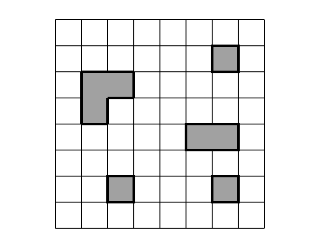
Figure 2.4: At the end of one recovery round, all open error chains have been transformed into closed loops on the lattice. Recovery is successfull if, as above, all these loops are contractible.

A bound on the failure probability is obtained as before, but we must calculate a new chain counting function $h_{2}(n)$ since a given 1d chain may wander across the 2d lattice along many different paths. Consider an $[m]$-chain with endpoints $r$ and $s$, which is to join an $[n-m]$-chain with endpoints $r^{\prime}$ and $s^{\prime}$. If the joining occurs through $s$ and $s^{\prime}$, then $s$ must be closer to $s^{\prime}$ than to $r$. So, taking $s$ fixed, $s^{\prime}$ must be somewhere within the diamond centered on $s$ and passing through $r$. This diamond has radius at most $m^{1/\beta}$ hence contains at most $2m^{1/\beta}(m^{1/\beta}+1)+1$ vertices. Thus in 2d we have

$$h_{2}(n)\leq\Sigma_{2}(n)h_{2}(n/2)^{2}\;\;\;\;\mbox{where}\;\;\;\;\Sigma_{2}(n)\equiv\sum_{m=1}^{n-1}2m_{<}^{1/\beta}(m_{<}^{1/\beta}+1)+1$$ (2.7)

and iteration gives

$$h_{2}(n)\leq\left[h_{2}(4)^{1/4}\prod_{L=3}^{\infty}\Sigma_{2}(2^{L})^{2^{-L}}\right]^{n}=(75.38\ldots)^{n}$$

with the aid of some numerical evaluation. Note we have halted iteration after reaching $h_{2}(4)$ in order to improve the bound. We have bounded $h_{2}(4)$ itself by using diagrams to count all possible $[4]$-chains. For example,

$$(\leftrightarrow\,\leftrightarrow)(\;\cdot\;+\;\mbox{---}\;+\;\mbox{---\,---}\;)(\leftrightarrow\,\leftrightarrow)=(4\cdot 3)(1+3+7\cdot{\textstyle\frac{4}{3}}\cdot{\textstyle\frac{1}{4}})(3\cdot 3)$$

is the contribution to $h_{2}(4)$ from the joining of two $[2]$-chains, each length 2. The numbers arise as follows: we start at some fixed vertex and have 4 choices for positioning the first error, leaving 3 choices for the second error. Our recovery chain may have length 0, 1, or 2, giving a number of choices equal to 1, 3, or 7 respectively. Then we have $3\cdot 3$ ways to position the next two errors. If the recovery chain is two edges long, however, there are $4\cdot 3$ ways to position these two errors, hence the factor of $\frac{4}{3}$ above. The factor $\frac{1}{4}$ arises from the fact that pairing ambiguities are resolved randomly by the recovery algorithm. If the recovery chain has length 2, there is only a 1/4 chance that the $[2]$-chains will join as above (for this to happen, one of the two interior vertices must be chosen first for pairing, and then it must be paired with the other interior vertex). We may compute three other diagrams allowing for either of the $[2]$-chains to have length 3, and we obtain the bound $h_{2}(4)\leq 4997$. (In counting arrangements of a length 3 chain we consider two separate cases, namely when the endpoints are separated by one edge and by three edges.)

The failure probability bound in 2d is thus

$$F\;\leq\;k^{2}\!\!\sum_{n=(\frac{k}{2})^{\beta}}^{\infty}h_{2}(n)p^{n}=k^{2}\left(\frac{p}{p_{c}}\right)^{(k/2)^{\beta}}$$ (2.8)

with critical probability $p_{c}\geq 1/75.38$. This result applies equally to $x$-error and $z$-error correction.

However, we shall see that this represents an over-estimate in regard to the exponent $(k/2)^{\beta}$. The bound (2.8) was derived by assuming that all chains of $(k/2)^{\beta}$ or more errors generate an NC loop, hence result in failure. But, for instance, of all the chains with $n=(k/2)^{\beta}$ errors only a few can generate an NC loop because every error must be placed in just the right spot along a perfectly straight line for the chain to achieve the necessary endpoint separation. In general, the fraction of chains starting from a given vertex and capable of generating an NC loop on our $k\times k$ lattice will be some function $f(n)$, tending to unity as $n$ gets large. This function should multiply the chain counting function $h_{2}(n)$ in our failure probability bound (2.8).

We know the $n^{(k)}=(k/2)^{\beta}$ contribution to $F$ should go like $p^{n^{(k)}}$ because once a starting point is picked, the positions of the $n^{(k)}$ errors are essentially all fixed if the chain is to generate an NC loop. Thus $f(n^{(k)})=(p_{c})^{n^{(k)}}$ to get the right term for $n=n^{(k)}$ in (2.8). Also $f(n)\leq 1$ by definition, so we can bound

$$f(n)\leq\left[p_{c}+\frac{n^{1/\beta}-k/2}{n_{0}^{1/\beta}-k/2}(1-p_{c})\right]^{n}$$

for some $n_{0}>(k/2)^{\beta}$. Using this in (2.8) with $h_{2}(n)$ multiplied by $f(n)$ and finding the maximum term in the sum allows us to sharpen (2.8) insofar as $n_{0}$ exceeds $(k/2)^{\beta}$. Physically $n_{0}$ represents the saturation point at which adding one more error to a chain stops having so great an effect on the chances of its being able to generate an NC loop. To get a hold on the value of $n_{0}$ first consider only geodesic error chains—chains of extremal length for fixed endpoints. Statistically this category will be dominated by nearly diagonal chains. But a diagonal chain must have length at least $k$ to generate a NC loop, so adding one more error will be irrelevant only if $n\geq k^{\beta}$. In general, error chains will be sub-geodesic, so that we expect the saturation point $n_{0}$ to exceed $k^{\beta}$. Using this as a bound, we find the maximum term in the sum of (2.8), if it exists, satisfies

$$\frac{p}{p_{c}}\leq\frac{k}{2l-k}\exp\left[-\frac{l}{\beta(l-k/2)}\right]$$

where $l\equiv n^{1/\beta}$ and we have neglected $O(p_{c})$ corrections. If this is satisfied by no $l<k$, the end term with $l=k$ is the maximum term. Since the above function is strictly increasing on $0\leq l\leq k$, this occurs if $p/p_{c}$ exceeds the right hand side above evaluated at $l=k$, which is $e^{-2/\beta}\approx 0.0420$. So we have the estimate

$$F\sim k^{2+\beta}\left(\frac{p}{p_{c}}\right)^{k^{\beta}}$$ (2.9)

where the exponent $k^{\beta}$ applies rather than $(k/2)^{\beta}$ if $p\geq 0.0420\,p_{c}$.

We have sought to test these results through numerical simulations of the recovery process. For a given torus size $k$, we perform $\sim 10,000$ individual recovery simulations for eight values of $p$ from 0.01 to 0.07. Each Monte Carlo run starts by generating a random pattern of errors, each edge with error probability $p$, and implements the expanding diamonds algorithm until all particles are paired. Recovery success or failure is determined by checking for NC loops. For each $p$, $F$ is just given as the failure frequency, which we fit with (2.9) as a function of $p$, for fixed $k$, yielding the $k^{\beta}$ exponent as a fitted paramter value in a log-log plot. (Here we neglect the prefactor $k^{2+\beta}$.) The logarithms of these extracted $k^{\beta}$ values are plotted against $k$ in Fig. 2.5. According to (2.9), the result should be a line with slope $\beta=\log_{3}2\approx 0.6309$. The measured slope is quite close: $0.627\pm 0.008$. The intercept—predicted as the log of the coefficient of $k^{\beta}$ in (2.9), hence zero—is measured to be $0.02\pm 0.03$. Measured values of the accuracy threshold $p_{c}$ for each $k$ are all comfortably consistent with the bound $p\geq 1/75.38$ obtained above.

Figure 2.5: Recovery failure rates $F$ as a function of lattice size $k$, obtained from Monte Carlo simulation of errors. The vertical axis is taken as the logarithm of $k^{\beta}$ values extracted from failure rate data and is effectively a double logarithm of $F$. The line represents our analytic result for the exponent $\beta=\log_{3}2$.

In picking the data to fit, we must select a maximum $p$ (or, equivalently, $F$) since the actual scaling for which (2.8) is a bound must break down at some $p$ greater than the bound obtained for $p_{c}$. Here, a cut-off at $F=.05$ was applied. We also select a minimum $F$ to limit Poisson scatter, chosen to minimize the standard error for our measured value of $\beta$. Scatter in the plot arises not only from Poisson fluctuations but also from the fact that actual values of $\beta$ for finite $k$ differ from the theoretical value $\log_{3}2$, which is really an asymptotic ($k\rightarrow\infty$) prediction. These finite $k$ effects involve the interpolation which must take place between Cantor chains whose lengths are all powers of 3.

2.4 Recovery with Imperfect Measurements

Until now we have assumed perfect syndrome measurements. But suppose we err in measuring each star operator $A_{s}$ with some probability $q$ (which might be the same order as the physical bit error probability $p$). This mistake would lead us to think a particle (“ghost particle”) exists at $s$ when there really is none, or that no particle exists at $s$ (“ghost hole”) when there really is one. Because the basic expanding diamonds algorithm becomes unstable when ghosts are introduced, we must modify it and apply our failure probability analysis (chain counting, etc.) to the modified version.

Imagine recovery (with measurement errors) via expanding diamonds. We would generate contractible loops, hence correct real errors, but recovery chains would also connect ghost particles to one another and to real particles. Once a chain connects to a ghost particle it can no longer propagate from that endpoint because there is no pre-existing error chain to continue it to another particle. So in addition to all the loops generated by recovery, the lattice would also be left with open chains that carry over to the next round as if they arose from spontaneous errors. Failure might occur, as before, by the generation of an entire NC loop in one recovery round or, now, over many rounds.

Unfortunately, the left-over chains quickly begin to dominate the failure rate. Suppose $q$ were small enough that in a particular round just two ghosts occurred. They would typically be separated by a distance O$(k)$ on the lattice. Since they are the only ghosts around, and open chains end only on ghosts, these two will be connected by a recovery chain, which will give an O$(1)$ chance of failure in the next round, independently of $k$. We cannot remedy this situation simply by repeating syndrome measurements a number of times to increase confidence in their results. The reason is that no matter how many times we repeat, there will always be processes involving just a few errors and ghosts (hence occurring with bounded probability) that corrupt the supposedly verified syndrome. For instance suppose, exactly half-way through a series of repeated rounds of syndrome measurement, a real error occurs with endpoints $r$ and $s$, but we err in measuring $A_{r}$. Majority voting after the final round would trick us into accepting $s$ as a real particle, but not $r$, effectively generating a ghost in our verified syndrome.

So we need a better algorithm. The first thing to realize is that we will inevitably leave open chains behind from one round to the next. The only way to prevent ghosts from generating long chains is to be suspicious of calls to connect widely separated particles. Suppose we are lead to consider generating a recovery chain between two particles separated by a distance $l$ in the $T$th round. Should we do it? If $l$ is large, the hypothetical chain is more likely a pair of ghost particles. But age is also important: the longer the particles have been around (left unconnected in previous rounds), the less likely they are to be ghosts. To keep track of particle age information, imagine a 3d lattice comprising 2d shelves representing successive rounds of syndrome measurement. Particles which are the endpoints of left-over chains will be registered from their birth to the present, forming vertical “world lines.” Pairing particles in the current round should be done by reference both to their spatial separation on the current 2d shelf and also their temporal separation, i.e., the number of rounds having elapsed between their respective births.

Ghosts can eclipse particles or join onto chains themselves, either way causing an age discrepancy between chain endpoints. However we attempt to correct these types of errors, there is always the additional possibility that we generate more of them ourselves. As we shall see, the kinds of processes which result in chains with large spatial displacements in 2d have analogs in 3d which generate large temporal displacements. And as before, the more defects (now including ghosts), the greater these separations can be. This suggests we treat temporal and spatial separations on the same footing: the algorithm should connect particles according to some definite combination of their spatial and temporal separations. A natural generalization of expanding diamonds is found by extending the 2d spatial metric on the lattice into a 3d space-time metric:

$$l_{\ast}=l+\alpha|\Delta T|$$ (2.10)

defines the 3d distance $l_{\ast}$ in terms of the spatial and temporal displacements $l$ and $\Delta T$. Diamonds in 2d become octahedra in the 3d lattice—an octahedron of radius $l_{\ast}$ being defined as the locus of points separated from a given vertex by a distance in $(l_{\ast}-1,l_{\ast}]$ according to the “$\ast$-metric.” Note these octahedra are squashed in the time direction by the factor $\alpha$. The value of $\alpha$ should be chosen according to the frequency of measurement errors relative to real errors. The smaller the rate of measurement errors, the less probable it is to generate age differences, so $\alpha$ should be higher.

At each step in a given round of recovery, scaled octahedra of fixed size are extended around the birth sites of particles currently available. Once a given particle’s octahedron encounters another particle’s birth site, the particles are paired and marked as “unavailable.” In 2d, a recovery chain would be applied between every particle pair. Now that is inadvisable due to the presence of ghosts. Having paired two particles $r$ and $s$, we should determine whether it is more probable that either (i) they are associated with two independent error chains whose other endpoints may have been obscured by ghosts, or (ii) $r$ and $s$ are in fact endpoints of the same chain. These probabilities are determined by the number of defects necessary to account for $r$ and $s$ under the assumption (i) or (ii), so we should find a 3d analog of the 2d result that at least $l^{\beta}$ errors are necessary to generate a chain of length $l$. As we shall see, the obvious generalization is approximately correct: $l_{\ast}^{\beta}$ effective defects, accounting through $\alpha$ for the different occurrence probabilities of real errors and ghosts, are necessary to generate a chain of length $l_{\ast}$ in the $\ast$-metric. In addition we will find, as would be expected, that at least $\sim T^{\beta}$ effective defects are necessary to maintain a chain in existence for $T$ rounds of recovery. These two results allow us to compare the two probabilities associated with cases (i) and (ii) above. This is done by comparing the number of effective defects required for each case, which are $T_{r}^{\beta}+T_{s}^{\beta}$ and $l_{\ast}^{\beta}$ respectively. Here $T_{r}$ and $T_{s}$ are the ages of the two particles $r$ and $s$, and $l_{\ast}$ is their $\ast$-metric separation. Once the 3d algorithm is done pairing particles, we apply a recovery chain between any given pair $r$ and $s$ whenever

$$l_{\ast}^{\beta}<T_{r}^{\beta}+T_{s}^{\beta},$$ (2.11)

which imposes a variable pairing-length cut-off on the algorithm.

Ambiguities in this 3d algorithm can arise in the process of identifying a current particle with a particular birth site. If errors occur on edges touching the original birth site, the particle’s vertical world line may continue on a vertex displaced from the original. Also, ghosts may eclipse a particle in a given set of rounds, leaving holes in its world line. These difficulties may be overcome on a round-to-round basis by simply requiring that the age ascribed to a vertex be conserved if its particle has been left over from previous rounds, i.e., has not yet been paired. If a left-over particle suddenly disappears, we probe with expanding diamonds around the eclipsed particle until we find an uneclipsed particle who could inherit the lost age. If the probe radius becomes large enough that the likelihood of eclipse due to ghost overtakes the likelihood of eclipse due to real errors, we conserve age by manually adjusting our syndrome record as if we had detected a particle at the vertex in question. (We continue to alter the syndrome by hand, if need be, until it becomes more likely that the hypothetical eclipsed particle is actually just a string of ghosts.)

Having now specified an algorithm in 3d, we must redo our failure rate analysis taking into account the time dimension and the leaving over of chains from one round to the next. Our method is basically the same as before, but the chain counting function $h_{2}(n)$ must be generalized to $h_{3}(n,\bar{n})$, where $n$ is still the number of real errors and $\bar{n}$ the number of ghost errors involved in the chain. The failure probability bound now becomes

$$F\leq k^{3}\sum_{n,\bar{n}}h_{3}(n,\bar{n})p^{n}q^{\bar{n}}$$ (2.12)

where the sum is taken over all pairs $(n,\bar{n})$ capable of generating an NC loop. Note that $h_{3}(n,\bar{n})$ counts chains involving errors which may have originated in previous rounds but have lasted through the present. We again obtain a recursion relation, now for $h_{3}(n,\bar{n})$ in terms of $h_{3}(m\leq n,\bar{m}\leq\bar{n})$, by considering all ways an $[n,\bar{n}]$-chain could be broken into an $[m,\bar{m}]$-chain $S$ and an $[n-m,\bar{n}-\bar{m}]$-chain $S^{\prime}$. Recall that in 1d the coefficient $(m_{<}^{1/\beta}+1)$ in the recursion relation (2.3) counted all the ways to choose the recovery chain connecting $S$ and $S^{\prime}$. In 2d this coefficient became the area of a diamond of radius $m_{<}^{1/\beta}$. And now in 3d it becomes the volume (in vertices) of a $\ast$-metric octahedron with radius $l_{\ast}(m,\bar{m})_{<}$, defined as the lesser of the two maximal $\ast$-metric lengths $l_{\ast}(m,\bar{m})$ and $l_{\ast}(n-m,\bar{n}-\bar{m})$. The new recursion relation is

$$h_{3}(n,\bar{n})\leq\sum_{m=0}^{n}\sum_{\bar{m}=0}^{\bar{n}}V(l_{\ast}(m,\bar{m})_{<})h_{3}(m,\bar{m})h_{3}(n-m,\bar{n}-\bar{m}).$$ (2.13)

Again we want to bound the sum by finding the maximum $h\cdot h$ term, now varying both $m$ and $\bar{m}$. By generalizing the 1d/2d relation $l(n)=n^{1/\beta}$ we will later see that chains can grow longest when ghosts are uniformly intermixed with real errors. It turns out they work best by cooperating, as opposed to, say, having all the real errors combine on one side of the chain and all the ghosts on the other. So a maximal chain, hence the maximum $h\cdot h$ term, must have uniform composition, $m/\bar{m}=n/\bar{n}$. Thus we can perform a calculation similar to that which gave (2.4), but with $l(m)\rightarrow l_{\ast}(m,(\bar{n}/n)m)$. In fact we need just observe, as will be shown later, that $l_{\ast}(m,(\bar{n}/n)m)$ grows faster with $m$ than does $l(m)$. Now $l_{SS^{\prime}}\rightarrow l_{\ast SS^{\prime}}$ is determined by the first equality in (2.4), which still holds in 3d, so that if $l_{SS^{\prime}}(m)$ was increasing on $1\leq m\leq n/2$ in 1d/2d, so must be $l_{\ast SS^{\prime}}$ in 3d. Thus the maximum is located at $m=n/2$, hence $\bar{m}=\bar{n}/2$, and (2.13) becomes

$$h_{3}(n,\bar{n})\leq\Sigma_{3}(n,\bar{n})h_{3}(n/2,\bar{n}/2)^{2},$$ (2.14)

where

$$\Sigma_{3}(n,\bar{n})\equiv\sum_{m=0}^{n}\sum_{\bar{m}=0}^{\bar{n}}V(l_{\ast}(m,\bar{m})_{<})$$

and the octahedral volume is given by

$$V(l_{\ast})=\sum_{\Delta T=-[l_{\ast}/\alpha]}^{[l_{\ast}/\alpha]}2\left[l_{\ast}-\alpha|\Delta T|\right]\left[l_{\ast}-\alpha|\Delta T|+1\right]+1,$$

with $[\cdots]$ denoting the greatest integer function. The chain counting function, hence the critical probabilities we shall soon bound, depend crucially on the function $l_{\ast}(n,\bar{n})$ which bounds the $\ast$-metric length of a chain containing $n$ real errors and $\bar{n}$ ghosts. As there is no compact expression in general, we need to investigate particular values of $n$ and $\bar{n}$.

The basic constraint on the length of an error chain is that none of its recovery chain components can be longer ($\ast$-metric) than either of the sub-chains which it joins. Consider the case $\bar{n}=0$. Even without any ghosts, the chain has extra freedom in the 3d lattice. Two purely spatial sub-chains may be joined by a purely spatial recovery chain (not exceeding either of their lengths), or they may trade space for time so that one chain occurs in a recovery round before the other. But no extra $\ast$-metric length can be gained by trading space for time, because for any “time-like” recovery chain there is always a “space-like” recovery chain of equal or greater length. This implies $l_{\ast}(n,0)=n^{1/\beta}$ just as in 2d. Now consider adding one ghost to a pre-existing error chain. If, for instance, a ghost at $s$ is connected to one of the chain’s endpoints, $s$ will show up as a new-born particle in the next round (which would not be the case had the ghost been a real particle, hence the endpoint of another chain). Thus, the ghost generates an age difference between the endpoints of that chain. Depending on the value of $\alpha$, the algorithm might permit a newborn ghost to join onto an older chain, causing a greater age difference. To simplify analysis let us fix $\alpha$ so that no newborn (i.e., age 1) particle may be joined with a particle of age greater than 2. Consider two particles of ages 1 and 3, separated by one edge. The condition that they cannot be joined by the algorithm is given by the pairing length cut-off (2.11) as $(1+2\alpha)^{\beta}>3^{\beta}+1^{\beta}=3$, comfortably satisfied by choosing $\alpha=2.4$. From this it follows by checking cases that the most an add-on ghost can extend a chain is to add a spatial separation of 2 edges and a final age difference of 2 rounds. If $n\gg\bar{n}$, the maximal chain has a “unit cell” comprising $n/\bar{n}$ real errors arranged in a Cantor chain with one ghost added on to the end. Unit cells are strung together as singe error units in the Cantor pattern, giving

$$l_{\ast}(n\gg\bar{n})=n^{1/\beta}+(2\alpha+2)\bar{n}^{1/\beta}$$

which retains the basic $1/\beta$ scaling exponent. Considering $n$ and $\bar{n}$ powers of two, one can check that this relation holds for $n\geq 4\bar{n}$. If $n$ and $\bar{n}$ in this range are not powers of two, the above may be taken as a bound. Also, one may experiment with smaller unit cells to obtain

$$l_{\ast}(n=2\bar{n})=(3+2\alpha)\bar{n}^{1/\beta}\;\;\;\;\;\;\mbox{and}\;\;\;\;\;\;l_{\ast}(n=\bar{n})=(2+\alpha)\bar{n}^{1/\beta}.$$

We may interpolate between the above three results by an appropriate step-function to achieve a bound on $l_{\ast}(n,\bar{n})$ for all $n\geq\bar{n}$. For $n=0$, one can investigate candidate maximal chains with a definite number of ghosts per unit cell. Each unit cell is gotten by saturating the cut-off (2.11). It turns out the true maximal chain has six per unit cell and scales according to

$$l_{\ast}(0,\bar{n})=(7+8\alpha)(\bar{n}/6)^{1/\beta}.$$

For $n\ll\bar{n}$, the maximal chain unit cell has $\bar{n}/n$ ghosts and one real error. It may be divided into many sub-units, each comprising six ghosts, except for one odd sub-unit which also has the one real error. Actually, we can make the unit cell a bit longer by giving one of the six ghosts in the odd sub-unit to a different sub-unit. This construction gives

$$l_{\ast}(n\ll\bar{n})=(6+2\alpha)n^{1/\beta}+(7+8\alpha)(\bar{n}/6)^{1/\beta},$$

which holds as a bound for $n<\bar{n}/6$. The $\ast$-metric lengths of chains for $\bar{n}/6\leq n<\bar{n}$ may be obtained by inspetion when $\bar{n}/n$ is integral. We will not overtax the reader with all these formulas. Again, $l_{\ast}$ is bounded by interpolating to a step-function for intermediate cases. Altogether we have a means of bounding $l_{\ast}(n,\bar{n})$ for any values of its arguments. Note that these expressions for $l_{\ast}(n,\bar{n})$ have been obtained by mixing the $n$ real errors and $\bar{n}$ ghosts uniformly, hence the “unit cells.” That uniform mixture maximizes $\ast$-metric length can be checked by comparison to the lengths, computed with the above formulas, of segregated chains comprising, e.g., one piece with only real errors and another with only ghosts.

Now that we have a handle on all the quantities involved in our recursion relation (2.14), let us use it to bound $h_{3}(n,\bar{n})$. First consider the case $\hat{n}\equiv n/\bar{n}\geq 1$. Recursion brings us down from $h_{3}(n,\bar{n})$ to the factor $h_{3}(n/\bar{n},1)$, assuming both $n$ and $\bar{n}$ are powers of two. And we have

$$h_{3}(\hat{n},1)\leq 2\,\Sigma_{3}(\hat{n},0)\,h_{3}(\hat{n}/2,0)\,h_{3}(\hat{n}/2,1),$$ (2.15)

expressing a division into two sub-chains of equal defect number, except that one has a ghost and the other does not. The factor of 2 arises because the one ghost may be put in either of the two sub-chains. We may recursively substitute for $h_{3}(\hat{n}/2,1)$ in this relation to obtain an expression involving no $h$ factors other than $h_{3}(2^{N},1)$ and those of the form $h_{3}(m,0)$. (The integer $N$ may be chosen freely.) The $h_{3}(m,0)$ terms may all be reduced to $h_{3}(2^{N},0)$ using the original relation (2.14) with $\bar{n}=0$. When account is taken of all the $\Sigma_{3}$ factors produced by these recursions, one finds the quantity $q^{\bar{n}}h_{3}(n\geq 2^{N}\bar{n})$ is bounded from above by

$$\left\{\left[\frac{\hat{n}q}{2^{N}}\frac{h_{3}(2^{N},1)}{h_{3}(2^{N},0)}\prod_{L=N+1}^{\infty}\Sigma_{3}(2^{L}\hat{n},2^{L})^{2^{-L}}\right]^{\frac{1}{\hat{n}}}h_{3}(2^{N},0)^{2^{-N}}\prod_{L=N+1}^{\log_{2}\hat{n}}\Sigma_{3}(2^{L},0)^{2^{-L}}\right\}^{n}$$ (2.16)

(For $\hat{n}\leq 2^{N}$ the second product over $L$ should be set to unity.) Note that the bracketed expression $\{\cdots\}$ has the form $g(\hat{n},q)$, depending on $n$ and $\bar{n}$ only through $\hat{n}\equiv n/\bar{n}$. Strictly, we have obtained (2.16) only for $\hat{n}$ a power of two. Calculating intermediate cases, we would expect to find a correction to (2.16) resembling the correction (2.2) to our 1d/2d scaling law $l(n)=n^{1/\beta}$. We can now express the $n\geq\bar{n}$ part of the sum in (2.12) as

$$\sum_{n\geq\bar{n}}(q^{\bar{n}}h_{3}(n,\bar{n}))p^{n}=\sum_{\hat{n}\geq 1}\sum_{n}(g(\hat{n},q)\,p)^{n}.$$

where the first sum is only over pairs $(n,\bar{n})$ capable of generating NC loops, which we have converted to a sum over $\hat{n},n$. For a given $\hat{n}$ the sum over $n$ begins at a definite value $n=(k/2\gamma(\hat{n}))^{\beta}$, which is determined by one of the $l_{\ast}(n\geq\bar{n})$ formulas as the minimum $n$ such that $n$ real errors together with $\bar{n}=n/\hat{n}$ ghosts can generate a chain of spatial length $k/2$. In particular, $\gamma(\hat{n})$ is maximum at $\hat{n}=1$ where the $l_{\ast}(n=\bar{n})$ formula gives $\gamma=2+\alpha$. Considering the sum over $n$ as already performed, terms in the remaining sum over $\hat{n}$ depend on $p$, $q$, and $\hat{n}$ alone. Fixing $p$ and $q$, the maximum term will occur at some $\hat{n}=\hat{n}(q,p)$, which then determines an asymptotic ($k\rightarrow\infty$) critical probability $p_{c}(q,p)=1/g(\hat{n}(q,p),q)$ and scaling exponent through $\gamma(\hat{n}(q,p))$.

The case $n\leq\bar{n}$ follows in the same way, and a bound is obtained for the quantity $p^{n}h_{3}(n\leq\bar{n})$ which is exactly the expression (2.16) with $q\leftrightarrow p$ so that the two arguments are interchanged in all the $h$ and $\Sigma$ functions, $n\leftrightarrow\bar{n}$, and $\hat{n}\rightarrow 1/\hat{n}$. We may denote the resulting expression inside $\{\cdots\}$ by $\bar{g}(\hat{n},p)$, which gives rise to a measurement error critical probability $q_{c}(q,p)=1/\bar{g}(\hat{n}(q,p),p)$ and scaling exponent $(k/2\bar{\gamma})^{\beta}$. Thus the failure rate bound in 3d is

$$F\;\;\leq\;\;k^{3}\left[\frac{p}{p_{c}(q,p)}\right]^{\left(\frac{k}{2\gamma}\right)^{\beta}}+k^{3}\left[\frac{q}{q_{c}(q,p)}\right]^{\left(\frac{k}{2\bar{\gamma}}\right)^{\beta}}$$ (2.17)

where $\gamma,\bar{\gamma}\leq 2+\alpha$ both depend on $(q,p)$. The accuracy threshold is no longer a single point $p_{c}$ as in the case of no measurement errors, but is now a definite curve in the $qp$-plane—the boundary of the region lying underneath the two curves given implicitly by $p=p_{c}(q,p)$ and $q=q_{c}(q,p)$. This is a sort of phase boundary between the well-ordered, sub-threshold state where long error chains are exponentially improbable and the disordered state where long chains occur frequently and the encoded information is quickly corrupted.

To obtain this threshold curve one could calculate $p_{c}(q,p)$ and $q_{c}(q,p)$ directly, or choose a far less intensive method which is to calculate $g(\hat{n}\geq 1,q=1)$ and $\bar{g}(\hat{n}<1,p=1)$ for a number of values of $\hat{n}$ and use the fact that $g(\hat{n},q)=g(\hat{n},1)q^{1/\hat{n}}$ and $\bar{g}(\hat{n},p)=\bar{g}(\hat{n},1)p^{\hat{n}}$ to obtain curves in the $p$-$q$ plane corresponding to thresholds for individual contributions to $F$ from chains with fixed error-ghost composition $\hat{n}$. The region underlying all these curves is exactly the sub-threshold region. We have numerically calculated $g(\hat{n}=2^{M},1)$ and $\bar{g}(\hat{n}=2^{-M},1)$ for $M=0,1,\ldots,16,\infty$. In these calculations we set the recursion limit $N$ in (2.16) by $N=\min\{M,4\}$. This means we need to calculate bounds on $h_{3}(2^{L},m)$ and $h_{3}(m,2^{L})$ for $L=0,1,2$; $m=0,1$. We reduce $h_{3}(4,1)$ by one application of (2.15), and $h_{3}(1,4)$ by one application of the analogous relation with $q\leftrightarrow p$. Bounds on the remaining $h_{3}$’s are again obtained by inspection of diagrams. For example, the diagramatic break-down of $h_{3}(4,0)$ is almost identical to that of $h_{2}(4)$ in 2d which we have already calculated. The only additions are diagrams involving errors distributed over multiple rounds of recovery. In particular, by reference to (2.10) and (2.11) one finds

$$h_{3}(4,0)=h_{2}(4)+(\leftrightarrow\,\mbox{---}\,\leftrightarrow)(\leftrightarrow\,\leftrightarrow)=4997+(4\cdot 3\cdot 3){\textstyle\frac{1}{4}}(4\cdot 3)=5105$$

where the chain within the first parentheses occurs one round before the chain within the second.

The values obtained for $\log(g)$ and $\log(\bar{g})$ are roughly linear in $1/\hat{n}$ and $\hat{n}$ respectively. The points $\hat{n}=2^{\pm M}$ chosen for these calculations possess high symmetry in the same way the points $n=2^{M}$ posses high symmetry in regard to the 1d/2d scaling function $l(n)$. Expecting for $g$ and $\bar{g}$ a similar kind of peak-structure around points of high symmetry as was observed in (2.2) for $l(n)$, we use linear interpolation for reasonable bounds on points intermediate between $\hat{n}=2^{\pm M}$ for $M=0,1,\ldots,16,\infty$. The resulting sub-threshold region is a foot-like area with its heel at the origin of the $qp$-plane (see Fig. 2.6). The phase boundary has three main parts, coming respectively from the contributions to $F$ corresponding to $\hat{n}=2,1,\mbox{ and 1/2}$, hence to chains of twice as many real errors as ghosts, of equally as many, and of half as many. The ankle is cut-off around $p=1/114.5$ by threshold curves for higher $\hat{n}$, hence more real errors, and the toes are cut-off around $q=1/115.3$ by curves for lower $\hat{n}$, hence more ghosts. These two values, then, represent the limiting accuracy thresholds achieved by the 3d “expanding octahedra” algorithm.

Figure 2.6: Accuracy threshold for recovery with faulty syndrome measurements represented as a phase boundary in the $qp$-plane. Each curve correesponds to error chains of a different composition $\hat{n}$, and the region underneath them all is that in which recovery is stable.

Now these exponents $(k/2\gamma)^{\beta}$ and $(k/2\bar{\gamma})^{\beta}$ are over-estimates, just as in 2d, due to the conservative assumption that any chain with a sufficient number of defects to form an NC loop will in fact do so. Recall in 2d consideration of the saturation point $n_{0}$ for geodesic chains suggested a conservative estimate of $F$ with exponent $(k/2)^{\beta}$ replaced by $k^{\beta}$ if $p\geq 0.0420\,p_{c}$. The same arguments apply in 3d, except geodesics may now move in the time direction as well. For a long geodesic chain, the 2+1 components of its displacement will each average to the same $\ast$-metric length. An NC loop can be generated when this length is $k/2$, so the total $\ast$-metric length of the chain is $3k/2$. Consider a definite radial line in the $(q,p)$ plane, on which $F$ is dominated by one particular $\hat{n}$ threshold. The saturation point analysis here is essentially the same as in 2d, and one finds the 3d exponents are improved to $(3k/2\gamma)^{\beta}$ and $(3k/2\bar{\gamma})^{\beta}$ if $p/p_{c}\geq 2e^{-2/\beta}\approx 0.0840$.

Numerical simulations with measurement errors are performed, leaving over chains from one round to the next. Recovery failure is assumed to occur if either an NC loop occurs or an error chain’s endpoints achieve a spatial separation of $k$ or more (which would shortly lead to an NC loop). After a failure, the lattice is reset to an error-free state, and recovery resumes. The failure rate is calculated as the the number of failures divided by the total number of rounds. To speed up simulations the expanding octahedral radii $l_{\ast}$ are incremented in steps larger than one depending on the ages of current particles. The increment is chosen so that only five steps are necessary per round independent of $k$, which was not observed to significantly affect performance. In these simulations we set $q=p/2$, with $k$ ranging from 10 to 60 for each $(q,p)$. The critical behavior is understood from our $qp$-plane (Fig. 2.6) by walking out from the origin along the line $p=2q$. This line happens to cross the phase boundary right near the edge of the segment dominated by the $\hat{n}=1$ threshold curve, corresponding to $\gamma=2+\alpha$. Since this is the maximum possible $\gamma$, $F$ will indeed be dominated by the $\hat{n}=1$ threshold in this edge region. Thus our theoretical prediction here, with saturation improved exponent, is

$$F\sim\left[q\,p\,h_{3}(1,1)\prod_{L=1}^{\infty}\Sigma_{3}(2^{L},2^{L})^{2^{-L}}\right]^{(3k/2\gamma)^{\beta}}\approx\left(\frac{p}{p_{c}}\right)^{1.0143\,k^{\beta}}$$

neglecting a polynomial prefactor. Here $p_{c}$, specific to the case $p=2q$, is at least $1/329.8$. This result for the exponent $(3k/2\gamma)^{\beta}$ is shown as a line alongside the simulation data in Fig. 2.7. The agreement here is not as good as in the absence of measurement errors, but that is to be expected given the added complications of the 3d algorithm. These would presumably tend to enhance the finite $k$ deviations from our asymptotic predictions. Still, our conservative estimate is good, with only a couple of the data points completely below the line (indicating failure rates above the estimate).

Figure 2.7: Recovery failure rates $F$ as a function of lattice size $k$ from Monte Carlo simulations including measurement errors (“ghosts”) alongside the theoretical prediction (line).

Bravyi and Kitaev [20] and, independently, Freedman and Meyer [10] have exhibited lattice codes like TOR$(k)$ but using simply connected lattices with boundary in the plane. This presents a major advantage for any ultimate experimental implementation. A recovery algorithm appropriate to these codes is just that given above, but modified to account for the possibility of error chain endpoints being hidden on the boundary. Since the boundary is asymptotically irrelevant to scaling properties of lattice codes, the above results would seem to carry through.

2.5 Lattice Codes on High Genus Surfaces

In Kitaev’s topological framework for quantum codes, the basic determiner of a code’s fidelity $1-\epsilon$ in maintaining encoded information is the length $L$ of (i.e., the number of edges contained in) the shortest possible non-contractible loop on the lattice. In particular, we have seen that the code’s failure probability scales as

$$\epsilon\sim(p/p_{c})^{KL^{\beta}}$$ (2.18)

where $p$ is an error probability for physical qubits, and $p_{c}$, $\beta$, and $K$ are parameters depending on the particular error correction algorithm used.

$2N$ qubits may be encoded in $N$ separate lattices, each with fidelity given above. What we will show here is that, if instead of $N$ separate lattices we combine them into one large lattice on a high genus surface constructed by a certain method, the information rate and/or fidelity may be improved as the number of encoded qubits increases.

As a motivating example, consider joining two $L^{\prime}\times L^{\prime}$ toric lattices by removing a $L^{\prime}/2\times L^{\prime}/2$ square from each and sewing together the perimeters of the resulting square holes; it is straightforward to define a code on this new lattice preserving the total number, four, of encoded qubits. Taking $L^{\prime 2}\approx 4L^{2}/3$, the number of physical qubits is nearly the same as for two separate $L\times L$ lattices, but the minimum length of non-contractible loops is now $\approx 2L/\sqrt{3}$, improving the code’s fidelity.

This suggests, given $N$ separate $L\times L$ toric lattices, we combine the $2L^{2}N$ physical qubits into one large high-genus surface on which each torus becomes one handle. We can increase the code’s fidelity by the following construction. Cut each handle through its width, along a “w-loop” (see Fig. 2.8), giving two loose ends per handle. Then randomly re-pair the set of $2N$ loose ends and rejoin each pair.

Figure 2.8: A simple w-loop and simple l-loop are shown on two different handles.

Before cutting and rejoining w-loops, the lengths of length-wise “l-loops” had been as small as $L$; now the shortest simple l-loops for a typical handle will have length $\sim LN$. If each handle is made to encode a qubit with $Z$ operator given by an l-loop, it appears the chances of a $Z$ error to these encoded qubits has been markedly diminished. One might like to say this error probability is now exponentially small in $(LN)^{\beta}$. But there are more complicated l-type loops with lengths much smaller than $LN$; each such loop involves many handles. The minimal l-loops of this kind determine the encoded $Z$ error probability of a lattice code based on this large surface. Let us first determine the lengths of minimal l-loops, then symmetrize the construction of our surface to handle encoded $X$ errors as well.

To characterize the minimal l-loops we will calculate some geometrical properties of our high-genus surface, on which it will be convenient to recall the square lattice of qubits. If each handle connects to the surface through a square patch, the lattice will be locally identical to a simple square lattice except at the corners of a square patch. Each corner vertex has valence (number of edges containing it) equal to five not four, giving five quadrants of 2d space (see Fig. 2.9). The corner constitutes a kink of negative curvature on the otherwise flat lattice.

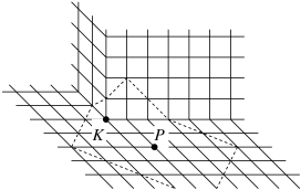
Figure 2.9: The kink $K$ appears at the base of a handle. A diamond (dashed line) centered at $P$ and containing $K$ is shown.

Around some vertex $P$ draw a small diamond. As its radius $r$ increases, the diamond will encounter handles over which it must climb, extending out to new places on the surface. From an intrinsic perspective, the diamond merely sees an occasional kink, from which emanates an extra quadrant of space. Having passed over a kink and encroached into its extra quadrant, the diamond’s perimeter will become larger than it would be apart from the kink. It is not hard to see the perimeter will contain an additional $r-r_{\mathrm{k}}$ vertices, where $r_{\mathrm{k}}$ is the distance from $P$ to the kink.

As the diamond expands, it encounters more kinks and its perimeter grows even faster. Moreover, all kinks contribute independently to the perimeter. Assuming a constant density, $8/L^{2}$ per vertex, of kinks on the lattice, the perimeter $c(r)$ approximately satisfies the recursion relation

$$c(r)=4r+\frac{8}{L^{2}}\sum_{r_{\mathrm{k}}=0}^{r}c(r_{\mathrm{k}})\cdot(r-r_{\mathrm{k}}),$$ (2.19)

obtained by adding independent contributions from all kinks within the diamond; $c(r)=4r$ would be the result in flat space. The above relation can be cast as a second order finite difference equation, with initial conditions, whose solution is approximately

$$c(r)=L\sqrt{2}\sinh\left(\sqrt{8}\,r/L\right).$$ (2.20)

To obtain the minimal l-loop length for a given handle $H$, consider the set of open paths of length $r$ and starting at some vertex $P$ around the base of $H$. As $r$ increases, the diamond forming the outer boundary of this set will be pushed across various handles to random new places on the surface, gradually filling it up. Once a path encounters the other end of $H$, it can be closed across $H$ to form an l-loop. The chances there will be such a path become significant only when the area of our $r$-diamond approaches a significant fraction of the total surface area, $L^{2}N$. Obtaining the diamond’s area by summing (2.20), this condition is found to be $r\sim L\log N/\sqrt{8}$, which thus gives the minimal l-loop length for almost all handles on the surface. As for the other handles, one can either attempt to re-pair them or simply discard them (close and eliminate them as handles).

The probability of encoded $Z$ errors associated with l-loops is thus exponentially small in $(L\log N)^{\beta}$; however no improvement has been achieved for $X$ error correction. To symmetrize the above construction, we simply add an additional cut-and-pair step. Previously we had cut along a w-loop on each handle and then re-paired all the cuts. Now we cut along an l-loop, which may be as short as $\sim L\log N$, and randomly re-pair as before. There is no longer a simple w-loop that can be drawn encircling a given handle. A w-loop must proceed across many of these cuts before it can close on itself non-contractibly. Topologically, this new step is identical to the previous one but with the surface turned inside-out. The effect of these new cuts and joins is just a doubling of the kink density to $16/L^{2}$ in (2.19), giving the minimal loop length—now for l-loops and w-loops—as $\sim L\log N/4$.

This result can be applied either as an improvement to the $L,N$-dependence of the lattice code’s fidelity at fixed information rate, an improvement to the information rate at fixed fidelity, or as a simultaneous improvement to both. But there is another parameter to be considered: the accuracy threshold $p_{c}$. Indeed, this convoluted surface topology suggests a greater variety of possible catastrophic error processes (long error chains) which would tend to worsen the threshold.

Nevertheless, as $L$ is increased at fixed $N$ the error processes affected by the convoluted topology will only be those involving longer and longer, hence less and less probable, error chains. As $L$ gets large the threshold will then tend back to its original value. For the quasi-local error correction algorithm presented above with $\beta=\log_{3}2$, the effect of convoluted topology is to multiply our bound on the threshold $p_{c}$ by

$$\sim\prod_{k=1}^{\log_{3}(L\log N)}\left[\frac{2(3^{k})^{2}}{a(3^{k})}\right]^{(1/3^{k})^{\beta}}\approx 8e^{-12(\log N)^{1-\beta}/L^{\beta}}$$

where $a(r)$ is the circular area obtained by summing (2.20). This means that $N$ should not be increased faster than $\log N\sim L^{\beta/(1-\beta)}$ or else the code’s accuracy threshold may be greatly diminished. Thus the fidelity $1-\epsilon$ from (2.18) will scale as

$$-\log\epsilon\sim(L\log N)^{\beta}\sim L^{\beta/(1-\beta)}\,.$$

Were we to naively put $\beta=1$ above, we would find that there is no restriction on how $N$ scales with $L$—unbounded gains could be had by increasing $N$ at fixed $L$ without serious damage to the accuracy threshold. In fact a different, global recovery algorithm does have $\beta=1$, and explicit consideration of its performance under convoluted topology corroborates this result. Bounds on the threshold are obtained here by counting certain classes of paths on the lattice [15]. For instance, the number of length $r$ paths with given starting point on a flat square lattice is $4^{r}$. On our curved lattice, some vertices (the kinks) have valence 5, so the number of walks is bounded by $v^{r}$ with $4<v<5$. The effect of convoluted topology on a threshold bound based on this counting would be to multiply it by the near-unity factor $4/v$.

We have thus shown how to achieve gains in the fidelity and/or efficiency of storing quantum information by encoding many qubits in one block of a topological quantum code. The code involves a lattice of qubits on a 2d surface of highly convoluted topology. As more encoded qubits are added, keeping fixed the number of physical qubits per encoded qubit, asymptotically significant gains are obtained in the code’s fidelity. This is an economy of scale in the error correction hardware independent of any software gains achieved by compressing redundancy within the encoded information itself, as in Shannon’s coding theorems and their quantum equivalents [16], which rely on the encoded qubits’ occupation of “typical” subspaces in the many-qubit Hilbert space.

One beneficial feature of the original topological codes is that error correction operations are local on the lattice; however, this is also a limitation. The convoluted topology of the above construction, which effectively destroys the codes’ locality, is a way of overcoming this limitation (and sacrificing the associated benefit).

Chapter 3 Unconcatenated Quantum Computing

3.1 Encoded Computation: The Toffoli Gate

So far we have mainly addressed error correcting codes in terms of storing quantum information. To realize an actual quantum computer, it is necessary to show how quantum gates may be performed on encoded qubits. While specific methods have been invented for a large class of concatenated quantum codes, the lattice codes we have discussed were designed specifically to obviate something inherent in the concatenation process: the generic reliance on highly non-local gates. We must therefore attempt to devise methods for performing encoded gates that do not rely on the recursive structure of concatenated codes.

Most known quantum error correcting codes (concatenated and lattice codes alike) can be defined by a set of operators, the stabilizer, each of which fixes every codeword. For a number of stabilizer codes capable of simple operations, like a bit flip $X_{a}$ or phase flip $Z_{a}$ on logical qubits $a,b,\ldots$, it is also known how to perform any “normalizer” operation—i.e. one that can be composed from the C-NOT, which we will now denote by $\dot{X}_{ab}$, the $\pi/2$ phase shift, and the Hadamard rotation $R_{a}$. Normalizer operations alone, however, are insufficient for universal quantum computation; a quantum computer with only normalizer operations can be simulated in polynomial time by a classical machine [17]. A genuine quantum computer is realized either by the addition of a non-trivial one or two-qubit gate, like a single qubit rotation by an irrational multiple of $\pi$, or of a three-qubit gate like the Toffoli (controlled-controlled-NOT), which flips the third qubit whenever the first two are each $|1\rangle$. Because the necessary one or two-qubit gates require rotations (e.g., $e^{\mathrm{i}\theta X}$) involving SU(2) angles that must be precisely tuned, they cannot be implemented fault-tolerantly. Small errors in these angles are inevitable and will gradually accrue until the computation veers completely off course. The Toffoli, on the other hand, like the C-NOT, does not involve any such rotations and therefore is suitable for fault-tolerant implementation.

Peter Shor has given a procedure [11] for performing a Toffoli given the ancilla state

$$|\psi_{3}\rangle\equiv|000\rangle+|001\rangle+|010\rangle+|100\rangle,$$ (3.1)

which means essentially that possessing the tripartite entanglement of this state is equally as powerful as being able to perform a Toffoli gate. Let us review Shor’s procedure (actually, a similar procedure that is equivalent to Shor’s).

As motivation, first consider the following construction, which uses one ancilla bit $c$. Letting $c$ start as $|0\rangle$, suppose we could perform a majority vote on $A\,B\,c$ so that, for example, $|010\rangle\rightarrow|000\rangle$ and $|110\rangle\rightarrow|111\rangle$. Equivalently, one might majority vote, but only carry out the effect on $c$, leaving $A$ and $B$ unchanged, so $|010\rangle\rightarrow|010\rangle$ and $|110\rangle\rightarrow|111\rangle$. Now just C-NOT $c$ into $C$ and disentangle $c$ from $A\,B\,C$. The result is exactly a Toffoli on $A\,B\,C$.

To majority vote on $A\,B\,c$, one measures $Z_{A}Z_{B}$ and $Z_{B}Z_{c}$. If both measurement results are $+1$, $A\,B\,c$ are already unanimous. Otherwise, the measurement results will reveal which bit is the odd-one-out. Unfortunately, these measurements have also revealed information about the initial state $A\,B$, in general collapsing it, inconsistent with the desired Toffoli gate, a linear operation. The solution is to perform a majority vote not directly on $A\,B\,c$ but on three ancilla qubits, which are first entangled with $A\,B$. Here is where $|\psi_{3}\rangle$ enters.

Given some arbitrary state of $A\,B\,C$, prepare $a\,b\,c$ in $|\psi_{3}\rangle$ and perform the following operations: (I) C-NOT $A$ into $a$ and $B$ into $b$, and (II) majority vote on $a\,b\,c$ (by measuring $Z_{a}Z_{b}$ and $Z_{b}Z_{c}$ and flipping the odd-bit-out if necessary). Suppose, for example, the measurement results from (II) are $Z_{a}Z_{b}=-1$ and $Z_{b}Z_{c}=+1$. All but 8 terms will be collapsed away of the total $2^{3}\times 4=32$ terms in the initial 6-qubit state. These 8 terms, as they undergo (I) and (II), are (suppressing bra-ket notation):

$$\begin{array}[]{rcccr}&\mbox{I}&&\mbox{II}\\ \vskip 3.0pt plus 1.0pt minus 1.0pt00C_{0}100&\rightarrow&00C_{0}100&\rightarrow&00C_{0}000\\ \vskip 3.0pt plus 1.0pt minus 1.0pt01C_{1}001&\rightarrow&01C_{1}011&\rightarrow&01C_{1}111\\ \vskip 3.0pt plus 1.0pt minus 1.0pt10C_{2}000&\rightarrow&10C_{2}100&\rightarrow&10C_{2}000\\ 11C_{3}010&\rightarrow&11C_{3}100&\rightarrow&11C_{3}000\end{array}$$

where $C_{i}=0,1$. Note that all of the 8 possible bit values for $A\,B\,C$ are equally represented, so that all information in the initial superposition of $A\,B\,C$ is preserved (albeit decoherently). Now C-NOT $c$ into $C$. From the above table, this will flip $C$ iff $A\,B$ are $01$—not iff $A\,B$ are $11$, as desired for the Toffoli. Applying $\dot{X}_{BC}$ then gives the desired result. Finally, $A\,B\,C$ must be disentangled from the ancillas $a\,b\,c$ to restore the coherence of the original state. This is accomplished by applying $\dot{X}_{ab}$ and $\dot{X}_{ac}$ and then measuring $X_{a}$. If the result is $+1$, $A\,B\,C$ are disentangled. If $-1$, a phase error on the $A\,B=01$ term has been introduced; it may be corrected by applying $X_{A}\dot{Z}_{AB}X_{A}$, where $\dot{Z}_{AB}\equiv R_{B}\dot{X}_{AB}R_{B}$ is the controlled-phase (C-PHASE) gate.

Had the measurement results for $Z_{a}Z_{b}$ and $Z_{b}Z_{c}$ been other than $-1$ and $+1$ respectively, as in the above example, it is straightforward to determine what gates must be applied in place of $\dot{X}_{BC}$ and $X_{A}\dot{Z}_{AB}X_{A}$.

The Toffoli now just requires preparation of the three-qubit state $|\psi_{3}\rangle$. First observe that if one can prepare

$$|\psi_{2}\rangle\equiv|00\rangle+|01\rangle+|10\rangle,$$

$|\psi_{3}\rangle$ may be obtained by preparing four qubits $a\,b\,c\,d$ in the state $|\psi_{2}\rangle|\psi_{2}\rangle$, measuring $Z_{b}Z_{c}$, and performing a few simple normalizer operations. In particular, the measurement result $-1$ gives the state

$$|0010\rangle+|0100\rangle+|0101\rangle+|1010\rangle,$$

which can be turned into $|\psi_{3}\rangle|1\rangle$ by applying the C-NOTs: $\dot{X}_{ac}$, $\dot{X}_{db}$, $\dot{X}_{ad}$, $\dot{X}_{bd}$, and $\dot{X}_{cd}$ in that order.

3.2 Preparing the Two-Qubit Ancilla

Let us define $\rho(\alpha_{1},\alpha_{2},\alpha_{3})$ as the (unnormalized) mixed state

$$\left[\begin{array}[]{cc}1&\alpha_{1}\\ \alpha_{2}&\alpha_{3}\\ \end{array}\right]$$

in the basis $\{|\psi_{2}\rangle,|11\rangle\}$, where $|\alpha_{3}|<1$. It turns out, in the continuum of states $\rho(\alpha_{i})$, there is nothing special about $|\psi_{2}\rangle$, obtained as $\alpha_{i}\rightarrow 0$. Being able to prepare any one state $\rho(\alpha_{i})$ with $|\alpha_{3}|<1$ is sufficient to prepare $|\psi_{2}\rangle$, hence to prepare $|\psi_{3}\rangle$ and construct a Toffoli gate.

The state $|\psi_{2}\rangle$ is prepared by combining two copies of $\rho(\alpha_{i})$ through measurement to obtain a new mixed state which is closer to $|\psi_{2}\rangle$ than before, and combining two of these to get one still closer, etc., progressively purifying $|\psi_{2}\rangle$ from the initial states. To start, prepare qubits $a\,b\,c\,d$ in the state $\rho_{0}\otimes\rho_{0}$, where $\rho_{0}=\rho(\alpha_{i})$, and measure $Z_{a}Z_{c}$ and $Z_{b}Z_{d}$. Suppose the results are $+1$ and $+1$. Now perform $\dot{X}_{ac}$ and $\dot{X}_{bd}$ to disentangle $c\,d$. For pure states, this whole process would give $|\psi_{2}\rangle|\psi_{2}\rangle\rightarrow|\psi_{2}\rangle|00\rangle$ and $|11\rangle|11\rangle\rightarrow|11\rangle|00\rangle$, while either of the initial states $|\psi_{2}\rangle|11\rangle$ or $|11\rangle|\psi_{2}\rangle$ are inconsistent with the assumed measurement results. In terms of mixed states, this means $\rho_{0}\otimes\rho_{0}\rightarrow\rho_{1}\otimes|00\rangle\langle 00|$ where $\rho_{1}$ is

$$\left[\begin{array}[]{cc}1&\alpha_{1}^{2}\\ \alpha_{2}^{2}&\alpha_{3}^{2}\\ \end{array}\right]$$

which is exactly $\rho(\alpha_{i}^{2})$. Prepare another $\rho_{1}$ from two new $\rho_{0}$ states, and combine the two $\rho_{1}$ states by again measuring $Z_{a}Z_{c}$ and $Z_{b}Z_{d}$. Supposing the results are again $+1$ and $+1$, $c\,d$ are disentangled, leaving $a\,b$ in the state $\rho_{2}=\rho(\alpha_{i}^{4})$. Continuing this process through $N$ levels gives $\rho_{N}=\rho(\alpha_{i}^{2^{N}})$. The whole procedure may be pictured as a tree of $\rho_{L}$ states, joining in pairs from level $L=0$ to $L=N$ (see Fig. 3.1). The recursiveness is reminiscent of concatenated codes, but here the complexity appears in the auxiliary purification process, not in the code itself.

Figure 3.1: Combining $\rho_{0}$ states to prepare $\rho_{N}$ (above, $N=3$).

The fidelity in preparing $|\psi_{2}\rangle$ is

$$1-\epsilon\equiv\frac{\mbox{tr}(\rho_{N}|\psi_{2}\rangle\langle\psi_{2}|)}{\mbox{tr}(\rho_{N})\langle\psi_{2}|\psi_{2}\rangle}=\frac{3}{3+\alpha_{3}^{2^{N}}}$$ (3.2)

very close to 1 if $|\alpha_{3}|<1$. The number of (logical) qubits used to achieve this fidelity is $\sim 2^{N}$, which by (3.2) is $\sim\log\epsilon/\log|\alpha_{3}|$. This is the same kind of polylog scaling desired from the code itself (referring to the scaling of block size with desired failure rate $\epsilon$). Finding the number of operations on encoded qubits necessary to prepare $|\psi_{2}\rangle$ is not as easy, since the assumption that all $Z_{a}Z_{b}$, $Z_{c}Z_{d}$ measurement outcomes are $+1$,$+1$ requires repetition of the procedure a number of times before one expects such to occur.

To prepare a single $\rho_{L}$ state prepare two $\rho_{L-1}$ states and then combine them by measurements. If the measurement results are not $+1$,$+1$, just discard these states and keep trying. (This is not an optimal procedure, but it will suffice.) Therefore, if the chances of any one attempt succeeding are $P(L)$, the expected number of logical operations $G(L)$ necessary to prepare $\rho_{L}$ is $\sim 2G(L-1)/P(L)$. This assumes high confidence in the one pair of measurement results $+1$,$+1$, which should be the case since $a\,b\,c\,d$ are logical qubits. But even if there is a significant probability $\epsilon_{\mathrm{m}}\gg\epsilon$ for any one measurement result to be in error, the purification procedure can be made robust. Once a $+1$,$+1$ result is obtained, just repeat the measurements a number of times and accept the state only if, say, a majority of the results are $+1$,$+1$. To get $1-\epsilon$ confidence in the measurement outcome, one must repeat $\sim\log\epsilon/\log\epsilon_{\mathrm{m}}$ times. This implies

$$G(L)\approx\frac{2}{P(L)}\,G(L-1)+\frac{\log\epsilon}{\log\epsilon_{\mathrm{m}}}\;\;.$$ (3.3)

It is not hard to see that $P(L)$ must increase with $L$, since this recursion relation implies that either $|\psi_{2}\rangle$ will quickly begin to dominate successive $\rho_{L}$ states, in which case $P(L)\rightarrow 1/3$, or $|11\rangle$ will dominate and $P(L)\rightarrow 1$. Both of these values are larger than $P(1)$, which can be calculated as a function of $|\alpha_{3}|<1$ but is always bounded from below by 1/4. Iterating (3.3) with this bound gives

$$G(N)\sim 8^{N}\frac{\log\epsilon}{\log\epsilon_{\mathrm{m}}}\sim\frac{(\log\epsilon)^{4}}{(\log|\alpha_{3}|)^{3}\log\epsilon_{\mathrm{m}}}\;.$$ (3.4)

Note that $G(N)$ is the total number of logical operations, but these can be done in parallel so that the actual purification time is $\sim N\log\epsilon/\log\epsilon_{\mathrm{m}}\sim\log(|\log\epsilon|)\log\epsilon/\log\epsilon_{\mathrm{m}}$. The point is that even with the demand of a definite sequence of measurement results, time requirements still scale polylogarithmically with $\epsilon$. The crucial fact leading to this scaling is that the probability for getting the measurement results $+1$,$+1$ in combining two $\rho_{L}$ states is finite as $L\rightarrow\infty$. Thus one can prepare $|\psi_{2}\rangle$, $|\psi_{3}\rangle$, and execute a Toffoli gate if one can prepare one of the mixed states $\rho(\alpha_{i})$ with $|\alpha_{3}|<1$.

There are multiple ways of obtaining a state $\rho(|\alpha_{3}|<1)$ for codes which are not too large. In fact, Shor’s own procedure for preparing $|\psi_{3}\rangle$ can do so. An alternative method will be presented here, applicable to codes possessing a non-trivial normalizer operation (here C-NOT) that is transversal, so the encoded operation factors into a number of independent operations on physical qubits. The method works by performing a very noisy measurement of the C-NOT operator.

3.3 Noisy Measurement of C-NOT

Were it possible to measure C-NOT with high fidelity, one could easily prepare $|\psi_{2}\rangle=\rho(\alpha_{i}=0)$. It turns out imperfect measurement of C-NOT is still capable of yielding $\rho(|\alpha_{3}|<1)$.

For reference, the eigenstates of the C-NOT operator $\dot{X}_{ab}$ are $|00\rangle$, $|01\rangle$, and $|10\rangle+|11\rangle$ with eigenvalue $+1$, and $|10\rangle-|11\rangle$ with eigenvalue $-1$. Let us first describe a fault-intolerant measurement procedure, that is, one which permits a single error to spread rampantly throughout a block. Prepare one physical ancilla bit $c_{0}$ as $|0\rangle$ and apply a certain three-bit gate $U_{a_{i}b_{i}c_{0}}$ bitwise over physical bits $a_{i}$ and $b_{i}$ in the blocks encoding $a$ and $b$ (but always using the bit $c_{0}$). $U$ is shown in Fig. 3.2. The first Hadamard rotation causes the Toffoli to flip $c_{0}$ just if $a_{i}b_{i}$ start in the $-1$ eigenstate $|10\rangle-|11\rangle$ of $\dot{X}_{a_{i}b_{i}}$, and the second Hadamard undoes the effect on $b_{i}$.

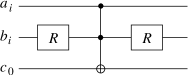
Figure 3.2: The operation $U$ on physical qubits $a_{i}\,b_{i}\,c_{0}$.

Apply $U$ bitwise over $a\,b$ and measure $Z_{c_{0}}$. The result $Z_{c_{0}}=\pm 1$ is equivalent to the result that $\dot{X}_{ab}=\prod_{i}\dot{X}_{a_{i}b_{i}}=\pm 1$, so one has effectively measured $\dot{X}_{ab}$. To understand this process in detail, expand the initial state of $a\,b$ in eigenstates of the operators $\dot{X}_{a_{i}b_{i}}$ for $i=1,\ldots,n$:

$$\sum_{\mathbf{x}}C_{\mathbf{x}}|\mathbf{x}\rangle=\left(\sum_{w(\mathbf{x})=0}+\sum_{w(\mathbf{x})=1}\right)C_{\mathbf{x}}|\mathbf{x}\rangle$$

where $|\mathbf{x}\rangle=|x_{1}\cdots x_{n}\rangle$ and each $|x_{i}\rangle$ is one of the four eigenstates ($x_{i}=1,2,3,4$) of $\dot{X}_{a_{i}b_{i}}$. The right hand sum is rearranged to segregate strings of even and odd weight. The weight function $w(\mathbf{x})$ equals the number (mod 2) of “4”s occurring in the string $\mathbf{x}$, $x_{i}=4$ corresponding to the $-1$ eigenstate $|10\rangle-|11\rangle$ of $\dot{X}_{a_{i}b_{i}}$. Using the transversality of C-NOT and the definition of $w(\mathbf{x})$, one finds $\dot{X}_{ab}|\mathbf{x}\rangle=(-1)^{w(\mathbf{x})}|\mathbf{x}\rangle$. Thus the sum over strings with $w(\mathbf{x})=0$ is the projection onto the $+1$ eigenspace of $\dot{X}_{ab}$, and the sum with $w(\mathbf{x})=1$ is the projection onto the $-1$ eigenspace. It follows that the action of $U=\prod_{i}U_{a_{i}b_{i}c_{0}}$ is

$$U|\mathbf{x}\rangle_{ab}|0\rangle_{c_{0}}=|\mathbf{x}\rangle_{ab}|w(\mathbf{x})\rangle_{c_{0}},$$

which means measuring $Z_{c_{0}}$ is equivalent to measuring $\dot{X}_{ab}$.

This method of measurement is highly sensitive to errors; just one physical bit error can change $w(\mathbf{x})$ for an entire string of bits, making the measurement result erroneous. As the block size $n$ gets large, the chances of an even number of such errors occurring becomes nearly equal to the chances of an odd number occurring. Thus the measurement result tells very little about whether a $+1$ eigenstate or a $-1$ eigenstate of $\dot{X}_{ab}$ has been obtained. This little bit of information, however, turns out to be important for preparing $|\psi_{2}\rangle$.

As mentioned the above procedure is fault-intolerant, since one physical bit phase error may infect $c_{0}$ and thus spread rampantly throughout the block. It can be made fault-tolerant by using an ancilla $c$, which is not just one bit, but a superposition of $n$ physical bits over all even weight strings (“weight” is now in the sense of counting “1”s). Such a superposition is prepared as

$$|\mathrm{even}\rangle_{c}=\left(\prod_{i}R_{c_{i}}\right)(|0\cdots 0\rangle_{c}+|1\cdots 1\rangle_{c}).$$

The gate $U_{a_{i}b_{i}c_{i}}$ will be applied bitwise across $a\,b\,c$ so that a single error in one block can at most spread to one bit in each of the other two blocks. Acting bitwise on $|x_{1}\rangle|\;\rangle_{c_{1}}$ through $|x_{n}\rangle|\;\rangle_{c_{n}}$, $U$ will flip a number of bits in the initial $c$ state equal (mod 2) to exactly $w(\mathbf{x})$. Thus

$$U|\mathbf{x}\rangle_{ab}|\mathrm{even}\rangle_{c}=\left\{\begin{array}[]{ll}|\mathbf{x}\rangle_{ab}|\mathrm{even}\rangle_{c}&w(\mathbf{x})=0\\ |\mathbf{x}\rangle_{ab}|\mathrm{odd}\rangle_{c}&w(\mathbf{x})=1\end{array}\right.$$ (3.5)

Measuring $Z_{c_{i}}$ bitwise over $c$ with the result $\prod_{i}Z_{c_{i}}=\pm 1$ is now equivalent to measuring $\dot{X}_{ab}$ with the result $\dot{X}_{ab}=\pm 1$. Note that a single phase error in the $n$-bit cat state, or equivalently a bit flip in the sum over even weight strings, will change this sum into one over odd weight strings, again altering the measurement result while still projecting the state onto one of the eigenspaces of $\dot{X}_{ab}$. So the measurement procedure is now fault-tolerant, but the measurement result is still highly sensitive to single bit errors, giving little information about which eigenspace the state $|\;\rangle_{ab}$ collapses into.

One can also perform a noisy measurement of the C-PHASE operator $\dot{Z}_{ab}$. The action of $\dot{Z}_{ab}$ is just to apply a minus sign if $a\,b$ are in $|11\rangle$, which is unitarily equivalent to $\dot{X}_{ab}$ through the basis change $R_{b}$. To measure $\dot{Z}_{ab}$ first apply $R_{b}$, then measure $\dot{X}_{ab}$ by the above method, and reapply $R_{b}$. These procedures may be adapted, by changing the bitwise operation $U$, to noisy measurement of such operators as $\dot{X}_{ab}\dot{X}_{cd}$, $\dot{Z}_{ab}\dot{Z}_{cd}$, and $\dot{Z}_{ab}\dot{Z}_{bc}$.

3.4 Preparing the Two-Qubit Mixed State

First prepare two logical qubits $a\,b$ as $(|0\rangle+|1\rangle)^{2}$ and measure $\dot{Z}_{ab}$ by the method given above, making use of an ancilla block $c$. If the measurement result were +1 and all qubits were error-free, one would have prepared exactly $|\psi_{2}\rangle$. But this will be changed by errors (i.e. decoherence, gate errors, or measurement errors) occurring either to the bits encoding $a$ and $b$ or to those of the cat-like ancilla $c$ used in the noisy measurement procedure. In fact $c$ is especially vulnerable because it is not protected by any code at all—a single bit error anywhere in $c$ can reverse the observed measurement result for $\dot{Z}_{ab}$.

Depending on whether errors are unitary or decoherent, this yields a cohererent or incoherent superposition of $|\psi_{2}\rangle$ and $|11\rangle$, which will be shown to be of the form $\rho(|\alpha_{3}|<1)$ in either the unitary or decoherent case, hence a candidate for purification.

Phase errors to the bits of $a\,b$ cannot be transmitted to $c$ by the above procedure, so are irrelevant. Bit flip errors to $a\,b$ can be transmitted but are equivalent to bit flip errors occurring to the bits of $c$ so all errors can be effectively regarded as occurring to $c$ alone. Let us first consider the case of (uncorrelated) errors purely decoherent in the Pauli basis $\sigma^{m}$, so that each qubit $c_{i}$ suffers no error, a phase error, a bit error, or both errors—each with some fixed classical probability.

Phase errors in $c$ can affect only the relative sign of terms in $|\mathrm{even}\rangle_{c}$ and $|\mathrm{odd}\rangle_{c}$ of (3.5), hence are extinguished once the $Z_{c_{i}}$ measurements are made. Depending on whether $c$ is attacked by an even or odd number of bit errors, the measured eigenvalue of $\dot{Z}_{ab}$ will be inferred either rightly or wrongly from the outcome of the $Z_{c_{i}}$ measurements. So given the result $\prod_{i}Z_{c_{i}}=+1$, an even number of bits errors will yield $|\psi_{2}\rangle$ as desired; however, an odd number will yield $|11\rangle$ unbeknownst to us.

If each $c_{i}$ suffers a bit error with probability $p_{i}$, the difference between the chances of an even number of bit errors and of an odd number is

$$\left(\prod_{i=1}^{n}\sum_{x_{i}=0,1}\right)(-1)^{x_{i}}p_{i}^{x_{i}}(1-p_{i})^{1-x_{i}}=\prod_{i}(1-2p_{i}).$$ (3.6)

Given that these two probabilities sum to 1, this implies the preparation procedure will yield not exactly $|\psi_{2}\rangle$, but the state $\rho(0,0,\alpha_{3})$ with

$$\alpha_{3}=\frac{1-\prod_{i}(1-2p_{i})}{1+\prod_{i}(1-2p_{i})}\approx 1-2\prod_{i}(1-2p_{i})$$

where the last expression holds for large $n$. It thus appears that one cannot tell whether or not $|\alpha_{3}|<1$ for a given ancilla block $c$ if even a few of its bits might have $p_{i}>1/2$. This is true even though current codes themselves are completely robust to these “defective” bits so long as their distribution is suitably uncorrelated and infrequent at the level of the code’s threshold error rate. Still what has to be considered for the purification process is not a single ancilla block $c$, giving rise to one $|\psi_{2}\rangle$-like state, but a sequence of such blocks, each with its own set of defective bits and consequent value of $\alpha_{3}=\alpha_{3}^{(m)}$, where $m$ runs from $1$ to $2^{N}$, the number of $|\psi_{2}\rangle$-like states input to the purification process.

The fidelity in purifying $|\psi_{2}\rangle$ is that given by (3.2) with $\alpha_{3}^{2^{N}}$ replaced by

$$\prod_{m}\alpha_{3}^{(m)}\approx e^{-2^{N+1}\left\langle\prod_{i}(1-2p_{i})\right\rangle},$$

where $\langle\cdots\rangle$ is an average over the ensemble of $c$ blocks. Assuming errors are uncorrelated between different $c$ blocks, the average factorizes and the purification fidelity is

$$1-{\textstyle\frac{1}{3}}\,e^{-2^{N+1}\prod_{i}(1-2\langle p_{i}\rangle)}.$$

Here only the ensemble averaged bit flip error rates appear. Assuming the locations of defective qubits are uncorrelated between different $c$ blocks, their $p_{i}>1/2$ contributions are simply weighted out in the average. This means infrequent defective bits no longer pose a problem, owing to the distributed nature of the purification process. Defining an average error rate $p=(1/n)\sum_{i}\langle p_{i}\rangle$, the above product is approximately $e^{-2pn}$. In order that the resulting fidelity be comparable to that of the code itself, which is $\sim 1-\exp(-Kn^{\beta})$ for some power $\beta$ and constant $K$, the number of physical qubits used in purification is roughly

$$n2^{N}\sim n^{1+\beta}e^{2pn},$$

which puts a limit on the block size $n$ of the code being used, since the number of qubits used in purification should not grow exponentially with block size. Thus $n$ cannot be larger than

$$n\sim\frac{1}{p}\log\frac{1}{p}.$$ (3.7)

The opposite case of purely unitary errors is the same in its result. Here, errors comprise a set of unitary operators which act on the $c_{j}$ respectively. Each such operator can be written in the Pauli basis and put in the form

$$E_{j}=(A_{j}\mathbf{1}+\mathrm{i}B_{j}\sigma^{z})+i\sigma^{x}(C_{j}\mathbf{1}+\mathrm{i}D_{j}\sigma^{z}),$$

where $A_{j},B_{j},C_{j},D_{j}$ are real. Assuming low error rates, so $\prod_{i}|A_{i}|\gg\prod_{i}|B_{i}|$ and likewise with $C_{i}$ and $D_{i}$ in place of $B_{i}$, one can show that these errors take $c$ from its prepared state $|\mathrm{even}\rangle$ to

$$\prod_{i}E_{i}|\mathrm{even}\rangle=|\mathrm{even}\rangle+\mathrm{i}\tan(\Sigma_{C})|\mathrm{odd}\rangle,$$

where $\Sigma_{C}\approx\sum_{i}\tan^{-1}(C_{i}/A_{i})$. This leads to preparation of the state $|\psi_{2}\rangle+\mathrm{i}\tan(\Sigma_{C})|11\rangle$ in place of $|\psi_{2}\rangle$. But this state is precisely $\rho(\alpha_{i})$ with $\alpha_{1,2}=\mathrm{i}\tan(\Sigma_{C})$ and $\alpha_{3}=-\tan^{2}(\Sigma_{C})$, which can be purified to $|\psi_{2}\rangle$ if $\tan^{2}(\Sigma_{C})<1$. For large $n$, $\Sigma_{C}$ will be very sensitive to the error amplitudes $C_{i}$, and in practice one would have no way of knowing whether $\tan(\Sigma_{C})<1$ or not. This is the same problem noted above in the case of pure decoherence, and it too disappears when one realizes that the purification input is not a single state $|\psi_{2}\rangle+\mathrm{i}\tan(\Sigma_{C})|11\rangle$ but an ensemble of such states each generated by a different set of blocks $a\,b\,c$. The purification fidelity is now given by (3.2) with $\alpha_{3}^{2^{N}}$ replaced by

$$\prod_{m=1}^{2^{N}}\tan^{2}(\Sigma_{C})\approx e^{2^{N+1}\langle\log(\tan\Sigma_{C})\rangle}.$$

where $\langle\cdots\rangle$ again averages over the ensemble of $c$ blocks. Using this, the definition of $\Sigma_{C}$, and expanding the logarithm gives $\langle\log(\tan\Sigma_{C})\rangle$ as

$$-\sum_{k=0}^{\infty}\frac{2}{2k+1}\prod_{i}\langle e^{-\mathrm{i}2(2k+1)\tan^{-1}(C_{i}/A_{i})}\rangle.$$ (3.8)

The factorization follows assuming independence of errors between different qubits in each $c$ block. Now expand the exponential in a power series. If the error distributions are all such that the two bit flip amplitudes $C_{i}$ and $-C_{i}$ are equally likely to occur, the expectation values of the odd terms in the power series vanish. (If the distributions are otherwise, one might use the computational basis $\{|0\rangle,-|1\rangle\}$ instead of $\{|0\rangle,|1\rangle\}$ for the qubits in half the $c$ blocks, so that the same physical error would correspond to the bit flip amplitude $-C_{i}$ as often as it would to $C_{i}$.) The even terms may then be resummed and the expectation value in (3.8) becomes

$$\left\langle\cos\left(2(2k+1)\tan^{-1}(C_{i}/A_{i})\right)\right\rangle\equiv\cos\left(2(2k+1)\sqrt{\langle p_{i}\rangle}\right),$$

where $\langle p_{i}\rangle=\langle C_{i}^{2}/A_{i}^{2}\rangle$ to lowest order in $C_{i}/A_{i}$, hence $\langle p_{i}\rangle$ can be taken roughly as a bit flip error rate. For small $k$ the cosine functions will be close to 1, and the product over $i$ will be greatest. As $k$ gets large, the cosines will sample their full range and the product will be highly suppressed. Therefore the cosine above can be replaced by $\exp(-2(2k+1)^{2}\langle p_{i}\rangle)$, as if $k$ were always small, giving the main contribution to the sum:

$$\langle\log(\tan\Sigma_{C})\rangle\;\sim\;-\sum_{k=0}^{\infty}\frac{2}{2k+1}e^{-2(2k+1)^{2}\sum_{i}\langle p_{i}\rangle}\;<\;{-2}e^{-2pn},$$

where $p$ is again the average of $\langle p_{i}\rangle$ over $i=1,\ldots,n$; this is basically the same result as obtained for purely decoherent errors. Thus again (3.7) gives the largest allowed block size in the regime where the resources needed for purification scale polynomially with block size.

3.5 Progressive Concatenation

In case higher fidelity is desired of the code than (3.7) allows, the above methods by themselves are insufficient and one must resort to concatenation. However, in conjunction with these methods, an unconventional, exponentially weaker form of concatenation can be used. A usual concatenated code is self- similar, the same abstract code (e.g. the 7-qubit code) being used at each level in its recursion. Here one is free to increase the block size at each level, as long as (3.7) is satisfied level-by- level. In these “progressive” concatenated codes, many fewer levels are necessary given a desired fidelity $1-\epsilon$.

In particular, for one error correction algorithm [22] in the context of lattice codes, some reasonable parameters are $p=p_{c}/10\lesssim 10^{-3}$, so that $n=1000$ is acceptable by (3.7). Here $\epsilon\sim(p/p_{c})^{n^{\beta}}$ where $\beta=\log_{9}2\approx.315$, which gives $\epsilon\sim 10^{-9}$. So, if the desired fideltiy is below $1-10^{-9}$, no concatenation is necessary. Otherwise, one can begin concatenating.

Consider a single concatenation of a chosen code. Physical qubits with error rate $\epsilon_{0}=p$ are arranged in code blocks of size $n_{1}$, and these blocks are themselves arranged in blocks of size $n_{2}$. The effective error rate at this higher level is just the failure rate of blocks at the lower level:

$$\epsilon_{1}\sim(\epsilon_{0}/p_{c})^{Kn_{1}^{\beta}},$$ (3.9)

where $p_{c}$, $K$, and $\beta$ come from details of the code being concatenated. The code as a whole has failure rate

$$\epsilon_{2}\sim(\epsilon_{1}^{\ast}/p_{c})^{Kn_{2}^{\beta}}.$$ (3.10)

where $\epsilon_{1}^{\ast}$ includes the effect of storage errors described by $\epsilon_{1}$ and also gate errors associated with the operations necessary to perform error correction. Thus $\epsilon_{1}^{\ast}$ will have the same form as $\epsilon_{1}$ in (3.9) but with $\epsilon_{0}=p$ replaced by a physical qubit error rate $\epsilon_{0}^{\ast}$ including the effect of these additional errors. In other words one must deal not only with a storage error threshold but also with a gate error threshold associated with the computations necessary for error correction. Of course, if one intends to use the logical qubits stored by the code for actual computations, this would be necessary anyway.

Assuming the effective error rate $\epsilon_{0}^{\ast}$ is still below threshold, a single concatenation of the code in the above example gives

$$\epsilon_{2}=\left(\frac{(\epsilon_{0}^{\ast}/p_{c})^{Kn_{1}^{\beta}}}{p_{c}}\right)^{Kn_{2}^{\beta}}\sim 10^{-830}$$

where the values $K=1$, $\beta=\log_{9}2$, and $\epsilon_{0}^{\ast}=p_{c}/5$ have been used. The block sizes $n_{1}=1000$ and $n_{2}=2\cdot 10^{7}$ were chosen to be consistent with $n_{L}\sim(1/\epsilon_{L-1}^{\ast})\log(1/\epsilon_{L-1}^{\ast})$, i.e. the condition (3.7) applied at each level. Thus, as long as one does not require a fidelity better than $1-10^{-830}$, a single concatenation is sufficient given the above parameters.

Because the block sizes $n_{L}$ may increase so rapidly, the number $N$ of levels necessary for a desired fidelity $1-\epsilon$ scales differently than in usual concatenation, in which $N\sim\log(\log(1/\epsilon))\equiv\log^{(2)}(1/\epsilon)$. For these progressive concatenated codes, $N$ is determined self-consistently by $N\sim\log^{(N)}(1/\epsilon)$. One might wonder about the asymptotic behavior of thresholds and fidelities as $N\rightarrow\infty$, taking into account the reciprocal effects between progressive concatenation and purification; however, this seems irrelevant given the smallness of $\epsilon$ already at $N=2$.

Chapter 4 Path Integrals and Beable Trajectories

The strategy employed in the last chapter to achieve a desired quantum state (in our case a certain two or three-qubit entangled state) by an iterative process of purification appears somewhat narrow in its application in the context of certain quantum error correcting codes. However it turns out this underlying idea can be translated into classical terms and proves valuable in defining a purely classical algorithm for the simulation of quantum systems—meaning, that the goal of the algorithm will be to simulate quantum systems but its implementation will be entirely concerned with classical computations on a normal computer.

As we have discussed, numerical simulation of quantum systems by classical algorithms is limited by the fact that the dimension of a system’s Hilbert space grows exponentially with the number of physical degrees of freedom. One general approach to this problem is to obtain a correspondence between the desired quantum system and a statistical ensemble of classical systems that are easier to simulate. Green function Monte Carlo [24] and coherent state representations in quantum optics [25] both derive Fokker-Planck equations, which can be realized through stochastic trajectories in an associated classical configuration space. Another category of methods well known in condensed matter and particle theory is that of path integrals with pseudo-dynamical importance sampling [26]. It turns out these configuration space methods are closely related to well known beable models of quantum mechanics.

Understanding these relationships offers another perspective on existing computational methods and also points the way to new such methods. In particular Monte Carlo, path integral, and coherent state representation approaches have mainly been applied by exploiting their connection to diffusion processes, with the result that calculations have been limited to ground state or thermal properties, or else very restricted classes of Hamiltonians. In the case of coherent state methods, like the $P$ or positive $P$ representation, Hamiltonians with higher than quadratic interaction terms give rise to master equations that cannot be cast as stochastic differential equations over an associated phase space. In the case of Monte Carlo and path integral methods, a connection to diffusion processes can only be made by going to imaginary time.

However, the beable methods to be presented here are naturally formulated in real time and are not restricted to narrow classes of Hamiltonians. Whatever their computational efficacy, they are thus at least well-defined, general methods for studying dynamics.

4.1 Langevin Method and Nelson’s Mechanics

The thermal expectation value of an operator $\mathcal{O}$ is often given in the form of an imaginary time path integral:

$$\langle\mathcal{O}\rangle=\int\mathcal{D}x\mathcal{O}(x)e^{-S_{\mathrm{E}}(x)}$$ (4.1)

where $S_{\mathrm{E}}(x)$ is some Euclidean action over the degrees of freedom $x=(x^{1},\ldots,x^{d})$. To compute this path integral we need a method to select paths over which the action may be sampled according to the weight $e^{-S_{\mathrm{E}}(x)}$. The methods to be considered here generate paths as the solutions of initial value problems in the classical configuration space $\{x\}$ of the system.

In the Langevin or “stochastic quantization” approach [26][27], $\langle\mathcal{O}\rangle$ is computed as a long-time average over a path $x(\tau)$ generated by the stochastic differential equation

$$dx^{i}=-\partial_{i}S_{\mathrm{E}}d\tau+\sqrt{2}dW^{i}$$ (4.2)

where $\hbar=1$, $\partial_{i}\equiv\partial/\partial x^{i}$, and $dW^{i}$ is a Wiener process, i.e. an independent Gaussian random variable at each $\tau$ with mean $\langle dW^{i}\rangle=0$ and variance $\langle(dW^{i})^{2}\rangle=d\tau$. Here, $\tau$ is not a time (real or imaginary) but an auxiliary variable introduced to parameterize paths. And one can show that an ensemble of trajectories evolving by (4.2) samples $e^{-S_{\mathrm{E}}(x)}$ in the limit $\tau\rightarrow\infty$

Nevertheless, observe the similarity between the Langevin equation (4.2) and the stochastic process involved in the generalized Nelson hidden variable theory [28] for particles of mass $m=1$ under a potential $V(x)$:

$$dx^{i}=\left(\partial_{i}S+\alpha\frac{\partial_{i}R}{R}\right)d\tau+\sqrt{\alpha}dW^{i}$$ (4.3)

where $dW^{i}$ is also a Wiener process, and $\alpha>0$ is a free parameter. Note that Nelson’s theory [29] results if $\alpha=1$ and Bohm’s deterministic theory [30] if $\alpha=0$. While (4.3) is normally defined in real time, we need the imaginary time analog for comparison with the path integral (4.1). This is easily obtained by taking $\psi(x,\tau)=Re^{S}$ as a solution of the imaginary time ($\tau=-it$) Schrodinger equation

$$\frac{\partial\psi}{\partial\tau}=-\frac{1}{2}\sum_{i}\partial_{i}^{2}\psi+V\psi$$ (4.4)

which will hold if we evolve $R$ and $S$ by

$$\frac{\partial R^{2}}{\partial\tau}+\sum_{i}\partial_{i}\left(R^{2}\partial_{i}S\right)=0$$ (4.5)

$$\frac{\partial S}{\partial\tau}+\frac{1}{2}\sum_{i}(\partial_{i}S)^{2}-V(x)-V_{\mathrm{q}}(x)=0$$ (4.6)

where

$$V_{\mathrm{q}}=-\frac{1}{2}\sum_{i}\frac{\partial_{i}^{2}R}{R}$$ (4.7)

is Bohm’s quantum potential.

The crux of this kind of hidden variable theory is that an ensemble of particles evolving by (4.3) will be distributed as $R(x,\tau)^{2}$ at time $\tau$ if they are initially distributed as $R(x,0)^{2}$ at time 0. This follows from the fact that the Fokker-Planck equation

$$\frac{\partial P}{\partial\tau}+\sum_{i}\partial_{i}\left[\left(\partial_{i}S+\alpha\frac{\partial_{i}R}{R}\right)P-\frac{\alpha}{2}\partial_{i}P\right]=0$$ (4.8)

for the distribution $P(x,\tau)$ generated by (4.3) becomes identical to the conservation equation (4.5) if we put $P=R^{2}$. Note that (4.5) and (4.8) are unchanged from the case of real time.

The effect of going to imaginary time is just to invert $V(x)$ and $V_{\mathrm{q}}(x)$ in (4.6), which resembles the classical Hamilton-Jacobi equation for the Euclidean action $S_{\mathrm{E}}=\int Hd\tau$, where $H$ is the classical Hamiltonian. In fact, (4.6) implies that $S=\int(H+V_{\mathrm{q}})d\tau$, where the integral is taken along a trajectory defined by the “current velocity” $v^{i}=\partial S/\partial x^{i}$, which means a Bohm trajectory.

Therefore, choosing $\alpha=2$ in (4.3) gives the time-reverse of the Langevin equation (4.2) except for extra $\psi$-dependent terms in the drift. The result is that, while the Langevin trajectories sample $e^{-S_{\mathrm{E}}(x)}$ in the limit $\tau\rightarrow\infty$, the Nelson trajectories generate a particle distribution that samples $R^{2}$ itself for all $\tau>0$. This suggests that we look for a Langevin-like method of importance sampling in which the drift is somehow guided by information we might have about $\psi(x,\tau)$.

4.2 Guided Random Walks

Indeed such a method already exists in the literature. It relies on a trial wavefunction $\psi$ to generate trajectories useful for the evaluation of observables, and these trajectories become exactly Nelson trajectories as $\psi$ becomes more accurate.

The ground state expectation value of some observable $\mathcal{O}$ is given by

$$\langle\mathcal{O}\rangle=\lim_{\tau\rightarrow\infty}\frac{\langle\psi_{0}|e^{-\tau H}\mathcal{O}\,e^{-\tau H}|\psi_{0}\rangle}{\langle\psi_{0}|e^{-2\tau H}|\psi_{0}\rangle}$$ (4.9)

where $|\psi_{0}\rangle$ is our trial evaluated at $\tau=0$. The exponential factors in the numerator serve to dampen out any excited state components in $\psi_{0}$ as $\tau\rightarrow\infty$. Identifying

$$\langle\psi_{0}|e^{-\tau H}|x\rangle=\bar{\psi}(x,\tau)$$

as a corresponding trial wavefunction for the imaginary time-reverse Schrodinger equation, (4.4) with $\tau\rightarrow-\tau$, and breaking the other $e^{-\tau H}$ factor into $N$ pieces $e^{-\epsilon H}\cdots e^{-\epsilon H}$, the numerator in (4.9) can be written as a path integral:

$$\int dx_{0}\cdots dx_{N}\,\bar{\psi}(x_{0},0)\psi(x_{0},0)\mathcal{O}(x_{N})\prod_{p=0}^{N-1}U_{\epsilon}(x_{p+1},x_{p})$$ (4.10)

$$U_{\epsilon}(x_{p+1},x_{p})\equiv\langle x_{p+1}|e^{-\epsilon H}|x_{p}\rangle\frac{\bar{\psi}(x_{p+1},\tau_{p+1})}{\bar{\psi}(x_{p},\tau_{p})}$$ (4.11)

where $x_{p}=(x_{p}^{0},\ldots,x_{p}^{d})$ denotes a single classical configuration of the system at time $\tau_{p}=p\epsilon$, and we have assumed that $\mathcal{O}$ is a local observable with matrix elements $\langle x|\mathcal{O}|x^{\prime}\rangle=\delta(x-x^{\prime})\mathcal{O}(x)$. The ratio of $\bar{\psi}$ terms in (4.11) produces a sequence of cancellations that allows us to have $\bar{\psi}$ evaluated at $\tau=0$ in (4.10). To lowest order in $\epsilon$, it can be shown [31] that

$$U_{\epsilon}(x_{p+1},x_{p})=(2\pi\epsilon)^{-\frac{d}{2}}\;e^{-\sum_{i}\frac{1}{2\epsilon}\left(x_{p+1}^{i}-x_{p}^{i}-D_{p}^{i}\right)^{2}}e^{-\Delta S_{p}}$$ (4.12)

where the drift and residual action are given by

$$D_{p}^{i}=\epsilon\left[\frac{\partial}{\partial x^{i}}\log\bar{\psi}\right]_{x_{p}}$$ (4.13)

$$\Delta S_{p}=\epsilon\left[H\bar{\psi}-\frac{\partial}{\partial\tau}\bar{\psi}\right]_{x_{p}}\,.$$

In the method of guided random walks [26], the path integral (4.10) is sampled by stochastic trajectories over configuration space $\{x\}$. In particular, the Gaussian factor in (4.12) is interpreted as the probability to go from $x_{p}$ to $x_{p+1}$ over the $p$-th time step, and $e^{-\sum_{p}\Delta S_{p}}$ gives the “score” of the path $(x_{0},\ldots,x_{N})$ in the stochastic average.

Now, if $\bar{\psi}(x,\tau)$ were chosen to exactly satisfy the time-reverse Schrodinger equation, we see that $\Delta S_{p}$ would vanish and the trajectories would optimally sample (4.10). But then, as $\epsilon\rightarrow 0$, the jump probability in (4.12) and the drift (4.13) exactly match those of Nelson’s theory, (4.3) with $\alpha=1$. In other words, the guided random walk method of importance sampling can be seen as an attempt to generate Nelson trajectories (for the time-reverse problem) with a trial wavefunction defining the drift.

The fact that the generalized Nelson theory (4.3) matches the quantum evolution for any $\alpha>0$ suggests a new one-parameter family of guided random walk algorithms for path integral evaluation, with $\alpha$ controlling the strengths of both the diffusion and the drift. This family is similar to the family of hybrid Langevin molecular dynamics algorithms introduced by Kogut and Duane [32], with the pure molecular dynamics algorithm in the Kogut family corresponding to Bohm trajectories ($\alpha=0$) in our family. While both of these last algorithms are deterministic, there does not appear to be any quantitative relationship between them.

4.3 Iterated Bohm Trajectories

The effectiveness of importance sampling in a guided random walk algorithm depends on the accuracy of the trial wavefunction. It would therefore be desirable if one could use information gained from the trajectories themselves to improve the trial and generate new trajectories. Iterating the process may then produce a sequence $(\psi^{(0)},\psi^{(1)},\ldots)$ of successively better trial wavefunctions.

The following method in the case of pure Bohm trajectories is due to Goldstein [33]. Since Bohm’s theory is equally applicable to real time $t$, let us return to that case. Bohm’s equations of motion, obtained by using (4.3) with $\alpha=0$ and differentiating the real time version of (4.6) are

$$\frac{d}{dt}v^{i}=-\frac{\partial}{\partial x^{i}}\left[V(x)+V_{\mathrm{q}}(x,t)\right]$$ (4.14)

with the minus sign replaced by a plus sign in the imaginary time case of (4.4). Here the Bohm particle velocity $v^{i}$ is identified with $\partial S/\partial x^{i}$ as usual in Hamilton-Jacobi theory, except that this $S$, from (4.6), includes the effect of $V_{\mathrm{q}}$ in addition to the classical potential $V$. Also, here,

$$\frac{d}{dt}=\frac{\partial}{\partial t}+\sum_{i}v^{i}\frac{\partial}{\partial x^{i}}$$

defines the the convective or “along-the-trajectory” derivative.

Writing $\psi^{(0)}=R^{(0)}e^{\mathrm{i}S^{(0)}}$, we evolve trajectories according to (4.14) with $R^{(0)}$ used to the calculate $V_{\mathrm{q}}$ in (4.7). Were $\psi^{(0)}$ an exact solution, (4.5) and (4.6) would ensure that these trajectories generate a particle distribution equal to $(R^{(0)})^{2}$. However, with an inexact trial wavefunction, the actual distribution will differ from $(R^{(0)})^{2}$. We can thus use this actual distribution to define the next iterate $R^{(1)}$, which can then be used to obtain a new $V_{\mathrm{q}}$, new trajectories from (4.14), and a new phase $S^{(1)}$ if desired. Iterating this procedure yields a sequence $(\psi^{(0)},\psi^{(1)},\ldots)$ that has the exact solution $\psi$ as a fixed point; however, convergence is not guaranteed for any fixed number of trajectories being propagated.

There is also another technical issue. The equations of motion (4.14) will generate unique non-crossing trajectories when $V_{\mathrm{q}}$ is obtained exactly from $\psi(x,t)$, but no such guarantee exists for an inexact iterate $\psi^{(i)}$. Viewing (4.14), with $\psi^{(i)}$ used to calculate $V_{\mathrm{q}}$, as defining a map from configuration space at time $0$ to itself at time $t$, one thus finds that the map will generically be many-to-one. In effect, for $t$ large enough, $\psi^{(i)}(x,t)$ would be a multivalued function of $x$. Either dealing with this multivalued-ness or eliminating it by fiat poses a significant problem in defining the algorithm.

Goldstein’s iterative algorithm can also be compared to moving grid methods for quantum dynamics that rely on Bohm trajectories to define the grid [34] [35]. These methods propagate a swarm of Bohm trajectories similar to the way a fluid dynamics algorithm propagates a large number of fluid elements, and therefore they do not require any trial wavefunction to get started. They are PDE propagator algorithms that are truly local in time and (configuration) space.

4.4 Discrete Beables

Let us now consider methods posed explicitly for a finite dimensional Hilbert space spanned by the basis states $|n\rangle$ with $n=1,\ldots,N$ and with Schrodinger equation

$$\frac{d}{dt}|\psi(t)\rangle=-\mathrm{i}H|\psi(t)\rangle\,.$$ (4.15)

Originally for the purpose of attacking conceptual problems in quantum field theory, John Bell found an analog of Bohm’s model in which trajectories are generated by “beables” (i.e. classical-like particles in state space) stochastically jumping between states connected by non-zero Hamiltonian matrix elements [36]. In place of (4.3), Bell takes the probability for a trajectory to jump from state $m$ to a distinct state $n$, sometime in the interval $(t,t+\epsilon)$, as

$$T_{nm}(t)\,\epsilon=\left\{\begin{array}[]{ll}2\,\mathrm{Re}\{z_{nm}(t)\}\,\epsilon&\mbox{if Re$\{z_{nm}(t)\}>0$}\\ 0&\mbox{if Re$\{z_{nm}(t)\}\leq 0$}\end{array}\right.$$ (4.16)

where we define

$$z_{nm}(t)=-\mathrm{i}H_{nm}\frac{\psi_{n}(t)^{\ast}}{\psi_{m}(t)^{\ast}}\,.$$ (4.17)

and $\psi_{n}=\langle n|\psi\rangle$, etc. To ensure normalization, the probability for a trajectory to stay at $m$ is thus given by $1-\sum_{n}^{\prime}T_{nm}(t)\epsilon$, where the primed sum excludes the diagonal term $n=m$. Note the similarity between (4.17) and (4.11). But here jumping from $m$ to $n$ is allowed only if there is a non-zero matrix element $H_{nm}$ for the transition.

From (4.17), we find

$$\mathrm{Re}\{z_{nm}\}=-\mathrm{Re}\{z_{mn}\}\frac{|\psi_{n}|^{2}}{|\psi_{m}|^{2}}\,,$$ (4.18)

which implies that either $T_{nm}=0$ or $T_{mn}=0$. Together with (4.15) this gives

$$\frac{d}{dt}|\psi_{n}|^{2}=\sum_{m}2\,\mbox{Re}\{z_{nm}|\psi_{m}|^{2}\}=\sum_{m}(T_{nm}|\psi_{m}|^{2}-T_{mn}|\psi_{n}|^{2})$$ (4.19)

in analogy with (4.5). Note that the $T_{nm}$ term contributes when Re$\{z_{nm}\}>0$, and the $T_{mn}$ term contributes when Re$\{z_{nm}\}<0$.

Now consider the distribution $P_{n}(t)$ of beables in state space, jumping in accordance with (4.16). The analog of the Fokker-Planck equation (4.8) is

$$\frac{d}{dt}P_{n}=\sum_{m}(T_{nm}P_{m}-T_{mn}P_{n})\,.$$ (4.20)

And this becomes identical to (4.19) if we put $P_{n}=|\psi_{n}|^{2}$. Thus, provided $P_{n}(0)=|\psi_{n}(0)|^{2}$, we are guaranteed $P_{n}(t)=|\psi_{n}(t)|^{2}$ for all $t>0$, just as in the continuous case.

4.5 A New Guided Random Walk

Can we find a stochastic method for path integral evaluation resembling Bell trajectories? Consider the real-time analog of (4.10) for a finite dimensional Hilbert space, so that the continuous variables $x_{p}$ are replaced by discrete ones $n_{p}$. We can make a connection to Bell’s theory by expanding $e^{-\mathrm{i}\epsilon H}$ to first order in $\epsilon$ and evaluating matrix elements. Assuming a diagonal observable $\langle n|\mathcal{O}|m\rangle=\delta_{nm}\mathcal{O}_{n}$, we get

$$\langle\mathcal{O}\rangle_{t}=\sum_{\mathcal{P}(N)}\psi_{n_{N}}(t)^{\ast}\psi_{n_{0}}(0)\,\mathcal{O}_{n_{N}}\prod_{p\in J}(-\mathrm{i}\epsilon H_{n_{p+1}n_{p}})$$ (4.21)

where $\mathcal{P}(N)=(n_{0},\ldots,n_{N})$ specifies a path in which $H_{n_{p+1}n_{p}}\neq 0$ for each $n_{p+1}\neq n_{p}$. The jump set is defined as $J[\mathcal{P}]=\{p\;|\;n_{p+1}\neq n_{p}\}$. Now we can use the same trick of introducing $\psi$ ratios to write

$$\psi_{n_{N}}(t)^{\ast}\prod_{p\in J}(-\mathrm{i}H_{n_{p+1}n_{p}})=\psi_{n_{0}}(0)^{\ast}\prod_{p\in J}z_{n_{p+1}n_{p}}(t_{p})\prod_{p\notin J}\frac{\psi_{n_{p}}(t_{p+1})^{\ast}}{\psi_{n_{p}}(t_{p})^{\ast}}$$ (4.22)

with $z_{nm}$ as in (4.17).

To realize (4.21) as a weighted average over stochastic processes, we need to choose the jump rates $T_{nm}$ so that the probability

$$\mathrm{Prob}[\mathcal{P}(N)]=\prod_{p\in J}\epsilon T_{n_{p+1}n_{p}}\prod_{p\notin J}(1-\epsilon{\textstyle\sum_{n}^{\prime}}T_{nn_{p}})$$ (4.23)

of realizing a given path $\mathcal{P}(N)$ resembles the double product in (4.22) as closely as possible. $\sum_{n}^{\prime}$ is a sum excluding the diagonal term ($n=n_{p}$ here).

Consider the choice would be ($n_{p+1}\neq n_{p}$):

$$T_{n_{p+1}n_{p}}=|z_{n_{p+1}n_{p}}|a_{p}$$ (4.24)

where the $z_{nm}$ are given by (4.17) with our trial wavefunction $\psi$, and the $a_{p}$ are to be determined. The remaining phase factors in (4.22) not assimilated into (4.23) will then constitute the complex “score” of the path $\mathcal{P}(N)$ in the stochastic average. That is, the stochastic average that computes (4.21) is obtained by propagating trajectories according to (4.24), calculating the score of each trajectory, and adding up all the scores.

One can show that apart from endpoint contributions around $p=0,N$, the double products are matched in absolute value with error O$(N\epsilon^{2})$ if the $a_{p}$ satisfy

$$\sum_{p}\left(\frac{\log a_{j(p)}}{N_{p}\epsilon}-a_{p}{\textstyle\sum_{n}^{\prime}}|z_{nn_{p}}|-\frac{\partial}{\partial t}\log|\psi_{n_{p}}(t_{p})|\right)=0$$ (4.25)

where $j(p)$ is the largest member of $J$ less than $p$, and $N_{p}$ is the number of time steps between the $j(p)$-th step and the next jump. Unfortunately we cannot make the sum vanish term by term. When we need to choose $a_{p}$ at the $p$-th time step, we do not yet know the value of $N_{p}$ for the trajectory, because we do not yet know when the next jump will occur. It is therefore necessary to choose $a_{p}$ dynamically. At each time step $p$ we can evaluate the sum (4.25) up to $p$ and choose $a_{p}$ to stabilize it back toward 0.

In particular, if we change $a_{p}$ only just after a jump, so that $a_{p}=a_{j(p)+1}$ for all $p$, we can explicitly calculate the expectation value of the sum (4.25) with respect to variations in $N_{p}$ produced by the the jump probabilities (4.24). Setting this expectation value to zero, term by term, and solving for $a_{p}$ yields a critical value such that choosing $a_{p}$ above (below) the critical value will tend over time to increase (decrease) the sum. This enables us to stabilize the sum and achieve a correspondence between, on the one hand, a stochastic average over trajectories defined by (4.24) and, on the other hand, the path sum (4.21).

We have thus obtained a stochastic algorithm for evaluation of the discrete path integral that resembles Bell’s discrete hidden variable theory. As opposed to the standard random walk algorithms, this one involves trajectories that jump from one site to another only if there is a non-zero matrix element for the transition. In particular, with a spatial basis $|n\rangle$ and a local Hamiltonian, the path space is reduced considerably. The price is that the trajectory scores become complex in the case of imaginary time as well as in real time.

If the matrix elements $H_{nm}$ are bounded and independent of $t$, a generic estimate may be obtained for the importance of different classes of paths. Going back to (4.21) and performing the sum over paths comprising the same sequence of jumps, differing only by when each jump occurs, we have

$$\langle\mathcal{O}\rangle_{t}=\sum_{M=0}^{N}\mathcal{O}_{n_{M}}\left(\begin{array}[]{@{}c@{}}N\\ M\end{array}\right)\zeta_{M}[\psi]$$ (4.26)

$$\zeta_{M}[\psi]\equiv\sum_{\bar{\mathcal{P}}(M)}\psi_{n_{M}}^{\ast}\psi_{n_{0}}\prod_{p=0}^{M-1}(-\mathrm{i}\epsilon H_{n_{p+1}n_{p}})\,.$$ (4.27)

$\zeta_{M}$ is a kind of partition function summing over all paths $\bar{\mathcal{P}}(M)=(n_{0},\ldots,n_{M})$ without stops: $n_{p+1}\neq n_{p}$ for all $p=0,\ldots,M-1$. The binomial coefficient counts the number of paths $\mathcal{P}(N)$ from (4.21) that correspond to one path $\bar{\mathcal{P}}(M)$ in (4.26).

Using Stirling’s formula, (4.26) may be approximated as

$$\langle\mathcal{O}\rangle_{t}=\sum_{M}\mathcal{O}_{n_{M}}e^{S(M)}$$ (4.28)

$$S(M)=M\log\left(\frac{eN}{M}\right)-\frac{M^{2}}{N}+\log\zeta_{M}\,.$$ (4.29)

Now, $\log|\zeta_{M}|\sim M\log\epsilon$ can be interpolated into a smooth function of $M$ for any finite $\epsilon$. However, from (4.27) we can write

$$\zeta_{M+1}=\sum_{\bar{\mathcal{P}}(M)}\psi_{n_{M}}^{\ast}\phi_{n_{0}}\prod_{p=0}^{M-1}(-\mathrm{i}\epsilon H_{n_{p+1}n_{p}})\left[{\textstyle\sum_{n}^{\prime}}(-\mathrm{i}\epsilon H_{nn_{M}})\frac{\psi_{n}^{\ast}}{\psi_{n_{M}}^{\ast}}\right]\,,$$ (4.30)

which means that $\zeta_{M+1}$ is obtained from $\zeta_{M}$ by multiplying each term in the path sum by a different factor with magnitude O$(\epsilon)$ and unconstrained phase. This suggests that $\arg(\zeta_{M+1})$ will differ randomly from $\arg(\zeta_{M})$, so that $\mathrm{Im}(\log\zeta_{M})=\arg(\zeta_{M})$ can not be interpolated into a smooth function of $M$. Thus we expect $\mathrm{Re}\{S\}$, not $\mathrm{Im}\{S\}$, to control which terms are dominant in (4.28).

To find these terms we need to evaluate

$$\frac{d}{dM}\mathrm{Re}\{S\}=\log\left(\frac{N}{M}\right)-\frac{2M}{N}+\frac{d}{dM}\log|\zeta_{M}|\,.$$

Care must be taken in defining the derivative on the right, since $\log|\zeta_{M}|$ diverges as $\epsilon\rightarrow 0$. We use the finite difference

$$\frac{d}{dM}\log|\zeta_{M}|\;\approx\;\log|\zeta_{M+1}|-\log|\zeta_{M}|$$

together with (4.30) and the definition (4.17) to get

$$\frac{d}{dM}\log|\zeta_{M}|\;\approx\;\log\left(\epsilon\left|\left\langle{\textstyle\sum_{n}^{\prime}}z_{nn_{M}}\right\rangle_{M}\right|\right)$$

where $\langle\cdots\rangle_{M}$ averages over all paths $\bar{\mathcal{P}}(M)$ with complex weight as in (4.27).

Solving the saddle point equation $dS/dM=0$ will determine which path lengths $M$ are most important for computing (4.26). This equation has the form

$$\log x+2x+A=0$$

where $A\rightarrow\infty$ as $\epsilon\rightarrow 0$, and one can verify that

$$x=e^{-A-2e^{-A-2e^{-A-\cdots}}}$$

is an explicit solution. When $A$ is large, $x=e^{-A}$ is a very good approximation, which gives the saddle point equation

$$M=t\left|\left\langle{\textstyle\sum_{n}^{\prime}}z_{nn_{M}}\right\rangle_{M}\right|\,,$$ (4.31)

whose solution we denote $M=M_{\ast}$. Note that the right side of (4.31) itself depends on $M$. However, assuming $H_{nm}$ are bounded, ${\textstyle\sum_{n}^{\prime}}\langle z_{nn_{M}}\rangle_{M}$ will be bounded, and the solution $M_{\ast}$ will not be very sensitive to its $M$-dependence.

To determine the spread of dominant terms around $M=M_{\ast}$, we evaluate

$$\frac{d^{2}}{dM^{2}}\mathrm{Re}\{S\}=-\frac{1}{M}-\frac{2}{N}+\frac{d^{2}}{dM^{2}}\log|\zeta_{M}|$$ (4.32)

by putting

$$\frac{d^{2}}{dM^{2}}\log|\zeta_{M}| \approx \log|\zeta_{M+2}|-2\log|\zeta_{M+1}|+\log|\zeta_{M}|$$

$$= \log\left(\frac{|\zeta_{M+2}/\zeta_{M}|}{|\zeta_{M+1}/\zeta_{M}|^{2}}\right)\,.$$

Separating out two extra matrix elements of $H$ in $\zeta_{M+2}$ as we had separated out one matrix element in (4.30), we obtain

$$\frac{d^{2}}{dM^{2}}\log|\zeta_{M}|\;\approx\;\log\left(\frac{\left|\left\langle{\textstyle\sum_{mn}^{\prime}}z_{mn}z_{nn_{M}}\right\rangle_{M}\right|}{\left|\left\langle{\textstyle\sum_{n}^{\prime}}z_{nn_{M}}\right\rangle_{M}\right|^{2}}\right)$$ (4.33)

which is independent of $\epsilon$. If this term dominates in (4.32), it will control the spread of terms around $M=M_{\ast}$ that contribute to (4.28). Otherwise, $1/M_{\ast}$ will set the scale of (4.32), and the spread will be $\Delta M\sim\sqrt{M_{\ast}}$.

Consider a simple limiting case where the diagonal matrix elements $H_{nn}=E_{0}$ are all equal, and we choose $|\psi\rangle$ in (4.26) such that $H|\psi\rangle=E|\psi\rangle$. Now it is easy to verify that ${\textstyle\sum_{n}^{\prime}}z_{nm}=E-E_{0}$ for any $m$, so that (4.31) gives $M_{\ast}=|E-E_{0}|t$. Also, (4.33) vanishes, leaving the spread as $\Delta M\sim(|E-E_{0}|t)^{1/2}$.

4.6 Iterated Bell Trajectories

While we have succeeded in re-analyzing the path sum in a way motivated by Bell’s jump rule (4.16), the new rule (4.24) is somewhat cumbersome to implement and gives rise to complex path scores. A more natural approach is found by going the other way: re-analyzing Bell’s jump rule in a way motivated by path integral methods.

Consider the observable $\mathcal{O}=|n\rangle\langle n|$, so that $\langle\mathcal{O}\rangle_{t}=|\psi_{n}(t)|^{2}$. (4.21) now gives the path integral representation of a kind of Green function for $|\psi_{n}(t)|^{2}$ rather than $\psi_{n}(t)$. The classical analog of this in probability theory is just the equation

$$P_{n}(t)=\sum_{\mathcal{P}(N-1)}P_{n_{0}}(0)\,\mathrm{Prob}[\mathcal{P}(N)]$$ (4.34)

where the sum is taken over all paths $\mathcal{P}(N)$ with $n_{N}=n$ fixed. This gives the expectation value of a classical state function $\mathcal{O}$ as

$$\langle\mathcal{O}\rangle_{t}=\sum_{\mathcal{P}(N)}\mathcal{O}_{n_{N}}P_{n_{0}}(0)\,\mathrm{Prob}[\mathcal{P}(N)]\,.$$ (4.35)

What makes this merely an analogy to the quantum case is that in the latter the amplitudes involved in the path sum are generally complex, seemingly a necessity to achieve the affects of quantum interference. But Bell has shown us that we need not be content with just an analogy. The integral formulation of Bell’s model based on (4.23) re-expresses the quantum path sum with a real, strictly positive path amplitude, exactly as in (4.34) and (4.35). This is accomplished simply by choosing the $T_{nm}$ according to (4.16), with the result that $P_{n}(t)=|\psi_{n}(t)|^{2}$ for all $t>0$ if we set $P_{n}(0)=|\psi_{n}(0)|^{2}$. Quantum interference effects, here, are not manifested by the contributions from certain paths cancelling those from other paths, but rather by the propensity of beable trajectories to follow or not to follow certain paths in the first place. The sum over histories is manifestly undemocratic here.

To implement this as a stochastic algorithm we need to use a trial wavefunction for $\psi$ in (4.17). The beable distribution $P_{n}(t)$ of the resulting trajectories then serves to compute $|\psi_{n}(t)|^{2}$ and $\langle\mathcal{O}\rangle_{t}$ as stochastic averages for (4.34) and (4.35) respectively.

In analogy with Goldstein’s algorithm, we might then attempt to use these trajectories to generate a new trial $\psi^{(1)}$, which could be used to generate new trajectories, etc. The problem is that, while in the continuous case knowledge of $P^{(i)}=|\psi^{(i)}|^{2}$ is enough to compute new trajectories via (4.14), here we need $\mathrm{Re}\{z^{(i)}\}$ to compute new trajectories via (4.16). But $\mathrm{Re}\{z^{(i)}\}$ depends on the phase as well as the amplitude of $\psi^{(i)}$.

What must be done is to derive an evolution equation for $\mathrm{Re}\{z_{nm}\}$ from (4.15) in the discrete case, just as Bohm obtained (4.14) from the continuous Schrodinger equation. Using (4.15) to differentiate the definition (4.17) gives

$$\frac{d}{dt}z_{nm}=z_{nm}\sum_{k}(z_{km}-z_{kn})$$ (4.36)

which contains the same information as (4.15) itself. Notice that the (time-independent) Hamiltonian does not enter as a parameter in this equation, but only in the initial conditions when the $z_{nm}(0)$ are given in terms of the $\psi_{n}(0)$. An additional $dH/dt$ term would appear in (4.36) for the time-dependent case.

Now consider propagating (4.36) along a trajectory $\mathcal{P}$ at the $i$-th stage of iteration. One scheme would be to evolve $z_{n_{p+1}n_{p}}^{(i)}$ along $\mathcal{P}$ by evaluating the right hand side of (4.36) with $z^{(i-1)}$. But we might as well take the $z_{nm}$ factor on the right hand side as the current iterate $z^{(i)}$, since we can do so with the information obtained just from propagating $\mathcal{P}$. Thus we propagate

$$\frac{d}{dt}z_{nm}^{(i)}=z_{nm}^{(i)}\sum_{k}(z_{km}^{(i-1)}-z_{kn}^{(i-1)})$$ (4.37)

along beable trajectories generated by the jump rule $T_{nm}^{(i)}=2\mathrm{Re}\{z_{nm}^{(i-1)}\}$ ($\mathrm{Re}\{z\}>0$). An alternative scheme can be obtained by defining

$$Z_{m}\equiv\sum_{n}z_{nm}=\sum_{n}-\mathrm{i}H_{nm}\frac{\psi_{n}(t)^{\ast}}{\psi_{m}(t)^{\ast}}=-\frac{d}{dt}\log\psi_{m}^{\ast}(t)$$ (4.38)

and summing (4.36) over $n$, which gives

$$\frac{d}{dt}Z_{m}=Z_{m}^{2}-\sum_{n}Z_{n}\,z_{nm}\,.$$ (4.39)

Using (4.38) in (4.36), we obtain the time-dependence $z_{nm}\propto\exp[\int(Z_{m}-Z_{n})dt]$ and can thus eliminate the $z_{nm}$ from (4.39). After extracting the $n=m$ term from the sum, we have

$$\frac{d}{dt}Z_{m}=Z_{m}^{2}+\mathrm{i}H_{mm}Z_{m}-\sum_{n(\neq m)}Z_{n}\,z_{nm}(0)\exp\left(\int_{0}^{t}\left[Z_{m}(s)-Z_{n}(s)\right]ds\right)$$ (4.40)

as a replacement for (4.36). This can be cast for an iteration scheme by taking the $Z$’s in the sum as $(i-1)$-th iterates, hence known functions in the above equation, and the other $Z$’s as $i$-th iterates. It would also be possible to keep $Z_{m}$ in the sum as an $i$-th iterate, but this would result in a complicated integro-differential equation.

Having propagated the $i$-th ensemble of trajectories and calculated $Z^{(i)}$—$z^{(i)}$ in the former scheme—along each of them, we still have to determine $Z^{(i)}$ for the sites in state space that neither contain or neighbor any members of the beable ensemble at each time step. The natural choice in the present context of a discrete state space is simply to retain the $Z^{(i-1)}$ values at these sites. Since trajectories are attracted to sites with large $|\psi^{(i)}|^{2}$, this will cause the algorithm to concentrate on these sites and not on the low probability ones.

In essence, this scheme is constructed so that the iterate $Z^{(i-1)}$ guides the $i$-th set of trajectories, which then serve as an importance sampling prescription to calculate the next iterate $Z^{(i)}$. In this way an initial trial $Z^{(0)}$, or equivalently $\psi^{(0)}$, may be iteratively improved as the algorithm (hopefully) converges in computing the dynamical expectation value $\langle\mathcal{O}\rangle_{t}$ for a given observable $\mathcal{O}$.

The effectiveness of this method of importance sampling, here in the context of sampling entire dynamical evolutions as opposed to simply ground state distributions, is a delicate matter above and beyond questions of the stability and accuracy of the iteration scheme itself.

In implementing this algorithm, one must be cautious of potential divergences of the $Z_{m}$, since this will generally occur if $\psi_{m}=0$. Fortunately, we will not have to control these divergences in a very sensitive manner when solving the dynamical equations (4.40) themselves because we expect successive iterates to iron out any initial imperfections. Our goal is then merely to prevent catastrophic events that might corrupt computations occuring on neighboring sites. We can accomplish this much with a simple implicit method (supressing the site index):

$$Z(t+\Delta t)=Z(t)+Z^{\prime}(t)\Delta t+\mathrm{O}(\Delta t^{2})=\frac{Z(t)}{1-\frac{Z^{\prime}(t)}{Z(t)}\Delta t}+\mathrm{O}(\Delta t^{2})\,.$$

In fact, for better accuracy, we adopt a second order implicit method based on the relation:

$$Z(t+\Delta t)=\frac{Z(t)}{1-\frac{Z^{\prime}(t)}{Z(t)}\Delta t+\left(\frac{Z^{\prime}(t)^{2}}{Z(t)^{2}}-\frac{1}{2}\frac{Z^{\prime\prime}(t)}{Z(t)}\right)\Delta t^{2}}+\mathrm{O}(\Delta t^{3})\,.$$

The form of the denominator has been chosen to reproduce the appropriate Taylor expansion up to second order and requires a computation of $Z^{\prime\prime}(t)$, which can be accomplished by differentiating (4.40) once to get

$$\frac{d^{2}}{dt^{2}}Z_{m}=(2Z_{m}+\mathrm{i}H_{mm})\frac{dZ_{m}}{dt}-\sum_{n(\neq m)}Z_{n}\,z_{nm}\left[\frac{dZ_{n}}{dt}+Z_{n}(Z_{m}-Z_{n})\right]\,.$$

To implement this in our iteration scheme, we must remember that terms in the sum are to be taken as $(i-1)$-th iterates and terms outside the sum as $i$-th iterates.

In order to propagate (4.40) along trajectories we need to compute both $Z$ and $\int Zdt$ at each step. The latter must also be done to second order by expanding the integrand in $\int_{t}^{t+\Delta t}Z(s)ds$ around $s=t$:

$$\int_{t}^{t+\Delta t}\left[Z(t)+Z^{\prime}(t)(s-t)+\cdots\right]ds=Z(t)\Delta t+{\textstyle\frac{1}{2}}Z^{\prime}(t)\Delta t^{2}+\mathrm{O}(\Delta t^{3})\,.$$

There is nothing in principle to prohibit an implicit third or higher order method for propagating $Z$ and $\int Zdt$ along these lines; each higher order would simply require another differentiation of (4.40).

The distinguishing characteristic of an iterative algorithm such as the one presented here is that while the solution $Z$ at some time $t$ will be directly fixed in any one iteration by $Z$ at times just prior to $t$, successive iterates will bring in information from much further back before $t$. The global nature of this process is paid for by the computational cost of propagating a whole new time-development for each iterate.

However, it is possible to taylor this trade-off by subdividing the total simulation interval $(0,T)$ into windows $(t_{w-1},t_{w})$ each of some fixed duration $\Delta t_{W}$ so that iteration will proceed in each window until convergence is obtained before moving on to the next window. Thus, in the first window, the initial conditions $Z(t=0)$, together with some initial guess for $Z(0<t<t_{1})$, will be used to begin iteration, and after convergence is reached the solution endpoint $Z(t_{1})$ will provide the initial condition for the next sequence of iterations over $(t_{1},t_{2})$, etc.. We will determine that convergence has been reached by the $i$-th iterate in a given window $(t_{w-1},t_{w})$, if the correlation coefficient of the two data sets $\{Z_{m}^{(i-1)}(t_{w})\}$ and $\{Z_{m}^{(i)}(t_{w})\}$ exceeds some threshold value very close to 1.

As with the guided random walk methds, we also need some kind of trial wavefunction—here, as the initial iterate $\psi^{(0)}(t)$ or $Z^{(0)}(t)$ for each window $(t_{w-1},t_{w})$. One may obtain this $\psi^{(0)}$ from a completely separate method, which would likely rely on considerations more specific to the Hamiltonian in question. However, in order to concentrate on the iterative algorithm alone, we will use a rather simple trial:

$$Z^{(0)}(t)=Z^{(f)}(t_{w-1})\;\;\;t\in(t_{w-1},t_{w})$$ (4.41)

where $f$ indicates the final iteration of the previous window. The benefit of this is to make the algorithm totally self-contained. The costs are an increase in the number of iterations necessary for convergence and, most probably, decreases in the stability of the algorithm as $T$ grows.

All that remains is to specify a physical system and initial condition, and then we can investigate the performance of this iterative trajectory algorithm as a function of its various paramters. We will consider a 1d ferromagentic lattice of spins $\mbox{\boldmath$\sigma$}_{n}$ with Heisenberg Hamiltonian

$$H=-\frac{1}{2}\sum_{n=1}^{N}\mbox{\boldmath$\sigma$}_{n}\cdot\mbox{\boldmath$\sigma$}_{n+1}$$ (4.42)

where we have taken the prefactor $1/2$, together with $\hbar=1$, as defining our unit of time. Periodic boundary conditions are imposed so that $\mbox{\boldmath$\sigma$}_{N+1}=\mbox{\boldmath$\sigma$}_{1}$. Since Bell’s theory operates in a preferred basis that defines the (discrete) classical configuration space over which trajectories are propagated, let us select the tensor product basis of $\sigma^{z}$ eigenstates for each spin. In particular, we will confine ourselves to the (dynamically invariant) subspace of a single spin excitation, i.e. the eigenspace of $\sum_{n}\sigma_{n}^{z}$ with second lowest eigenvalue. This implies an $N$-element set of classical configurations indexed by $n$, corresponding to the possible locations of a single spin excitation on the 1d circular lattice.

With the above definitions, we see that $\langle n|H|m\rangle$ vanishes, hence so does $z_{nm}$, unless $|n-m|\leq 1(\mbox{mod}N)$. The jumping rates determined by (4.16) then imply that particles can jump only between neighboring sites on the lattice (in a single time-step $\Delta t$).

Exact energies and eigenstates for (4.42) may be obtained in the single spin excitation subspace [37]; the eigenstates are found to be spin waves on the lattice:

$$|\phi_{a}\rangle=\sum_{n=1}^{N}e^{2\pi\mathrm{i}a/N}|n\rangle$$

where $a$ is an integer, with $-N/2\leq a\leq N/2$, characterizing the energy $E_{a}=4\sin^{2}(\pi a/N)$ and direction of the spin wave. One can form quasi-coherent states of left/right-moving spin waves, which we will approximate as

$$|\alpha\rangle_{L/R}=\sum_{a}\exp\left[\frac{(a-|\alpha|^{2})^{2}}{2|\alpha|^{2}}\pm\mathrm{i}\,a\arg\alpha\right]|\phi_{a}\rangle$$

where left-movers ($L$) take the $+$ sign and a sum over $0\leq a\leq N/2$, and right-movers ($R$) take the $-$ sign and a sum over $-N/2\leq a\leq 0$.

We can thus define our initial state at $t=0$ as a superposition

$$|\psi(0)\rangle=|\alpha\rangle_{L}+{\textstyle\frac{1}{2}}|\!-\!\alpha\rangle_{R}\,.$$

We will take $\alpha=\sqrt{6}$, which corresponds to coherent state distributions peaked around six spin wave quanta. The left-moving state is centered around the position $n=0$ at $t=0$, while the extra $\pi$ phase of the right-mover $|\!-\!\alpha\rangle_{R}$ shifts its center to $n=N/2$. The two first make contact around $t=7$ in our units, at which point they begin to interfere with each other.

Figure 4.1: The correlation coefficient $\mathrm{Cor}_{ZZ}$ between calculated and exact values of Im$\{Z^{(i)}_{m}(t)\}$ at iteration $i=1$ (dahsed), $i=120$ (dotted), and $i=1360$ (solid) for the first window $t\in(0,6.05)$—and at $i=1$ (dashed), $i=120$ (dotted), and $i=1230$ for the second window $t\in(6.05,12.1)$.

We illustrate the action of our algorithm, with two large windows of size $\Delta t_{W}=6.05$, $N_{\mathrm{traj}}=50$ trajectories, and a time step $\Delta t=0.018$. Plotting the time dependence of the correlation coefficient between calculated and exact values of Im$\{Z_{m}(t)\}$ in Fig. 4.1 at various stages in the iteration, we see how our inaccurate, static initial iterate is gradually ironed-out over the course of many iterations. (We have used Im$\{Z\}$ and not Re$\{Z\}$ here because the Im$\{Z^{(0)}\}$ values are more stark in their deviation from the exact values.) The poor quality of the static initial iterate $Z^{(0)}$ together with the large window size used in this illustration necessitate many iterations ($\sim 1300$ per window) to achieve the level of accuracy shown in the figure. Shorter windows, relative to the natural system time-scale, will likely be preferable in most calculations.

Figure 4.2: The number $N_{\mathrm{iter}}$ of iterations (convergence required at the $10^{-8}$ level) necessary to achieve a given stability time $t_{c}$, as we vary the window size $\Delta t_{W}$. We have used $N_{\mathrm{traj}}=10$ trajectories, and a time step $\Delta t=0.018$ here.

In general, the larger we make $\Delta t_{W}$, the more (temporally) global the algorithm can be, and the more accurate the algorithm is in calculating $Z$ at some fixed time $t$. In the absence of an accurate, long-time zeroth iterate $Z^{(0)}$, we can expect that lack of exact convergence over successive windows (and over longer times within each window) will cause an accumulation of errors that ultimately destabilize the algorithm by some time $t_{c}$. We can somewhat arbitrarily peg this stability time as that at which the correlation coefficient between calculated and exact values of Im$\{Z_{m}(t)\}$ first dips below some threshold, say 0.75. Increasing $\Delta t_{W}$ will tend to increase $t_{c}$, but it will also require more iterations within each window to achieve a desired level of convergence, say to one part in $10^{8}$, as measured by the correlation between Re$\{Z^{(i-1)}_{m}(t_{w})\}$ and Re$\{Z^{(i)}_{m}(t_{w})\}$. We thus face a trade-off between the required number of iterations $N_{\mathrm{iter}}$ for some fixed $\Delta t_{W}$ and the stability time $t_{c}$ (see Fig. 4.2).

Similar trade-offs exist between $t_{c}$ on the one hand and on the other: (i) the number $N_{\mathrm{traj}}$ of trajectories used in our ensemble, and (ii) the size of the time step $\Delta t$. Fig. 4.3 gives an idea of the interplay between these two. The general lack of smoothness in these plots is the result of the algorithm’s sensitivity to small changes in certain of its parameters. For instance, small changes in $\Delta t_{W}$ may shift the window edges into or out of resonances in the dynamics; difficult moments in the simulation may respond differently depending on where they occur relative to these window edges.

The results presented here are limited by the choice of a static initial iterate (4.41). Ultimately this purification scheme will depend on the quality of that with which we begin the purification. What we have then is at least one stage in a migration of configuration space methods to the problem of simulating dynamics.

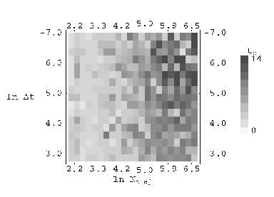
Figure 4.3: The stability time $t_{c}$ as a function of the time step $\Delta t$ and number $N_{\mathrm{traj}}$ of trajectories. We have used a window size $\Delta t_{W}=1.0$ here.

Chapter 5 Beables for Quantum Control

Beable methods offer two potential benefits in simulating quantum systems. We have already discussed how beables can help to define iterative numerical algorithms for simulating dynamics over an associated classical state space. But the beale framework also offers the possibility of a more concrete physical interpretation of simulation results themselves. Moreover, when we are interested not only in properties of some final state but also questions concering exactly how that final state was arrived at, beables can be of use. One current research area in particular is prone to such questions: quantum control of molecular systems via pulse-shaped lasers.

Advances in amplitude and phase modulation for ultrafast lasers, fast detection techniques, and their integration via closed-loop algorithms have made it possible to control the dynamics of a variety of quantum systems in the laboratory. Excitation may be either in the strong or weak field regime, with the goal of obtaining some desired final state. Success in achieving that goal is gauged by a detected signal (e.g., the mass spectrum in the case of selective molecular fragmentation), and this information is fed back into a learning algorithm [38], which alters the laser pulse shape for the next round of experiments. High duty cycles of $\sim 0.1$ seconds or less per control experiment make it possible to iterate this process many times and perform efficient experimental searches over a control parameter space defining the laser pulse shape.

As an example of this process, experiments have employed closed-loop methods for selective fragmentation and ionization of organic [39] and organometallic [40] [41] compounds, as well as for enhancing optical response in solid-state and other chemical systems [42] [43] [44] [45]. Yields of targeted species are typically enhanced considerably over those obtained by non-optimized methods. It is found that the optimal pulse shapes achieving these enhancements can be quite complicated, and understanding their physical significance has proven difficult. The same general observations also apply to the many optimal control design simulations carried out in recent years [46] [47] [48] [49].

This chapter will address the identification of control mechanisms in theoretical calculations as well as for direct application in the laboratory by offering a definition of mechanism in terms of beable trajectories.

5.1 Beables and Quantum Theory

Consider a control problem posed in terms of the quantum evolution

$$\mathrm{i}\hbar\frac{d}{dt}|\psi(t)\rangle=(H_{0}-\mu E(t))|\psi(t)\rangle$$ (5.1)

over a finite dimensional Hilbert space with basis $|n\rangle$ where $n=0,1,2,\ldots$. Here $H(t)=H_{0}-\mu E(t)$ incorporates the effect of the control field $E(t)$ via the dipole moment operator $\mu$, and we can explicitly follow the evolution of $|\psi\rangle$ into a desired final state $|\psi(t_{\mathrm{f}})\rangle$.

We are concerned with the question: what is the importance of a given sequence $n_{1}\rightarrow n_{2}\rightarrow\cdots$ of actual transitions—or, more specifically, of a given trajectory defined as a function $n(t)$ of time—in achieving the desired final state $|\psi(t_{\mathrm{f}})\rangle$? In other words, it is clear that the system is being driven into a desired state, but can we find a physical picture of how this is being accomplished?

A conventional answer to the question raised above, essentially that given by Bohr [54] on first seeing Feynman’s path integral, is to reject the question as ill-posed because quantum mechanics is said to forbid consideration of precisely defined trajectories over the classical state space $\{n\}$. Nevertheless, it is well established that there exist dynamical models generating an ensemble of trajectories $n(t)$ whose statistical properties exactly match those associated with $|\psi(t)\rangle$ at each $t$. In the case of a continuous state space, the first such model (as sketched in Chapter 4) was that of de Broglie [50], later rediscovered and completed by Bohm [30]. They reintroduce classical-like particle trajectories into quantum theory by taking the probability current $\mathbf{J}[\psi]$ to describe a statistical ensemble of real particles. So,

$$\mathbf{v}=\frac{\mathbf{J}}{|\psi|^{2}}=\mathrm{Re}\left\{-\mathrm{i}\frac{\hbar}{m}\frac{\nabla\psi(\mathbf{x},t)}{\psi(\mathbf{x},t)}\right\}$$ (5.2)

gives the velocity of a particle with mass $m$ and position $\mathbf{x}$ at time $t$, in de Broglie-Bohm (dBB) theory. The physical particle is taken to exist independently of, but also to have its motion determined by, the wavefunction $\psi$. The time evolution of $\psi$ itself is just given by the Schrodinger equation.

Bohm developed a full account of how ensembles of such classical-like particles could reproduce the predictions of quantum mechanics. A basic issue is to compare $\psi(\mathbf{x},t)$ with the statistical distribution $P(\mathbf{x},t)$ describing an ensemble of particles evolving by (5.2). One can show that if the initial distribution of particles satisfies $P(\mathbf{x},0)=|\psi(\mathbf{x},0)|^{2}$, then $P(\mathbf{x},t)=|\psi(\mathbf{x},t)|^{2}$ will hold for all $t>0$. That is, if the ensemble is initially in the “quantum equilibrium” distribution given by $|\psi(\mathbf{x},0)|^{2}$, the dynamics—(5.2) for the particles, and the Schrodinger equation for $\psi$—will preserve this equilibrium, consistent with the predictions of standard quantum theory [30][51]. The result is easily generalized to arbitrary interacting $N$-particle systems by taking $\mathbf{x}$ as a point in the $3N$ dimensional configuration space.

In dBB theory the position representation has a special status. While one may still regard $\psi$ as a basis-independent object, the particle dynamics is given by (5.2) specifically in terms of $\langle\mathbf{x}|\psi\rangle$ rather than $\langle\mathbf{p}|\psi\rangle$ or some other representation. But, it is easy to formulate analogs of dBB theory in different bases. For instance, one might choose the momentum values $\mathbf{p}$ as the beables of the theory, and the dBB trajectories $\mathbf{x}(t)$ would be replaced by momentum space trajectories $\mathbf{p}(t)$.

In the context of a finite dimensional Hilbert space with basis $|n\rangle$, the beables can be taken as the sites $n$ of the classical state space $\{n\}$ analogous to $\{\mathbf{x}\}$ or $\{\mathbf{p}\}$. Some law analogous to (5.2) must be given to generate beable trajectories $n(t)$ over the state space. Such trajectories would provide a physical picture of the quantum transitions induced by a control field $E(t)$. John Bell’s definition (4.16) of stochastic trajectories over $\{n\}$ is one such law. Moreover, it can be shown [55] to be minimal in the sense that any alternative law will require higher jump rates—in fact, these higher rates are such that the increased flux associated with jumping from $n$ to $m$ is found to exactly counterbalance that in the opposite direction.

The answer to the initial question regarding the importance of a given trajectory in achieving the desired state $|\psi(t_{\mathrm{f}})\rangle$ is quite simple in Bell’s theory. The importance may be taken as just the path probability (4.23).

The argument given in Chapter §4 for the equivalence of Bell’s theory and ordinary quantum mechanics ensures that the path probabilities $\mathrm{Prob}(\mathcal{P})$ are consistent with the quantum distribution $|\psi_{n}(t)|^{2}$ governing observables. But, it should be noted that Bell’s theory is not unique in this regard. The rule (4.16) may be altered in non-trivial ways while preserving the master equation (4.19) [55], although Bell’s rule is minimal in the sense mentioned above. The definition (4.16) might even be changed in ways that do not preserve (4.19), if one is willing to relinquish a strict probability interpretation for the trajectories [52].

In general, there are many different ways to assign probabilities to trajectories that all result in the same time-dependent occupation probabilities $P_{n}(t)$. The predictions of quantum mechanics, therefore, cannot select a single assignment. This non-uniqueness at the root of quantum mechanism identification can be dealt with only by reference to the simplicity and explanatory power of a given mechanism definition. Below we adopt the definition (4.16).

5.2 Simulating Beables in Quantum Control

Our ultimate goal is to obtain dynamical mechanism information directly from experimental data associated with the closed-loop control field optimization, without pre-existing knowledge of the system Hamiltonian or wavefunction. Methods employing Bell’s theory for this purpose are presented in §5.4, but first we shall study control mechanisms for a model system whose Hilbert space and quantum evolution are given explicitly in numerical simulations.

Consider a quantum-optical system with level energies $\hbar\omega_{n}$ and dipole moments $\mu_{nm}$. Applying an external laser field $E(t)$, the Hamiltonian in the interaction picture is

$$H_{I}=E(t)\sum_{n\,m}\mu_{nm}e^{\mathrm{i}\omega_{nm}t}|n\rangle\langle m|$$ (5.3)

where $\omega_{nm}\equiv\omega_{n}-\omega_{m}$. We will drop the subscript $I$ from now on. The definition here of $|n\rangle$ as interaction picture states has the affect of eliminating larger contributions to the jump probabilities $T_{nm}$ from the $\hbar\omega$ terms, hence reducing the overall frequency of jumps. $E(t)$ is assumed to be given by an independent optimization algorithm designed to, for example, maximally transfer population from $|n_{\mathrm{i}}\rangle$ to $|n_{\mathrm{f}}\rangle$.

A simple second-order Schrodinger propagator was used to solve (5.1) in the interaction picture, relying on a factorization of the evolution operator as

$$\mathcal{T}\left\{e^{-\frac{\mathrm{i}}{\hbar}\int_{0}^{t}H(s)ds}\right\}=\prod_{p=0}^{N-1}\mathcal{T}\left\{e^{-\frac{\mathrm{i}}{\hbar}\int_{t_{p}}^{t_{p+1}}H(s)ds}\right\}$$ (5.4)

where $t_{p}=p\epsilon\equiv pt_{\mathrm{f}}/N$ and $\mathcal{T}$ is the time-ordering symbol. Choosing a time step $\epsilon\ll\hbar/\mu E$, we can approximate (5.4) by dropping the $\mathcal{T}$ operations on the right hand side and computing the integrals directly. In doing this an error is accrued per time step given by the Baker-Hausdorf identity $e^{A+B}=e^{A}e^{B}e^{-\frac{1}{2}[A,B]+\cdots}$ as

$$\frac{1}{\hbar^{2}}\int_{t_{p}}^{t_{p+1}}\int_{t_{p}}^{t_{p+1}}[H(r),H(s)]\,dr\,ds\;\sim\;\left(\frac{\mu E}{\hbar}\right)^{2}\epsilon^{3}\omega\,.$$ (5.5)

The right hand estimate is obtained by expanding $H(r)$ to first order about $r=s$ and noticing that the $E^{\prime}(s)$ term in $H^{\prime}(s)$ commutes with $H(s)$. The error (5.5) would generally dominate third order terms like $(\mu E\epsilon/\hbar)^{3}$.

If the control field is given as $E(t)=\mathrm{Re}\{\sum_{i}\alpha_{i}E_{i}(t)\}$, where

$$E_{i}(t)=A(t)e^{\mathrm{i}(\phi(t)+\omega_{i}^{\mathrm{c}}t)}$$

with $A(t)$ and $\phi(t)$ possibly adiabatic, we can evaluate $\int H(s)ds$ by writing

$$\int_{t_{p}}^{t_{p+1}}\mu E_{i}(s)e^{\mathrm{i}\omega s}ds\;\approx\;\frac{\mu A(t_{p})e^{\mathrm{i}\phi(t_{p})}}{\mathrm{i}(\omega+\omega_{i}^{\mathrm{c}})}\left(e^{\mathrm{i}(\omega+\omega_{i}^{\mathrm{c}})t_{p+1}}-e^{\mathrm{i}(\omega+\omega_{i}^{\mathrm{c}})t_{p}}\right)\;.$$ (5.6)

(Simply writing $\int H(s)ds\approx\epsilon H(t_{p})$ is not appropriate because we do not want to exclude weak field excitation, i.e. $\mu E\ll\hbar\omega$, so that $\omega\epsilon\sim 1$ may hold.) Thus in the adiabatic case $|\psi(t)\rangle$ can be propagated in steps determined by $A(t)$ and $\phi(t)$ rather than the phase factors $e^{\mathrm{i}\omega t}$.

Consider the evolution of beable trajectories according to (4.16), which appears to require a time step small enough that each part of $H$, including the $e^{\mathrm{i}\omega t}$ terms, not vary much over the step. Nevertheless, the total probability of jumping from $m$ to $n$ over $(t_{p},t_{p+1})$ is given by the integral $\int T_{nm}(s)ds$ over that range with $\sim(\mu E\epsilon/\hbar)^{2}$ corrections. Thus we can take an effective jump probability for the interval $(t_{p},t_{p+1})$ as given by (4.16) with

$$z_{nm}(t_{p})\;\approx\;-\frac{\psi_{n}(t_{p})^{\ast}}{\psi_{m}(t_{p})^{\ast}}\frac{\mathrm{i}}{\hbar\epsilon}\int_{t_{p}}^{t_{p+1}}H_{nm}(s)ds$$ (5.7)

evaluated using (5.6). Note that we have included a factor of $1/\hbar$ explicitly into the definition (4.17) of $z_{nm}$. If $\omega\epsilon\ll 1$ does not hold, care must be taken to extend the integration in (5.7) only over $t\in(t_{p},t_{p+1})$ for which $\mathrm{Re}\{z_{nm}(t)\}>0$, leading to additional boundary terms in the phase difference part of (5.6). Moving the $\psi^{\ast}$ ratio outside the integral in (5.7) produces an error per time step of order

$$\frac{\epsilon^{2}H}{\hbar}\frac{\partial\psi}{\partial t}\;\sim\;\left(\frac{\mu E\epsilon}{\hbar}\right)^{2}$$

which is again comparable to (5.5). Therefore beable trajectories may be propagated in steps determined by the possibly adiabatic amplitude $A(t)$ and phase $\phi(t)$, i.e. synchronously with the Schrodinger propagator.

5.3 Mechanism Analysis for a Model 7-Level System

The beable trajectory methodology for identification of control mechanisms will be illustrated with a 7-level system where $\omega_{n}$ and $\mu_{nm}$ are given in Fig. 5.1. The (non-adiabatic) control field $E(t)$ shown in Fig. 5.2 is obtained from a steepest descents algorithm over the space of field histories [53]. It is optimized to transfer population from the ground state $|0\rangle$ to the highest excited state $|6\rangle$. By $t=100$ fs, the transfer is found to be completed with approximately 97% efficiency (see Fig. 5.3).

Figure 5.1: The model 7-level system $|n\rangle$ with $n=0,1,\ldots,6$. The transition frequencies $\omega_{nm}$ in units of fs^-1 are shown on the right, and non-zero dipole matrix elements $\mu_{nm}$ in units of $10^{-30}$ C$\cdot$m are indicated by dotted lines.

Together with the second-order Schrodinger propagator, using time step $\epsilon=.025$ fs, an ensemble of $N_{\mathrm{traj}}=10^{5}$ beable trajectories is evolved, all starting in the ground state $n=0$ at $t=0$. At each time step, a given beable at site $m$ is randomly made either to jump to a neighboring site $n\neq m$ according to the probabilities $T_{nm}\epsilon$ given by (4.16) with (5.7), or else stay at $m$. Four sample trajectories are shown in Fig. 5.4. As a check, one can count the number of beables residing on each site $n$ at time $t$ to estimate the occupation probabilities $P_{n}(t)$ and verify that they match the quantum prescriptions $|\psi_{n}(t)|^{2}$. The finite-ensemble deviations are observed to be consistent with a $(N_{\mathrm{traj}})^{-1/2}$ convergence law.

Figure 5.2: Electric field $E(t)$ in $V/\mathrm{\AA}$ obtained from an optimization algorithm for population transfer from $|0\rangle$ to $|6\rangle$ [53].

About 60% of the trajectories generated are found to involve four jumps, and of these the trajectories passing through sites $n=2,5$ are noticeably more probable than those passing through $n=1,4$. 6-jump trajectories comprise about 30% of the ensemble. And it becomes increasingly less likely to find trajectories with more and more jumps. The largest number of jumps observed in a single trajectory was 14. Three such trajectories occurred out of the ensemble total $10^{5}$.

A natural expectation is that the optimal field $E(t)$ would concentrate on the higher probability trajectories and not waste much effort on guiding highly improbable trajectories, such as the 14-jumpers, to the target state $n=6$, as the latter have essentially no impact on the control objective (final population of the target state). Interestingly, though, the vast majority of even the lowest probability trajectories are still guided to $n=6$. Apparently, the optimal field is able to coordinate its effect on low probability trajectories with that on other trajectories at no real detriment to the latter. We shall come back to this point later.

Figure 5.3: Population $|\psi_{6}(t)|^{2}$ as a function of time (fs). Detail for small $t$ is shown in the inset (same units).

One way to conveniently categorize the large set of trajectories, each expressible as a sequence of time-labeled jumps $(t_{1},n_{1})\rightarrow(t_{2},n_{2})\rightarrow\cdots$, is to drop the time labels, leaving only the “pathway” $n_{1}\rightarrow n_{2}\rightarrow\cdots$. The importance of a given pathway is then computed as the frequency of trajectories associated with that pathway. Table 5.1 lists some important and/or interesting pathways and their probabilities.

probability	pathway
0.19	0 2 3 5 6
0.16	0 2 3 4 6
0.14	0 1 3 5 6
0.12	0 1 3 4 6
0.018	0 2 3 5 6 5 6
0.005	0 2
0.0007	0 2 3 5 6 4 3 5 6

Table 5.1: The five most probable pathways, followed by the highest probability pathway failing to reach $n=6$ at $t=100$ fs, and then the highest probability pathway involving a topologically non-trivial cycle in state space. The fractional error in the pathway probability $P$ is given roughly by $(10^{5}P)^{-1/2}$.

Fig. 5.5 shows some typical trajectories associated with the first and fifth pathways listed in Table 5.1—involving 4 and 6 jumps respectively. $E(t)$ guides the 4-jumpers upward in energy, and they begin to arrive at $n=6$ around $t=80$ fs, early enough that stragglers can catch up but too late for the over-achievers of the group to head off elsewhere. This corresponds to the onset of heavy growth for $|\psi_{6}(t)|^{2}$ around $t=80$ fs (see Fig. 5.3). The 6-jumpers first reach $n=6$ around $t=50$ fs, but almost all fall back to $n=5$ by $t=80$ fs, reuniting with the 4-jumpers just as they begin to jump up to $n=6$. These 6-jumpers, along with other high-order contributions, thus explain the small surge in $|\psi_{6}(t)|^{2}$ between 50 and 80 fs. Another much smaller surge around $t=30$ fs and one still smaller around $t=20$ fs (see inset of Fig. 5.3) are attributable to 8-th and higher order trajectories “ringing” back and forth on $5\leftrightarrow 6$.

Figure 5.4: One each of the 4, 6, 8, and 10-jump trajectories generated by the jump rule (4.16) are shown with their sites $n$ plotted against time. For viewing purposes, we have displaced them a small amount vertically from each other and tilted the jump lines slightly away from the vertical.

For $t\in(70\mbox{ fs},80\mbox{ fs})$, many of the 6-jumpers are at $n=6$ and need to be de-excited on the $6\rightarrow 5$ transition before they can jump back up to $n=6$. Simultaneously, many of the 4-jumpers are at $n=5$ and should not be prematurely excited on $5\rightarrow 6$, lest they not remain at $n=6$ through $t=100$ fs. The optimal field thus faces a conundrum: how to stimulate the $2\leftrightarrow 6$ transition preferentially for the 6-jumpers (in $n=6$) over the 4-jumpers (in $n=5$). The means by which this feat is accomplished may be understood by reference to the jump rule (4.16). $E(t)$ induces jumps through the explicit $H_{nm}(t)$ factor but also through the $\psi^{\ast}$ quotient, which depends on $E(t)$ through $(\ref{schrod})$. In particular, (4.18) implies that at any one time $t$ jumps on this transition must be either all upward or all downward. The active direction is switched back and forth according to the sign of $\mathrm{Re}\{z_{65}(t)\}$.

Figure 5.5: A sample of 20 trajectories each from the pathways 0 2 3 5 6 and 0 2 3 5 6 5 6.

Fig. 5.6 plots $|E(t)|$ and $\mathrm{Re}\{z_{65}(t)\}$, which controls the upward jump rate $T_{65}(t)$. For $t\in(70\mbox{ fs},80\mbox{ fs})$ one sees that when $|E(t)|$ is large, most often $\mathrm{Re}\{z_{65}(t)\}$ dips below zero, disallowing any upward jumps. The correlation coefficient between $|E(t)|$ and $\mathrm{Re}\{z_{65}(t)\}$ in this range is $-0.4955$. On the other hand, the correlation between $|E(t)|$ and $\mathrm{Re}\{z_{56}(t)\}$, which controls downward jumping, is $+0.4475$ over the same range.

Figure 5.6: The optimal field modulus $|E(t)|$ (dotted line) and $\mathrm{Re}\{z_{65}(t)\}$ (full line) in $\mbox{fs}^{-1}$ over the range $(70\mbox{ fs},80\mbox{ fs})$. Their anticorrelation causes beables to be preferentially selected for the downward transition $6\rightarrow 5$ over the upward transition $5\rightarrow 6$.

Looking at the trajectories in more detail, one notices a distinct bunching of jumps. Beables tend to jump together in narrow time bands, or else to abstain in unison from jumping. This behavior can be gauged by calculating the two-time jump-jump correlation function:

$$J_{\Omega}^{(2)}(\tau)\equiv\frac{1}{N}\sum_{p=0}^{N-1}J_{\Omega}(t_{p})J_{\Omega}(t_{p}+\tau)$$

where $J_{\Omega}(t)$ is the number of jumps of type $\Omega$ occurring in $(t,t+\epsilon)$, and $\Omega$ is a subset of the entire ensemble of trajectories. For instance, the two-time function with $\Omega$ taken as the set of jumps on the $5\rightarrow 6$ transition is plotted in Fig. 5.7. The fs time-scale oscillations correspond to the level splittings $\omega_{nm}$ and the dominant frequency components of $E(t)$. Enhanced correlations around $\tau=0$ correspond to the jump bunching noticeable in the trajectories. Two side-bands around $\tau=\pm 40$ fs are associated with 6-jump and higher order trajectories that go up, down, and up again on $5\leftrightarrow 6$ over the approximate time window $(50\mbox{ fs},90\mbox{ fs})$. This conclusion can be verified by computing two-time functions with $\Omega$ specialized to particular pathways. Other much smaller features for $|\tau|>60$ fs (see inset of Fig. 5.7) are attributable to higher order trajectories ringing on $5\leftrightarrow 6$.

Figure 5.7: Jump correlation function $J_{\Omega}^{(2)}(\tau)$ associated with jumps on $5\rightarrow 6$, plotted against the delay time $\tau$ (fs) for the ensemble of $10^{5}$ trajectories. Detail for large $\tau$ is shown in the inset (same units).

In general, the fs oscillations characteristic of these two-time functions show that $E(t)$ works in an essentially discrete way, turning on the flow of beables over a given transition and then turning it off with a duty cycle of $\approx 2$ fs. The associated bandwidth of $\approx 0.5\mbox{ fs}^{-1}$ is small enough to discriminate between all non-degenerate $\omega_{nm}$ except between $\omega_{35}(=\omega_{34})$ and $\omega_{56}(=\omega_{46})$, which differ by only $0.12\mbox{ fs}^{-1}$. This circumstance leaves effectively three distinguishable transitions. With a total time of 100 fs, the control field $E(t)$ can potentially enact roughly $150$ separate flow operations. The fact that trajectories with pathway probability $\ll 1$% are still almost always guided successfully to $n=6$ suggests that these $\sim 150$ operations are more than necessary to obtain the 97% success rate achieved by the optimal control algorithm in this simulation. It appears that the algorithm actively sweeps these aberrant trajectories back into the mainstream so as to maximize even their minute contribution to the control objective.

5.4 Control Mechanism Identification in The Laboratory

Using these beable trajectory methods to extract mechanism information directly from closed-loop data is complicated by the fact that we cannot assume knowledge of a time-dependent wavefunction, Hamiltonian, or possibly even the energy level structure of the system. Frequently in the laboratory, the only available information consists of final state population measurements and knowledge of the control field $E(t)$.

The following analysis aims to show how a limited statistical characterization of beable trajectories may be generated from laboratory data associated with a given optimal control field. In particular, we will show how to extract $j_{\mathrm{min}}$, the minimum number of jumps necessary to reach the final state $n_{\mathrm{f}}$ from the initial state $n_{\mathrm{i}}$; also $\langle j_{\mathcal{P}}\rangle$, the average number of such jumps over an ensemble of beable trajectories; and possibly higher moments $\langle(j_{\mathcal{P}})^{k}\rangle$ as well. After a general formulation of this analysis is presented, it will be applied to simulated experimental data in the case of the model 7-level system considered above.

We propose to obtain mechanism information by examining the effect on the final state population $|\psi_{n_{\mathrm{f}}}(t_{\mathrm{f}})|^{2}$ of variations in the control field away from optimality. Detecting only this one population, i.e. the control objective itself, limits how much mechanism information we can gain. It may be possible to obtain a more detailed understanding of a given mechanism by probing additional aspects of the system at times other than just $t_{\mathrm{f}}$, and this may be done either in our present framework or through extensive spectroscopic methods. One expects there will always be a trade-off between the complexity of such methods and the level of mechanistic detail they reveal.

Consider a particularly simple scheme wherein the amplitude of the control field is modulated by a constant $\mathcal{M}$ independent of time:

$$E(t)\rightarrow\tilde{E}(t)=\mathcal{M}E(t)$$

giving rise to a new time-dependent solution $|\tilde{\psi}(t)\rangle$—in particular, a new final state population $|\tilde{\psi}_{n_{\mathrm{f}}}(t_{\mathrm{f}})|^{2}$ and new path probabilities P$\widetilde{\mathrm{rob}}(\mathcal{P})$. These quantities are obtained by taking $T_{nm}\rightarrow\tilde{T}_{nm}$ in (4.23), which is to say using $\tilde{E}(t)$ and $\tilde{\psi}_{n}(t)$ in the jump rule (4.16).

To express P$\widetilde{\mathrm{rob}}(\mathcal{P})$ in terms of Prob$(\mathcal{P})$, we can write

$$\prod_{p\in J}\tilde{T}_{n_{p+1}n_{p}} = \mathcal{M}^{j_{\mathcal{P}}}\prod_{p\in J}T_{n_{p+1}n_{p}}\prod_{p\in J}\frac{\cos\tilde{\phi}_{p}}{\cos\phi_{p}}\;\times$$ (5.8)

$$\;\;\prod_{p\in J}\frac{|\tilde{\psi}_{n_{p+1}}(t_{p})|}{|\tilde{\psi}_{n_{p}}(t_{p})|}\left(\prod_{p\in J}\frac{|\psi_{n_{p+1}}(t_{p})|}{|\psi_{n_{p}}(t_{p})|}\right)^{-1}$$

where $j_{\mathcal{P}}$ is the number of jumps in $\mathcal{P}$ and

$$\tilde{\phi}_{p}\;\equiv\;\arg\left(-\mathrm{i}H_{n_{p+1}n_{p}}\frac{\tilde{\psi}_{n_{p+1}}(t_{p})}{\tilde{\psi}_{n_{p}}(t_{p})}\right)\,.$$

To simplify (5.8), note that if $j_{\mathcal{P}}$ were very large, then successive terms in each of the last two products would tend to cancel, leaving only endpoint contributions. Making the reasonable approximation that they do completely cancel yields

$$\prod_{p\in J}\tilde{T}_{n_{p+1}n_{p}}\;\approx\;\mathcal{M}^{j_{\mathcal{P}}}\,\frac{|\tilde{\psi}_{n_{\mathrm{f}}}(t_{\mathrm{f}})|}{|\psi_{n_{\mathrm{f}}}(t_{\mathrm{f}})|}\,\prod_{p\in J}T_{n_{p+1}n_{p}}\prod_{p\in J}\frac{\cos\tilde{\phi}_{p}}{\cos\phi_{p}}\,.$$ (5.9)

Further, we can make the expansion

$$-\ln\prod_{p\in J}\frac{\cos\tilde{\phi}_{p}}{\cos\phi_{p}}\;=\;a_{\mathcal{P}}^{(1)}(\mathcal{M}-1)+a_{\mathcal{P}}^{(2)}(\mathcal{M}-1)^{2}+\cdots$$

about $\mathcal{M}=1$, where the $a_{\mathcal{P}}^{(i)}$ depend on the path $\mathcal{P}$ but not on $\mathcal{M}$. And similarly:

$$-\ln\prod_{p\notin J}\left(1-\epsilon{\textstyle\sum_{n}^{\prime}}\tilde{T}_{nn_{p}}\right) \approx \epsilon{\textstyle\sum_{p\notin J}}{\textstyle\sum_{n}^{\prime}}\tilde{T}_{nn_{p}}$$

$$= \epsilon{\textstyle\sum_{p\notin J}}{\textstyle\sum_{n}^{\prime}}T_{nn_{p}}+b_{\mathcal{P}}^{(1)}(\mathcal{M}-1)+\cdots$$

Combining these expansions gives a relationship between the path probabilities P$\widetilde{\mathrm{rob}}(\mathcal{P})$ in the modulated case and those, Prob$(\mathcal{P})$, in the unmodulated case, which are the ones containing mechanism information regarding the actual optimal control field $E(t)$. We can thus write the final population as

$$|\tilde{\psi}_{n_{\mathrm{f}}}(t_{\mathrm{f}})|^{2} = \sum_{\mathcal{P}}|\psi_{n_{0}}(0)|^{2}\,\mbox{P$\widetilde{\mathrm{rob}}(\mathcal{P})$}$$

$$\approx \frac{|\tilde{\psi}_{n_{\mathrm{f}}}(t_{\mathrm{f}})|}{|\psi_{n_{\mathrm{f}}}(t_{\mathrm{f}})|}\sum_{\mathcal{P}}|\psi_{n_{0}}(0)|^{2}\mathcal{M}^{j_{\mathcal{P}}}e^{-a_{\mathcal{P}}(\mathcal{M}-1)}\,\mathrm{Prob}(\mathcal{P})$$

where $a_{\mathcal{P}}\equiv a_{\mathcal{P}}^{(1)}+b_{\mathcal{P}}^{(1)}$, and higher order terms in the expansion have been dropped. (This approximation is not as crude as it might seem, since for small $\mathcal{M}$ away from 1, the behavior of $|\tilde{\psi}_{n_{\mathrm{f}}}(t_{\mathrm{f}})|^{2}$ is dominated by the $\mathcal{M}^{j_{\mathcal{P}}}$ factor.) Cancelling one power of $|\tilde{\psi}_{n_{\mathrm{f}}}(t_{\mathrm{f}})|$, and recalling that the sum is taken only over paths ending on $n=n_{\mathrm{f}}$ so that $|\psi_{n_{\mathrm{f}}}(t_{\mathrm{f}})|^{2}=\sum_{\mathcal{P}}\mathrm{Prob}(\mathcal{P})$, we have

$$|\tilde{\psi}_{n_{\mathrm{f}}}(t_{\mathrm{f}})|\;\approx\;|\psi_{n_{\mathrm{f}}}(t_{\mathrm{f}})|\left\langle\mathcal{M}^{j_{\mathcal{P}}}e^{-a_{\mathcal{P}}(\mathcal{M}-1)}\right\rangle$$ (5.10)

where $\langle\cdots\rangle$ denotes an average over the trajectory ensemble generated by the (unmodulated) optimal field $E(t)$. Beables in this ensemble are taken as initially distributed at $t=0$ according to $|\psi_{n}(0)|^{2}$, and only trajectories that successfully reach $n=n_{\mathrm{f}}$ at $t=t_{\mathrm{f}}$ are counted.

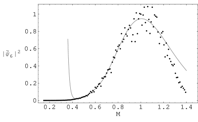
Figure 5.8: The best fit of (5.12) to the simulated $|\tilde{\psi}_{n_{\mathrm{f}}}(t_{\mathrm{f}})|^{2}$ data (10% noise) as a function of $\mathcal{M}$; it occurs over the fitting range $\mathcal{M}\in(.44,.92)$.

Note that for $\mathcal{M}$ close enough to 0, the minimum value $j_{\mathrm{min}}$ taken on by $j_{\mathcal{P}}$ will dominate the expectation value in (5.10), and

$$\ln|\tilde{\psi}_{n_{\mathrm{f}}}(t_{\mathrm{f}})|=j_{\mathrm{min}}\ln\mathcal{M}+\mathrm{O}(1)$$ (5.11)

gives the dominant behavior independent of $a_{\mathcal{P}}$. If we suppose that $a_{\mathcal{P}}$, where it is relevant, depends primarily on the endpoints of $\mathcal{P}$, which are fixed, and only weakly on the rest of the path, then $a_{\mathcal{P}}$ can be approximated by some characteristic value $a$. Putting $\mathcal{M}^{j_{\mathcal{P}}}=e^{j_{\mathcal{P}}\ln\mathcal{M}}$ in (5.10) and expanding in powers of $\ln\mathcal{M}$ now gives

$$|\tilde{\psi}_{n_{\mathrm{f}}}(t_{\mathrm{f}})|\;\approx\;|\psi_{n_{\mathrm{f}}}(t_{\mathrm{f}})|\,e^{-a(\mathcal{M}-1)}\sum_{k=0}^{\infty}\frac{\langle(j_{\mathcal{P}})^{k}\rangle}{k!}(\ln\mathcal{M})^{k}$$ (5.12)

for the final state population under a modulated field, expressed in terms of the desired statistical properties of the trajectory ensemble under the optimal field itself. Here, $a$ enters as an additional parameter that must be extracted from the data. Equations (5.11) and (5.12) form the working relations to extract mechanism information from laboratory data.

5.5 Simulated Experiments on a 7-Level System

In order to extract quantities like $\langle j_{\mathcal{P}}\rangle$ using the results (5.11) and (5.12) data must be generated for the final state population $|\tilde{\psi}_{n_{\mathrm{f}}}(t_{\mathrm{f}})|^{2}$ at many values of the modulation factor $\mathcal{M}$ over some range $(\mathcal{M}_{\mathrm{min}},\mathcal{M}_{\mathrm{max}})\sim(0,1.5)$. The desired quantities are obtained as parameters in fitting (5.11) and (5.12) to the data as a function of $\mathcal{M}$.

One set of simulated data for the above 7-level system is shown in Fig. 5.8; the sampling increment is $\Delta M=.01$. Noise has been introduced by multiplying the exact $|\tilde{\psi}_{n_{\mathrm{f}}}(t_{\mathrm{f}})|^{2}$ values by an independent Gaussian-distributed random number for each value of $\mathcal{M}$, where the distribution is chosen to have mean 1, and various standard deviations $\sigma$ have been sampled.

We can determine $j_{\mathrm{min}}$ from the data using (5.11), which implies

$$j_{\mathrm{min}}=\lim_{\mathcal{M}\rightarrow 0}\frac{d\ln|\tilde{\psi}_{n_{\mathrm{f}}}(t_{\mathrm{f}})|}{d\ln\mathcal{M}}\,.$$ (5.13)

For instance, Fig. 5.9 plots the derivative in (5.13), calculated with finite differences from the $|\tilde{\psi}_{n_{\mathrm{f}}}(t_{\mathrm{f}})|^{2}$ simulated data for $\sigma=.1$, which correctly gives $j_{\mathrm{min}}=4$ as the limiting value. Determination of $j_{\mathrm{min}}$ proved robust to multiplicative Gaussian noise up to the 40% level ($\sigma=.4$).

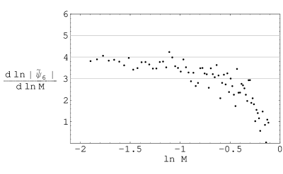
Figure 5.9: The derivative is calculated from simulated data with noise level $\sigma=.1$; its limiting value as $\ln\mathcal{M}\rightarrow-\infty$ gives $j_{\mathrm{min}}$.

The quantity $\langle j_{\mathcal{P}}\rangle$ is more difficult to extract, because while the sum in (5.12) converges to 0 as $\mathcal{M}\rightarrow 0$, the terms of the sum individually diverge and must cancel in a delicate manner. Therefore truncating the sum to an upper limit $k_{\mathrm{max}}$ becomes a very bad approximation near $\mathcal{M}=0$. This unstable behavior can be controlled by carefully setting the range $(\mathcal{M}_{\mathrm{min}},\mathcal{M}_{\mathrm{max}})$ of data to be fitted, given a choice of $k_{\mathrm{max}}$.

It is also convenient to constrain the fit by the previous determination of $j_{\mathrm{min}}=4$. We have done this by noting that if $E(t)$ is truly optimal, then $|\tilde{\psi}_{n_{\mathrm{f}}}(t_{\mathrm{f}})|$ must have a maximum at $\mathcal{M}=1$, which implies that $a=\langle j_{\mathcal{P}}\rangle$. This can be used as a weaker constraint on the auxiliary parameter $a$ by just requiring $a>j_{\mathrm{min}}=4$ in the fit without necessarily supposing that $E(t)$ is exactly optimal. We then check that $a\approx\langle j_{\mathcal{P}}\rangle$ is satisfied in the fit. Fig. 5.8 shows one such fit where the fitting range is $\mathcal{M}\in(.44,.92)$. One can see that the fit closely tracks the data for $\mathcal{M}$ in this range but quickly diverges from the data just below $\mathcal{M}=.44$ (and, less severely, above $\mathcal{M}=.92$) due to the sum-truncation instability mentioned previously.

In order to identify appropriate ranges in general, we have searched over all combinations such that

$$\begin{array}[]{c}\begin{array}[]{lcccr}.2&<&\mathcal{M}_{\mathrm{min}}&<&.8\\ .7&<&\mathcal{M}_{\mathrm{max}}&<&1.6\\ \end{array}\\ \mathcal{M}_{\mathrm{max}}-\mathcal{M}_{\mathrm{min}}>10\end{array}$$ (5.14)

Mathematica’s implementation of the Levenberg-Marquardt non-linear fitting algorithm was used on simulated data for each value of $\sigma$ between 0 and .5 with a .01 increment. The best fit at each $\sigma$ was used to determine the value of $\langle j_{\mathcal{P}}\rangle$ most consistent with the simulated data at the given noise level.

For this analysis $k_{\mathrm{max}}=4$ was chosen somewhat arbitrarily to balance computational cost and precision. In practice it is likely that the moments $\langle(j_{\mathcal{P}})^{k}\rangle$ for lower $k$ values will be most reliably extracted from the data, especially considering the laboratory noise. In the simulations it was found that $\langle j_{\mathcal{P}}\rangle$ could be reliably extracted, but higher moments were unstable and unreliable. For example, $\langle(j_{\mathcal{P}})^{2}\rangle$ was frequently found to lie slightly below the corresponding fit values for $\langle j_{\mathcal{P}}\rangle^{2}$, which is inconsistent with the interpretation of these values as statistical moments of an underlying random variable $j_{\mathcal{P}}$. Further constraints could be introduced to attempt to stabilize the extraction of higher moments, but care is needed so as not to overfit the data.

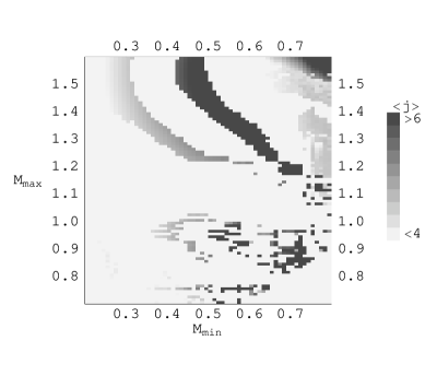
Figure 5.10: Fit values for $\langle j_{\mathcal{P}}\rangle$ over a set of different fitting ranges $(\mathcal{M}_{\mathrm{min}},\mathcal{M}_{\mathrm{min}})$; $\sigma=.1$ here.

Fig. 5.10 shows the $\langle j_{\mathcal{P}}\rangle$ values obtained by fitting data with $\sigma=.1$ for each choice of $(\mathcal{M}_{\mathrm{min}},\mathcal{M}_{\mathrm{max}})$ and Fig. 5.11 shows the corresponding quality of each fit as measured by its mean squared deviations. In Fig. 5.10, as well as in the corresponding plots for all other values of $\sigma$ studied, two diagonal strips emerge running above a set of smaller islands. The surrounding white “sea” comprises fits that give $\langle j_{\mathcal{P}}\rangle<4$, which we know to be ruled out by the determination of $j_{\mathrm{min}}$.

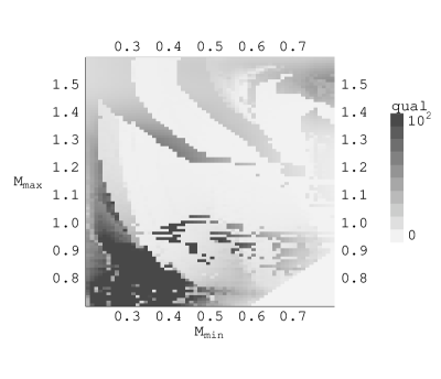
Figure 5.11: Fit qualities as measured by the inverse of the mean squared deviations between the simulated data and the fit; $\sigma=.1$ here. The highest fit quality appears at $(.44,.92)$.

A virtually identical pattern arises in the fit quality plots. The two strips and underlying islands are seen to give much better fits than the white sea. An additional connected region of good fits is found to extend across the lower-left corner of Fig. 5.11, nearly all of which are ruled out by $j_{\mathrm{min}}=4$. This connected region is somewhat pathological because much of it corresponds to fitting ranges that fail to capture the important behavior of $|\tilde{\psi}_{n_{\mathrm{f}}}(t_{\mathrm{f}})|^{2}$ near $\mathcal{M}=1$, and therefore can be ignored. Then the best fits for all values of $\sigma$ sampled are found to come from the cluster of islands at $\mathcal{M}_{\mathrm{max}}\approx.95$. As $\sigma$ is increased from 0 to .5, these islands flow from $\mathcal{M}_{\mathrm{min}}\approx.5$ to $\mathcal{M}_{\mathrm{min}}\approx.3$, carrying with them the best fit site. Note that the small triangular area in the lower right corner, most noticeable in Fig. 5.11, is a region excluded from consideration by the third constraint in (5.14).

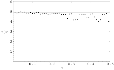
Figure 5.12: Best fit values for $\langle j_{\mathcal{P}}\rangle$ as a function of the noise level $\sigma$, compared to the exact value $\langle j_{\mathcal{P}}\rangle=4.907$ (gray line).

The best fit values of $\langle j_{\mathcal{P}}\rangle$ are shown as a function of $\sigma$ in Fig. 5.12. These values are to be compared with the exact result $\langle j_{\mathcal{P}}\rangle=4.907$ obtained from the trajectory ensemble calculations in §5.3, which require explicit knowledge of the level structure and dipole moments $\mu_{nm}$ of the system. The ramping behavior in Fig. 5.12 results from the sampling increment $\Delta\mathcal{M}$ of the simulated data. Transitioning between one ramp and another corresponds to the shifting of the best fit location by one or two units of $\Delta\mathcal{M}$.

These $\langle j_{\mathcal{P}}\rangle$ values are in good agreement (3% discrepancy) with the exact value for noise at the level of 0–25%. It should be noted that a qualitative change occurs in the case of no noise ($\sigma=0$), where the islands all disappear and the strips become extended much further on the downward diagonal. Inspecting the fits individually indicates that mean squared deviation does not give an adequate measure of fit quality in this special case. This anomaly seems due to the fact that, in the absence of Gaussian noise from experimental statistics, systematic deviations from (5.12) associated with the approximation (5.9) become important.

Since Bell’s model can be defined for any choice of basis $|n\rangle$, there is a more general question of how the above kind of mechanism analysis might vary with the choice of basis. Beyond that, Bell’s jump rule (4.16) itself permits generalization [55], providing additional freedom over which trajectory probability assignments may vary. The import of this freedom for mechanism identification remains to be determined.

Bibliography

- [1] R. Laughlin and D. Pines, PNAS 97 28-31 (2000).
- [2] R. Feynman, “Simulating physics with computers,” Int. J. Theor. Phys. 21 467 (1982).
- [3] S. Lloyd, “Universal Quantum Simulators,” Science 273 1073 (1996).
- [4] P. Shor, “Polynomial-Time Algorithms for Prime Factorization and Discrete Logarithms on a Quantum Computer,” SIAM J. Sci. Statist. Comput. 26 1484 (1997).
- [5] A. Peirce, M. Dahleh, and H. Rabitz, “Optimal Control of Quantum Mechanical Systems: Existence, Numerical Approximations, and Applications,” Phys. Rev. A 37 4950 (1988).
- [6] see Chapter 6 of John Preskill’s quantum computation notes on the web at http://www.theory.caltech.edu/people/preskill/ph229/index.html.
- [7] “Quantum computation with quantum dots and terahertz cavity quantum electrodynamics,” Phys. Rev. A 60 3508 (1999), quant-ph/9904096.
- [8] R. Landauer, “Is quantum mechanics useful?” Phil. Tran. R. Soc. Lond. 353 367 (1995).
- [9] P. Shor, “Scheme for reducing decoherence in quantum computer memory,” Phys. Rev. A 52 R2493 (1995).
- [10] M. H. Freedman and D. A. Meyer, “Projective plane and planar quantum codes,” quant-ph/9810055 (1998).
- [11] P. Shor, “Fault-tolerant quantum computation,” Proc. 37th Ann. Symp. on the Foundations of Computer Science, (IEEE Computer Society Press, Los Alamitos, CA, 1996), quant-ph/9605011.
- [12] J. Preskill, “Reliable Quantum Computers,” Proc. Roy. Soc. Lond. A 454 385 (1998).
- [13] E. Knill and R. Laflamme, “Concatenated quantum codes,” quant-ph/9608012.
- [14] E. Knill, R. Laflamme, and W. Zurek, “Threshold accuracy for quantum computation,” quant-ph/9610011; E. Knill, R. La amme, and W. H. Zurek, “Resilient quantum computation,” Science 279 342 (1998).
- [15] D. Aharonov and M. Ben-Or, “Fault-tolerant quantum computation with constant error,” Proc. 29th Ann. ACM Symp. on Theory of Computing, (ACM, New York, 1998), quant-ph/9611025.
- [16] C. Zalka, “Threshold estimate for fault-tolerant quantum computing,” quant-ph/9612028.
- [17] D. Gottesman, “Stabilizer codes and quantum error correction,” quant-ph/9705052 (1997); “Theory of fault-tolerant quantum computation,” Phys. Rev. A 57 127 (1998), quant-ph/9702029.
- [18] J. Preskill, “Fault-tolerant quantum computation,” in Introduction to Quantum Computation and Information, Hoi-Kwong Lo, Sandu Popescu, and Tim Spiller, (World Scientifc, New Jersey, 1998), quant-ph/9712048.
- [19] A. Kitaev, “Fault-tolerant quantum computation by anyons,” quant-ph/9707021 (1997).
- [20] S. Bravyi and A. Kitaev, “Quantum codes on a lattice with boundary,” quant-ph/9811052 (1998).
- [21] M. Freedman and D. Meyer, “Projective plane and planar quantum codes,” quant-ph/9810055 (1998).
- [22] E. Dennis, A. Kitaev, A. Landahl, J. Preskill, “Topological quantum memory,” J. Math. Phys. 43 4452-4505 (2002), quant-ph/0110143.
- [23] H. Barnum et al., Phys. Rev. A 57 4153 (1998).
- [24] D. Ceperley, M. Kalos, in Monte Carlo Methods in Statistical Mechanics, edited by K. Binder, Springer Verlag (1979).
- [25] H. Carmichael, Statistical Methods in Quantum Optics 1, Springer Verlag (1999).
- [26] J. Negele, H. Orland, Quantum Many-Particle Systems, Perseus (1998).
- [27] G. Parisi, Y. Wu., Sci. Sin. 24 483 (1981).
- [28] M. Davidson, Lett. Math. Phys. 3 271 (1979), quant-ph/0112063.
- [29] E. Nelson, Phys. Rev. 150 1079 (1966); Dynamical Theories of Brownian Motion, Princeton University Press (1967).
- [30] D. Bohm, Phys. Rev. 85 166 (1952); Phys. Rev. 85 180 (1952).
- [31] J. Moskowitz et al., J. Chem. Phys. 77 349 (1982).
- [32] S. Duane and J. Kogut, Phys. Rev. Lett. 55 2774 (1985).
- [33] S. Goldstein, private communication.
- [34] C. Lopreore and R. Wyatt, Phys. Rev. Lett. 85 895 (2000).
- [35] B. Dey, A. Askar, and H. Rabitz, J. Chem. Phys. 109 8770 (1998); X.-G. Hu, T.-S. Ho, H. Rabitz, Phys. Rev. E 61 5967 (2000).
- [36] J. Bell, “Beables for quantum field theory,” Speakable and unspeakable in quantum mechanics, Cambridge University Press (1987).
- [37] R. Feynman, Statistical Mechanics: A Set of Lectures, Addison-Wesley (1972), cf. 202.
- [38] R. Judson, H. Rabitz, Phys. Rev. Lett. 68 1500 (1992).
- [39] R. Levis, G. Menkir, H. Rabitz, Science 292 709 (2001).
- [40] A. Assion, T. Baumer, M. Bergt, T. Brixner, B. Kiefer, V. Seyfried, M. Strehle, G. Gerber, Science, 282 919 (1998).
- [41] S. Vajda, A. Bartelt, E. Kaposta, T. Leisner, C. Lupulescu, S. Minemoto, P. Francisco, L. Woste, Chem. Phys. 267 231 (2001).
- [42] J. Kunde, B. Baumann, S. Arlt, F. Morier-Genoud, U. Siegner, U. Keller, Appl. Phys. Lett. 77 924 (2000).
- [43] R. Bartels et al., Nature 406 164 (2000).
- [44] C. Bardeen et al., Chem. Phys. Lett. 280 151 (1997).
- [45] T. Weinacht, J. White, P. Bucksbaum, J. Phys. Chem. A 103 10166 (1999).
- [46] M. Dahleh, A. Peirce, H. Rabitz, Phys. Rev. A 37 4950 (1988).
- [47] R. Kosloff, S. Rice, P. Gaspard, S. Tersigni, D. Tannor, Chem. Phys. 139 201 (1989).
- [48] H. Rabitz, W. Zhu, Accts. Chem. Res. 33 572 (2000).
- [49] S. Rice, M. Zhao, Optical Control of Molecular Dynamics, Wiley (2000).
- [50] L. de Broglie, in Rapport au V’ieme Congres de Physique Solvay, Gauthier-Villars, Paris (1930).
- [51] D. Durr, S. Goldstein, and N. Zanghi, “Bohmian Mechanics as the Foundation of Quantum Mechanics,” in Bohmian Mechanics and Quantum Theory: An Appraisal, Boston Studies in the Philosophy of Science 184 (1996), quant-ph/9511016.
- [52] A. Mitra and H. Rabitz, Phys. Rev. A 67 043409 (2003).
- [53] Optimization results provided by A. Mitra.
- [54] J. Gleick, Genius: the Life and Science of Richard Feynman, Pantheon (1992).
- [55] G. Bacciagaluppi, Found. Phys. Lett. 12 1 (1999), quant-ph/9811040.