Quantum walks and orbital states of a Weyl particle

Abstract

The time-evolution equation of a one-dimensional quantum walker is exactly mapped to the three-dimensional Weyl equation for a zero-mass particle with spin 1/2, in which each wave number $k$ of walker’s wave function is mapped to a point ${\bf q}(k)$ in the three-dimensional momentum space and ${\bf q}(k)$ makes a planar orbit as $k$ changes its value in $[-\pi,\pi)$. The integration over $k$ providing the real-space wave function for a quantum walker corresponds to considering an orbital state of a Weyl particle, which is defined as a superposition (curvilinear integration) of the energy-momentum eigenstates of a free Weyl equation along the orbit. Konno’s novel distribution function of quantum-walker’s pseudo-velocities in the long-time limit is fully controlled by the shape of the orbit and how the orbit is embedded in the three-dimensional momentum space. The family of orbital states can be regarded as a geometrical representation of the unitary group ${\rm U}(2)$ and the present study will propose a new group-theoretical point of view for quantum-walk problems.

I INTRODUCTION

Quantum random walk models ADZ93 ; Mey96 ; NV00 ; ABNVW01 have been intensively studied as fundamental models in the basic theory of physics to discuss the relationship between deterministic time-evolution with the probability interpretation in quantum mechanics and stochastic processes in statistical mechanics, and in the quantum information theory to invent new algorithms for quantum computers (see, Kem03 ; TFMK03 ; Amb03 , for recent reviews). The interest in novel properties of quantum walks is now spreading to many research fields and new applications are being reported. For example, in probability theory a new type of limit theorems quite different from the usual Gaussian-type central limit theorems was proved Konno02a ; Konno02b ; GJS04 , and in the solid-state physics of strongly correlated electron systems the Landau-Zener transition dynamics was related to a quantum walk OKAA04 . This paper presents a new aspect of quantum walks, by showing that at each time $t\in[0,\infty)$ the quantum state of a one-dimensional quantum walker is exactly mapped to that of a Weyl particle (zero-mass particle with spin 1/2), which is obtained by a curvilinear integration of energy-momentum eigenstates of a free Weyl equation along a planar orbit appropriately embedded in the three-dimensional momentum space. In a plane polar coordinate on an orbital plane, $(q,\gamma),q\in[0,\infty),\gamma\in[-\pi,\pi)$, the equation of orbit is given by

$$\tan q=\frac{\sqrt{1-|a|^{2}}}{|a|}\frac{1}{\cos\gamma},$$ (1)

where $a\in{\bf C}$ with $|a|\in(0,1)$ is one of the parameters of the unitary matrix in ${\rm U}(2)$, which specifies the time-evolution of quantum walker.

In order to show the fact that the quantum random walk model can be naturally considered to be a quantum-mechanical generalization of usual random walk models, and also in order to clarify key points of quantum-walk problems, we first formulate the one-dimensional simple symmetric random walk as a special case of the following classical random-turn model. (Such a model is also called the correlated random walk Konno03 .) Consider a walker at the origin of a one-dimensional lattice ${\bf Z}=\{\cdots,-2,-1,0,1,2,\cdots\}$, who is directed to the left with probability $q$ and to the right with probability $1-q$. The walker has a coin, which is randomly tossed giving heads with probability $p$ and tails with probability $1-p$. He tosses the coin and, if the outcome is head, he changes his direction, from the left to the right or from the right to the left, and if the outcome is tail, he does not change his direction. In any case, then he makes a forward step. At the new position, he tosses the coin again, does or does not change his direction following the outcome of the coin, and then make a forward step. We assume that the walker repeats such random turns and steps $n$ times and the probability that he arrives at the position $x\in{\bf Z}$ and also that he is directed to the left (resp. right) after the $n$-th step is denoted by $P_{n}^{(1)}(x)$ (resp. $P_{n}^{(2)}(x)$). A simple application of the Fourier analysis gives

$$\left(\matrix{P_{n}^{(1)}(x)\cr P_{n}^{(2)}(x)}\right)=\int_{-\pi}^{\pi}\frac{dk}{2\pi}e^{ikx}W(k)^{n}\left(\matrix{q\cr 1-q}\right)$$ (2)

with

$$W(k)=\left(\matrix{e^{ik}&0\cr 0&e^{-ik}}\right)\left(\matrix{1-p&p\cr p&1-p}\right),$$ (3)

where $i=\sqrt{-1}$. If the coin is fair ($p=1/2$), the eigenvalues of the transition matrix $W(k)$ are $\lambda=0$ and $\lambda=\cos k$, and $P_{n}^{(1)}(x)=P_{n}^{(2)}(x)\equiv P_{n}(x)/2$ is independent of $q$ (i.e. independent of the initial direction of walker). This symmetric case realizes the simple symmetric random walks, since $P_{n}(x)=\int_{-\pi}^{\pi}(dk/2\pi)e^{ikx}\cos^{n}k={n\choose(n+x)/2}/2^{n}$. Let temporal and spatial units be $\tau$ and $a$, respectively, and set $n=t/\tau,x\to x/a,k\to ak$. Then we consider the asymptotic of the probability density $p_{t}(x)=P_{t/\tau}(x/a)/a$ in the continuum limit $a,\tau\to 0$. In the so-called diffusion scaling limit $\tau=a^{2}\to 0$, for $(\cos ak)^{t/\tau}=(1-a^{2}k^{2}/2+\cdots)^{t/\tau}\to e^{-tk^{2}/2}$, we find convergence of the probability density to

$$p_{t}(x)=\int_{-\infty}^{\infty}\frac{dk}{2\pi}\exp\left[-\frac{t}{2}k^{2}+ikx\right]=\frac{1}{\sqrt{2\pi t}}e^{-x^{2}/2t},$$

which is called the heat-kernel, since it solves the heat equation $[\partial/\partial t-(1/2)\partial^{2}/\partial x^{2}]p_{t}(x)=0$ with the initial condition $\lim_{t\to 0}p_{t}(x)=\delta(x)$. The limit of walker’s position is in the Gaussian distribution with mean zero and variance $t$, and this convergence property of random-walk distribution is a typical example of general central limit theorems.

Now we introduce the quantum random walk model as a quantum version of the above random-turn model. In the LHS of (2), the two component vector is replaced by a two-component wave function

$$\Psi_{n}(x)=\left(\matrix{\Psi_{n}^{(1)}(x)\cr\Psi_{n}^{(2)}(x)}\right),$$ (4)

and in the RHS of this equation, the initial distribution of walker’s directions $\left(\matrix{q\cr 1-q}\right)$ by an initial qubit $\left(\matrix{\alpha\cr\beta}\right)$, $\alpha,\beta\in{\bf C},|\alpha|^{2}+|\beta|^{2}=1$, the transition-probability matrix $W(k)$ by a transition matrix of probability amplitudes

$$U(k)=\left(\matrix{e^{ik}&0\cr 0&e^{-ik}}\right)A.$$ (5)

Here $A$ is a $2\times 2$ unitary matrix, which determines behavior of a “quantum coin”.

In the context of quantum mechanics, the two-component wave function (4) usually describes quantum state of a particle with spin 1/2, and the Hilbert space of spin operators is spanned by the Pauli matrices $\sigma_{j},j=1,2,3$, and the unit matrix $I_{2}$ of size 2. In the classical random-turn model, the direction of step is determined by the walker’s direction that was randomly changed just before doing the step. Corresponding to this setting, operators which determine motions of quantum walkers should be coupled with spin operators acting “spin states” of the walkers. In the usual three-dimensional quantum mechanics, the momentum vector operator ${\bf p}=(p_{1},p_{2},p_{3})=-i\hbar\nabla$ is the operator for the particle motions and the easiest coupling with spin operators is given in the form

$${\cal H}({\bf p})=\mbox{\boldmath$\sigma$}\cdot{\bf p},$$ (6)

where $\mbox{\boldmath$\sigma$}=(\sigma_{1},\sigma_{2},\sigma_{3})$. This is known as the Hamiltonian for free motions of a zero-mass particle with spin 1/2 like a neutrino. The corresponding Schrödinger equation

$$i\hbar\frac{\partial}{\partial t}\hat{\Phi}_{t}({\bf p})=(\mbox{\boldmath$\sigma$}\cdot{\bf p})\hat{\Phi}_{t}({\bf p})$$

is called the Weyl equation in the three-dimensional momentum space Weyl29 , which is reduced from the Dirac equation for four-component wave functions by setting the mass term to zero (see, for example, Section 10.12 of BD64 and Section 2-4-3 of IZ80 ).

In the present paper, we will show that the time-evolution equation of a quantum walker in the $k$-space (one-dimensional Fourier space) is exactly mapped to the Weyl equation in the ${\bf p}$-space (three-dimensional momentum space). Since the quantum random walk model is defined on a lattice ${\bf Z}$, the wave number $k$ should be in a finite region $[-\pi,\pi)$ with periodicity $k\pm 2\pi=k$ (the Brillouin zone). In other words, the $k$-space can be identified with a unit circle, in which $k$ describes an angular coordinate of a position on the circle. We will show that, by our nonlinear mapping $k\mapsto{\bf p}(k)=(p_{1}(k),p_{2}(k),p_{3}(k))$, this unit circle is transformed into a planar orbit in the three-dimensional ${\bf p}$-space. The obtained orbit is no longer a unit circle, and the radial coordinate $q$ depends on the direction on the orbital plane. If we define the angular coordinate $\gamma\in[-\pi,\pi)$ by an angle from the direction to the “perihelion” of orbit from the origin, the equation of orbit is given by (1). The deformation of the unit circle, with which it is embedded in the ${\bf p}$-space, is fully described by the Jacobian $J=|dk/d\gamma|$, which appears when we consider the transformation of the integral $\int_{-\pi}^{\pi}(dk/2\pi)f(k)$ to the curvilinear integral along the orbit in the ${\bf p}$-space. One of the main results reported in the present paper is that Konno’s function Konno02a ; Konno02b , which describes the distribution of the pseudo-velocities of quantum walker in the long-time limit $n\to\infty$, is directly related with this Jacobian. Moreover, it will be shown that, the normal direction of the orbital plane depends on the choice of unitary matrix $A$, and from this dependence the initial qubit dependence is completely determined.

This paper is organized as follows. In Sec.II, the precise description of the quantum random walk models and the basic formulae for physical quantities studied in this paper are given. Konno’s weak limit theorem is then briefly reviewed. We rewrite $U(k)$ by using the exponential operators with the Pauli matrices, and then the exact map to the Weyl equation is given in Sec.III. There the one-to-one correspondence between the quantum-walker states in the $k$-space, each of which is specified by the unitary matrix $A$, and the orbital states of a Weyl particle in the three-dimensional ${\bf p}$-space is clarified. Then in Sec.IV we follow the argument by Grimmett et al GJS04 and give a new proof of Konno’s weak limit theorem. Concluding remarks are given in Sec.V, and Appendices are used for some details of calculations.

II THE MODEL AND KONNO’S DISTRIBUTION

II.1 Quantum random walk models associated with unitary matrices

Consider a two-component wave function (4). Following the definition of the model given by Konno Konno02a ; Konno02b , we have

$$\Psi_{n+1}(x)=\left(\matrix{a\Psi_{n}^{(1)}(x+1)+b\Psi_{n}^{(2)}(x+1)\cr c\Psi_{n}^{(1)}(x-1)+d\Psi_{n}^{(2)}(x-1)}\right),$$ (7)

where $A=\left(\matrix{a&b\cr c&d}\right)\in{\rm U}(2)\equiv$ a set of $2\times 2$ unitary matrices. If we set

$$\hat{\Psi}_{n}(k)=\left(\matrix{\hat{\Psi}_{n}^{(1)}(k)\cr\hat{\Psi}_{n}^{(2)}(k)}\right),$$

and assume the relations

$$\Psi_{n}^{(j)}(x) = \int_{-\pi}^{\pi}\frac{dk}{2\pi}e^{ikx}\hat{\Psi}_{n}^{(j)}(k),$$

$$\hat{\Psi}_{n}^{(j)}(k) = \sum_{x\in{\bf Z}}\Psi_{n}^{(j)}(x)e^{-ikx},\quad j=1,2,$$

then (7) is rewritten in the wave-number space ($k$-space) of the Fourier transformation, $k\in[-\pi,\pi)$ as

$$\hat{\Psi}_{n+1}(k)=U(k)\hat{\Psi}_{n}(k),\quad n=0,1,2,\cdots,$$

where $U(k)$ is given by (5).

The state at time-step $n$ is then obtained from the initial state $\hat{\Psi}_{0}(k)=\displaystyle{\left(\matrix{\alpha\cr\beta}\right)},\alpha,\beta\in{\bf C},|\alpha|^{2}+|\beta|^{2}=1,$ by

$$\hat{\Psi}_{n}(k)=U(k)^{n}\hat{\Psi}_{0}(k),$$ (8)

whose Fourier transformation gives the wave function at time-step $n$ as

$$\Psi_{n}(x) = \int_{-\pi}^{\pi}\frac{dk}{2\pi}e^{ikx}\hat{\Psi}_{n}(k)$$

$$= \int_{-\pi}^{\pi}\frac{dk}{2\pi}e^{ikx}U(k)^{n}\hat{\Psi}_{0}(k).$$

The distribution function in the real space at time-step $n$ is given by

$$P_{n}(x) = |\Psi_{n}(x)|^{2}=\Psi_{n}^{\dagger}(x)\Psi_{n}(x)$$ (9)

$$= \int_{-\pi}^{\pi}\frac{dk^{\prime}}{2\pi}\int_{-\pi}^{\pi}\frac{dk}{2\pi}e^{i(k-k^{\prime})x}$$

$$\quad\times\Big{(}\hat{\Psi}^{\dagger}_{0}(k^{\prime})U^{\dagger}(k^{\prime})^{n}\Big{)}\Big{(}U(k)^{n}\hat{\Psi}_{0}(k)\Big{)}.$$

It is known that any matrix in ${\rm U}(2)$ can be parameterized as a matrix in ${\rm SU}(2)$ times a phase factor in the form $e^{i\varphi},\varphi\in[-\pi/2,\pi/2)$, where ${\rm SU}(2)$ denotes the set of $2\times 2$ unitary matrices with determinant 1. For example, the Hadamard matrix

$$H=\frac{1}{\sqrt{2}}\left(\matrix{1&1\cr 1&-1}\right)\in{\rm U}(2)$$ (10)

is written as $H=e^{-i\pi/2}A$ with $A=\frac{1}{\sqrt{2}}\left(\matrix{i&i\cr i&-i}\right)\in{\rm SU}(2).$ Since the phase factor $e^{i\varphi}$ of $U(k)$ is irrelevant in calculating the distribution function (9), without loss of generality, we can assume that the matrix $A$ in (5) is chosen from ${\rm SU}(2)$. We can see that ${\rm SU}(2)$ is generally written as

$${\rm SU}(2) = \left\{A=\left(\matrix{a&b\cr-b^{*}&a^{*}}\right);a,b\in{\bf C},|a|^{2}+|b|^{2}=1\right\}$$ (11)

$$= \left\{A=\left(\matrix{ue^{i\theta}&\sqrt{1-u^{2}}e^{i\phi}\cr-\sqrt{1-u^{2}}e^{-i\phi}&ue^{-i\theta}}\right);\right.$$

$$\qquad\qquad\quad u\in[0,1],\theta,\phi\in[-\pi,\pi)\Big{\}}.$$

As shown by the second equality above, it is a three-dimensional space parameterized by real variables $u,\theta$ and $\phi$ (Cayley-Klein parameters).

II.2 Formulae of expectations

Let $X_{n}$ denote the position of the one-dimensional quantum walk at time-step $n=0,1,2,\cdots$ and consider a function $f$ of $x\in{\bf Z}$. The expectation of $f(X_{n})$ is defined by

$$\Big{\langle}f(X_{n})\Big{\rangle}=\sum_{x\in{\bf Z}}f(x)P_{n}(x)$$

$$\,=\sum_{x\in{\bf Z}}f(x)\int_{-\pi}^{\pi}\frac{dk^{\prime}}{2\pi}e^{-ik^{\prime}x}\hat{\Psi}_{n}^{\dagger}(k^{\prime})\int_{-\pi}^{\pi}\frac{dk}{2\pi}e^{ikx}\hat{\Psi}_{n}(k).$$

If $f(x)=x^{r},r=0,1,2,\cdots$, it is written as

$$\Big{\langle}X_{n}^{r}\Big{\rangle} = \sum_{x\in{\bf Z}}\int_{-\pi}^{\pi}\frac{dk^{\prime}}{2\pi}e^{-ik^{\prime}x}\hat{\Psi}_{n}^{\dagger}(k^{\prime})$$

$$\times\int_{-\pi}^{\pi}\frac{dk}{2\pi}\left\{\left(-i\frac{d}{dk}\right)^{r}e^{ikx}\right\}\hat{\Psi}_{n}(k).$$

We note that $\hat{\Psi}_{n}(k)$ should be a periodic function of $k\in[-\pi,\pi)$, and then by partial integrations, we will have

$$\int_{-\pi}^{\pi}\frac{dk}{2\pi}\left\{\left(-i\frac{d}{dk}\right)^{r}e^{ikx}\right\}\hat{\Psi}_{n}(k)$$

$$\qquad=\int_{-\pi}^{\pi}\frac{dk}{2\pi}e^{ikx}\left(i\frac{d}{dk}\right)^{r}\hat{\Psi}_{n}(k),$$

and thus

$$\Big{\langle}X_{n}^{r}\Big{\rangle}=\int_{-\pi}^{\pi}\frac{dk}{2\pi}\hat{\Psi}_{n}^{\dagger}(k)\left(i\frac{d}{dk}\right)^{r}\hat{\Psi}_{n}(k),$$

where we have used the summation formula $\sum_{x\in{\bf Z}}e^{ixk}=2\pi\delta(k)$. Then, if $f(x)$ is analytic around $x=0$, that is, if it has a converging Taylor expansion in the form $f(x)=\sum_{j=0}^{\infty}a_{j}x^{j}$, we will have the formula

$$\Big{\langle}f(X_{n})\Big{\rangle}=\int_{-\pi}^{\pi}\frac{dk}{2\pi}\hat{\Psi}_{n}^{\dagger}(k)f\left(i\frac{d}{dk}\right)\hat{\Psi}_{n}(k).$$ (12)

II.3 Konno’s results

A fundamental requirement of the quantum mechanics is that any time-evolution of an isolated system is given by a unitary transformation of wave function, which is necessary to allow us to adopt the usual formula for probability distribution of outcomes in observations given by using squares of the wave function. In the present case, $U(k)$ is unitary and the probability that the quantum walker is observed at the position $x\in{\bf Z}$ after $n$-th step is given by (9). The expectation of a function $f$ of position at time-step $n$ is then calculated as (12).

It should be noted here that the unitarity of $U(k)$ ensures $|\lambda|=1$ for any eigenvalue $\lambda$ of it. This fact implies that in principle we are not able to find any convergence property of wave function $\Psi_{n}(x)$ nor of the probability $P_{n}(x)$ in the long-time limit $n\to\infty$ in quantum-walk problems. It presents a striking contrast to the classical systems of random walks, which will generally converge to diffusion particle systems in the long-time and large-scale limit, as we have demonstrated in Sec.I in the simple and symmetric case.

Recently, however, Konno proved that the distribution of the pseudo-velocities of the quantum walker $X_{n}/n$ does converge in such a weak sense that any moment of the pseudo-velocity converges in the long-time limit $n\to\infty$ to a moment of a random variable, whose distributed is given by a novel probability density function Konno02a ; Konno02b . That is, for any $r=0,1,2,\cdots$,

$$\langle(X_{n}/n)^{r}\rangle\,\to\,\int_{-\infty}^{\infty}dy\,y^{r}\nu(y)\quad\mbox{in}\quad n\to\infty,$$

where

$$\nu(y)=\mu(y;|a|){\cal I}(y;a,b;\alpha,\beta){\bf 1}_{\{|y|<|a|\}}$$ (13)

with

$$\mu(y;|a|)=\frac{\sqrt{1-|a|^{2}}}{\pi(1-y^{2})\sqrt{|a|^{2}-y^{2}}},$$ (14)

$${\cal I}(y;a,b;\alpha,\beta)$$

$$\,=1-\left(|\alpha|^{2}-|\beta|^{2}+\frac{\alpha\beta^{*}ab^{*}+\alpha^{*}\beta a^{*}b}{|a|^{2}}\right)y.$$ (15)

Here ${\bf 1}_{\{\omega\}}$ denotes the indicator function of a condition $\omega$; ${\bf 1}_{\{\omega\}}=1$ if $\omega$ is satisfied and ${\bf 1}_{\{\omega\}}=0$, otherwise. The special case, in which the matrix $A$ is (proportional to) the Hadamard matrix (10), has been studied well with the name of Hadamard walk, since it corresponds to the $p=1/2$ case of the classical random-turn model (2) with (3). But Konno’s weak limit theorem claims that even in this case, ${\cal I}\not=1$; the limit distribution depends on the initial qubit and it is not symmetric in general. The limit distribution is very sensitive to the initial qubit, and if and only if the initial qubit is chosen as $|\alpha|=|\beta|$ and $\alpha\beta^{*}ab^{*}+\alpha^{*}\beta a^{*}b=0$ for given $a$ and $b$ in $A$, probability density becomes a symmetric function $\mu(y;|a|){\bf 1}_{\{|y|<|a|\}}$ (see Konno02a ; Konno02b ).

III MAP TO WEYL EQUATION

III.1 Exponential operator with Pauli matrices

Consider the Pauli matrices, $\sigma_{1}=\left(\matrix{0&1\cr 1&0}\right)$, $\sigma_{2}=\left(\matrix{0&-i\cr i&0}\right)$, $\sigma_{3}=\left(\matrix{1&0\cr 0&-1}\right)$. For an arbitrary three-dimensional vector ${\bf q}=(q_{1},q_{2},q_{3})$, we can see that $(\mbox{\boldmath$\sigma$}\cdot{\bf q})^{2}=q^{2}I_{2}$, where $q=|{\bf q}|$. Then

$$e^{-i\mbox{\boldmath$\sigma$}\cdot{\bf q}} = \sum_{n=0}^{\infty}\frac{1}{n!}(-i\mbox{\boldmath$\sigma$}\cdot{\bf q})^{n}$$ (16)

$$= \Bigg{(}I_{2}-i\mbox{\boldmath$\sigma$}\cdot\hat{{\bf q}}\,\tan q\Bigg{)}\cos q,$$

where $\hat{{\bf q}}$ is a unit vector defined by $\hat{{\bf q}}={\bf q}/q.$ By using the well-known algebra of the Pauli matrices, we find that (5) with $A\in{\rm SU}(2)$ can be written as

$$U(k) = \left(\matrix{ue^{i(k+\theta)}&\sqrt{1-u^{2}}e^{i(k+\phi)}\cr-\sqrt{1-u^{2}}e^{-i(k+\phi)}&ue^{-i(k+\theta)}}\right)$$ (17)

$$= u\cos(k+\theta)\left[I_{2}+i\left(\frac{\sqrt{1-u^{2}}}{u}\frac{\sin(k+\phi)}{\cos(k+\theta)}\sigma_{1}+\frac{\sqrt{1-u^{2}}}{u}\frac{\cos(k+\phi)}{\cos(k+\theta)}\sigma_{2}+\tan(k+\theta)\,\sigma_{3}\right)\right].$$

In order to identify $U(k)$ with (16) by choosing the vector ${\bf q}$ appropriately, we consider a system of equations; $u\cos(k+\theta)=\cos q$, $(\sqrt{1-u^{2}}/u)(\sin(k+\phi)/\cos(k+\theta))=-\hat{q}_{1}\tan q$, $(\sqrt{1-u^{2}}/u)(\cos(k+\phi)/\cos(k+\theta))=-\hat{q}_{2}\tan q$, $\tan(k+\theta)=-\hat{q}_{3}\tan q$. It is solved as

$$q(k) = \arccos\Bigg{[}u\cos(k+\theta)\Bigg{]}$$ (18)

$$= \arctan\left[\frac{1}{\cos(k+\theta)}\sqrt{\frac{1}{u^{2}}-\cos^{2}(k+\theta)}\right],$$ (19)

where we take the principal value of $\arccos x$ and choose appropriate branches of $\arctan x$ so that $q(k)$ is a periodic and continuous function of $k\in[-\pi,\pi)$, and

$$\hat{q}_{1}(k) = -\frac{\sqrt{1-u^{2}}/u}{\sqrt{1/u^{2}-\cos^{2}(k+\theta)}}\sin(k+\phi),$$

$$\hat{q}_{2}(k) = -\frac{\sqrt{1-u^{2}}/u}{\sqrt{1/u^{2}-\cos^{2}(k+\theta)}}\cos(k+\phi),$$

$$\hat{q}_{3}(k) = -\frac{1}{\sqrt{1/u^{2}-\cos^{2}(k+\theta)}}\sin(k+\theta).$$ (20)

We then define a three-dimensional vector

$${\bf q}(k)=\Big{(}q(k)\hat{q}_{1}(k),q(k)\hat{q}_{2}(k),q(k)\hat{q}_{3}(k)\Big{)}.$$ (21)

By the formula (16), $U(k)$ is now written as

$$U(k)=e^{-i\mbox{\boldmath$\sigma$}\cdot{\bf q}(k)}.$$ (22)

We can interpolate time-steps $n=0,1,2,\cdots$ to define a continuous time $t\in[0,\infty)$, and we have

$$\hat{\Psi}_{t}(k)=e^{-it\mbox{\boldmath$\sigma$}\cdot{\bf q}(k)}\hat{\Psi}_{0}(k),\quad k\in[-\pi,\pi),$$ (23)

which solves the Weyl equation with $\hbar=1$,

$$i\frac{\partial}{\partial t}\hat{\Psi}_{t}(k)={\cal H}({\bf q}(k))\hat{\Psi}_{t}(k),$$ (24)

where the Hamiltonian is given by (6). The equations (18)-(21) define a map $k\in[-\pi,\pi)\mapsto{\bf q}\in$ ${\bf p}$-space, and by this map the time-evolution equation (8) of the one-dimensional quantum walk is exactly transformed to the Weyl equation (24).

It is easy to solve the eigenvalue problem of the Hamiltonian (6) of a free Weyl particle with momentum ${\bf p}$ BD64 ; IZ80 . The eigenvalues are $\lambda=\pm p$, where $p=|{\bf p}|$. The corresponding energy-momentum eigenfunctions are independent of the absolute value of ${\bf p}$ and given as functions of $\hat{{\bf p}}={\bf p}/p$ by

$$\psi_{+}(\hat{{\bf p}}) = \left(\matrix{\psi_{+}^{(1)}(\hat{{\bf p}})\cr\psi_{+}^{(2)}(\hat{{\bf p}})}\right)=\left(\matrix{\cos(\theta_{p}/2)\cr\sin(\theta_{p}/2)e^{i\varphi_{p}}}\right),$$

$$\psi_{-}(\hat{{\bf p}}) = \left(\matrix{\psi_{-}^{(1)}(\hat{{\bf p}})\cr\psi_{-}^{(2)}(\hat{{\bf p}})}\right)=\left(\matrix{-\sin(\theta_{p}/2)e^{-i\varphi_{p}}\cr\cos(\theta_{p}/2)}\right)$$ (25)

in the polar coordinate of momentum, $p_{1}=p\sin\theta_{p}\cos\varphi_{p}$, $p_{2}=p\sin\theta_{p}\sin\varphi_{p}$, $p_{3}=p\cos\theta_{p}$, which are orthonormal in the sense that

$$|\psi_{+}(\hat{{\bf p}})|^{2}=\psi_{+}^{\dagger}(\hat{{\bf p}})\psi_{+}(\hat{{\bf p}})=1,$$

$$|\psi_{-}(\hat{{\bf p}})|^{2}=\psi_{-}^{\dagger}(\hat{{\bf p}})\psi_{-}(\hat{{\bf p}})=1,$$

$$\psi_{+}^{\dagger}(\hat{{\bf p}})\psi_{-}(\hat{{\bf p}})=\psi_{-}^{\dagger}(\hat{{\bf p}})\psi_{+}(\hat{{\bf p}})=0.$$ (26)

Now the problem is reduced to the study of the property of nonlinear map $k\mapsto{\bf q}\in$ ${\bf p}$-space.

III.2 Planar orbital states in the momentum space

Since (18)-(20) show that all the components $q_{j}(k),j=1,2,3$ are periodic functions of $k\in[-\pi,\pi)$, ${\bf q}(k)$ gives a one-parameter orbit in the three-dimensional ${\bf p}$-space parameterized by $k\in[-\pi,\pi)$. Define a unit vector

$$\hat{{\bf e}}_{3}=\Big{(}-u\cos(\phi-\theta),u\sin(\phi-\theta),\sqrt{1-u^{2}}\Big{)}.$$ (27)

Then we can see ${\bf q}(k)\cdot\hat{{\bf e}}_{3}=0$. That is,

$${\bf q}(k)\quad\perp\quad\hat{{\bf e}}_{3}\qquad\mbox{for all}\quad k\in[-\pi,\pi),$$

which implies that the orbit is on a plane including the origin, whose normal vector is $\hat{{\bf e}}_{3}$. We denote this orbital plane by $\Pi(u,\theta,\phi)$.

Since we have assumed the principal value for $\arccos x$, $0\leq\arccos u\leq\pi/2$ for any given $0\leq u\leq 1$, where $\arccos u=\pi/2$ if $u=0$, and $\arccos u=0$ if $u=1$. As explained in Appendix A, we can see that $q(k)=|{\bf q}(k)|$ takes its minimum value $q_{\rm min}=\arccos u$ when $k=-\theta$ (mod $2\pi$) and its maximum value $q_{\rm max}=\pi-q_{\rm min}$ when $k=-\pi-\theta$ (mod $2\pi$). When $k=-\pi/2-\theta$ and $k=\pi/2-\theta$ (mod $2\pi$), $q(k)=\pi/2$. Let

$$\hat{{\bf e}}_{1} = \Big{(}-\sin(\phi-\theta),-\cos(\phi-\theta),0\Big{)},$$

$$\hat{{\bf e}}_{2} = \Big{(}\sqrt{1-u^{2}}\cos(\phi-\theta),-\sqrt{1-u^{2}}\sin(\phi-\theta),u\Big{)},$$

(28)

so that a set $(\hat{{\bf e}}_{1},\hat{{\bf e}}_{2},\hat{{\bf e}}_{3})$ makes an orthonormal basis in the ${\bf p}$-space and the orbital plane $\Pi(u,\theta,\phi)$ is equal to the $(\hat{{\bf e}}_{1},\hat{{\bf e}}_{2})$-plane. The unit vector $\hat{{\bf e}}_{1}$ is directed to the “perihelion” ${\bf q}(k_{0})$ with $k_{0}=-\theta$ (mod $2\pi$) and we define the angle $\gamma$ in this plane by

$$\cos\gamma=\hat{{\bf q}}(k)\cdot\hat{{\bf e}}_{1},$$

where $\hat{{\bf q}}(k)={\bf q}(k)/q(k)$. Then we have

$$\cos\gamma = \frac{(\sqrt{1-u^{2}}/u)\cos(k+\theta)}{\sqrt{1/u^{2}-\cos^{2}(k+\theta)}},$$ (29)

$$\sin\gamma = -\frac{(1/u)\sin(k+\theta)}{\sqrt{1/u^{2}-\cos^{2}(k+\theta)}}.$$ (30)

Combining (19) and (29), we have the equation for the orbit

$$\tan q=\frac{\sqrt{1-u^{2}}}{u}\frac{1}{\cos\gamma}$$ (31)

in the plane polar coordinates $(q,\gamma),0\leq q<\infty,\gamma\in[-\pi,\pi)$, on the orbital plane $\Pi(u,\theta,\phi)$. We can rewrite (18)-(21) as the functions of $q$ and $\gamma$ as

$$q_{1} = q\sqrt{1-u^{2}}\cos(\phi-\theta)\sin\gamma-q\sin(\phi-\theta)\cos\gamma,$$

$$q_{2} = -q\sqrt{1-u^{2}}\sin(\phi-\theta)\sin\gamma-q\cos(\phi-\theta)\cos\gamma,$$

$$q_{3} = qu\sin\gamma,$$ (32)

which are the representations for the three components of ${\bf q}$ by the plane polar coordinates $(q,\gamma)$ on $\Pi(u,\theta,\phi)$.

It is interesting to see dependence of the orbit $\{{\bf q}(k);k\in[-\pi,\pi)\}$ on the parameters $u,\theta,\phi$ of unitary matrices. The normal direction of orbital plane $\hat{{\bf e}}_{3}$ given by (27) is in the $z$-direction, when $u=0$, and it is tilted, as $u$ increases from 0 to 1, to the $(-\cos(\phi-\theta),\sin(\phi-\theta),0)$-direction lying in the $(x,y)$-plane. We assume that $\arctan x$ takes a principal value ($0\leq\arctan x<\pi/2$) for $x\geq 0$, and a value in $(\pi/2,\pi)$ for $x<0$. Then (31) gives

$$q=\arctan\left[\frac{\sqrt{1-u^{2}}}{u}\frac{1}{\cos\gamma}\right].$$

When $u=0$, $q\equiv\pi/2$, which implies that the orbit is a circle with the radius $\pi/2$ and the center at the origin. Since $\cos\gamma\geq 0$ (resp. $\cos\gamma<0$) for $\gamma\in[-\pi/2,\pi/2]$ (resp. $\gamma\in[-\pi,-\pi/2)\cup(\pi/2,\pi)$), in the limit $u\to 1$, we will see that $q\to 0$ when $-\pi/2\leq\gamma\leq\pi/2$ and $q\to\pi$ when $-\pi\leq\gamma<-\pi/2$ and $\pi/2<\gamma<\pi$. When $u\in(0,1)$, the orbit is a deformed circle. Therefore, if we observe the orbit riding on the tilting orbital plane, its shape is changing in $u$ as shown in Fig. 1.

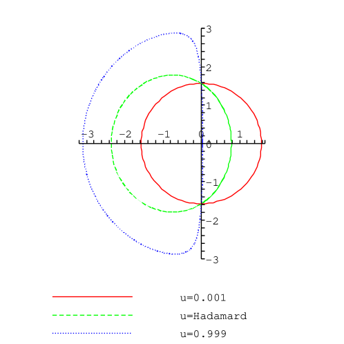
Figure 1: (Color online) The dependence on $u$ of shape of the orbit. Three cases $u\simeq 0$, $u=1/\sqrt{2}$ (the Hadamard matrix), and $u\simeq 1$ are shown.

III.3 Curvilinear integration along the orbit

Now we consider the integration with respect to $k$ on $[-\pi,\pi)$, which is necessary to calculate the expectations (12). The above result implies that this integration corresponds to the integration over $\gamma\in[-\pi,\pi)$, which performs the curvilinear integration along the orbit. We write the Jacobian associated with the map $k\to\gamma$ as $J=|dk/d\gamma|$. By simple calculation, we have (see Appendix A),

$$J=\frac{\sqrt{1-u^{2}}}{1-u^{2}\sin^{2}\gamma},$$ (33)

and the relation

$$\int_{-\pi}^{\pi}\frac{dk}{2\pi}f(k)=\int_{-\pi}^{\pi}\frac{d\gamma}{2\pi}\frac{\sqrt{1-u^{2}}}{1-u^{2}\sin^{2}\gamma}f(k(\gamma))$$ (34)

is established, where $k(\gamma)$ is determined by (41) and (42).

Then we change the variable as

$$\gamma\to y\quad;\quad y=u\sin\gamma,$$ (35)

to have the equality

$$\int_{-\pi}^{\pi}\frac{dk}{2\pi}f(k)=2\int_{-u}^{u}\frac{dy}{2\pi}\frac{1}{\sqrt{u^{2}-y^{2}}}\frac{\sqrt{1-u^{2}}}{1-y^{2}}f(k(y)).$$

That is, we arrive at the formula

$$\int_{-\pi}^{\pi}\frac{dk}{2\pi}f(k)=\int_{-u}^{u}dy\,\mu(y;u)f(k(y))$$

with Konno’s function (14).

IV LIMIT THEOREM OF QUANTUM WALKS

IV.1 Quantum walk starting from the origin

We assume that the quantum walk starts from $x=0$, that is

$$\Psi_{0}(x)=\delta(x)\left(\matrix{\alpha\cr\beta}\right)\quad\Leftrightarrow\quad\hat{\Psi}_{0}(k)=\left(\matrix{\alpha\cr\beta}\right),$$

where $\alpha,\beta\in{\bf C}$ with $|\alpha|^{2}+|\beta|^{2}=1$. We can express this initial wave function $\hat{\Psi}_{0}(k)$ as a linear combination of the two eigenfunctions (25) of the Hamiltonian ${\cal H}({\bf p})$ with ${\bf p}={\bf q}(k)$ in the way

$$\hat{\Psi}_{0}(k)=C_{+}(\hat{{\bf q}}(k))\psi_{+}(\hat{{\bf q}}(k))+C_{-}(\hat{{\bf q}}(k))\psi_{-}(\hat{{\bf q}}(k)),$$ (36)

where $C_{+}(\hat{{\bf p}})$ and $C_{-}(\hat{{\bf p}})$ are given as functions of $\hat{{\bf p}}={\bf p}/|{\bf p}|$ by (43) in Appendix B. Then, for $n=0,1,2,\cdots$, (23) gives

$$\hat{\Psi}_{n}(k) = e^{-i{\cal H}({\bf q}(k))n}$$ (37)

$$\times\Bigg{\{}C_{+}(\hat{{\bf q}}(k))\psi_{+}(\hat{{\bf q}}(k))+C_{-}(\hat{{\bf q}}(k))\psi_{-}(\hat{{\bf q}}(k))\Bigg{\}}$$

$$= e^{-iq(k)n}C_{+}(\hat{{\bf q}}(k))\psi_{+}(\hat{{\bf q}}(k))$$

$$\qquad\qquad+e^{iq(k)n}C_{-}(\hat{{\bf q}}(k))\psi_{-}(\hat{{\bf q}}(k)),$$

since $\psi_{\pm}(\hat{{\bf p}})$ are eigenfunctions of ${\cal H}({\bf p})$ with the eigenvalues $\lambda=\pm p$. It should be noted that the time dependence and the initial-qubit dependence are separately controlled by the absolute value of the vector ${\bf q}(k)$, $q(k)=|{\bf q}(k)|$, and by its direction, $\hat{{\bf q}}(k)$, respectively.

IV.2 Weak limit theorem

We recall the formula (12). It is enough to consider the case $f(x)=x^{r},r=0,1,2,\cdots.$ Following the argument by Grimmett et al. GJS04 , we find from (37),

$$\left(i\frac{d}{dk}\right)^{r}\hat{\Psi}_{n}(k) = \left(\frac{dq(k)}{dk}\right)^{r}e^{-iq(k)n}C_{+}(\hat{{\bf q}}(k))\psi_{+}(\hat{{\bf q}}(k))n^{r}$$ (38)

$$+ \left(-\frac{dq(k)}{dk}\right)^{r}e^{iq(k)n}C_{-}(\hat{{\bf q}}(k))\psi_{-}(\hat{{\bf q}}(k))n^{r}+{\cal O}(n^{r-1}).$$

Insert (37) and (38) in the formula (12), use the orthonormality (26), and take the limit $n\to\infty$. Then we have GJS04 ,

$$\lim_{n\to\infty}\langle(X_{n}/n)^{r}\rangle\\ =\int_{-\pi}^{\pi}\frac{dk}{2\pi}\Bigg{\{}|C_{+}(\hat{{\bf q}}(k))|^{2}+(-1)^{r}|C_{-}(\hat{{\bf q}}(k))|^{2}\Bigg{\}}\left(\frac{\sin(k+\theta)}{\sqrt{1/u^{2}-\cos^{2}(k+\theta)}}\right)^{r},$$

where we used (40).

Now we perform the map $k\to\gamma$. By (30), (34) and (44), we have

$$\lim_{n\to\infty}\langle(X_{n}/n)^{2m}\rangle = \int_{-\pi}^{\pi}\frac{d\gamma}{2\pi}\frac{\sqrt{1-u^{2}}}{1-u^{2}\sin^{2}\gamma}(u\sin\gamma)^{2m},$$

$$\lim_{n\to\infty}\langle(X_{n}/n)^{2m+1}\rangle = -\left\{(|\alpha|^{2}-|\beta|^{2})+\frac{\sqrt{1-u^{2}}}{u}(\alpha\beta^{*}e^{-i(\phi-\theta)}+\alpha^{*}\beta e^{i(\phi-\theta)})\right\}$$

$$\qquad\times\int_{-\pi}^{\pi}\frac{d\gamma}{2\pi}\frac{\sqrt{1-u^{2}}}{1-u^{2}\sin^{2}\gamma}(u\sin\gamma)^{2m+2}$$

for $m=0,1,2,\cdots$. Then we change the variable as (35). The results are expressed using (14) as

$$\lim_{n\to\infty}\langle(X_{n}/n)^{2m}\rangle = \int_{-u}^{u}dy\,\mu(y;u)y^{2m},$$

$$\lim_{n\to\infty}\langle(X_{n}/n)^{2m+1}\rangle = -\left\{(|\alpha|^{2}-|\beta|^{2})+\frac{\sqrt{1-u^{2}}}{u}(\alpha\beta^{*}e^{-i(\phi-\theta)}+\alpha^{*}\beta e^{i(\phi-\theta)})\right\}\int_{-u}^{u}dy\,\mu(y;u)y^{2m+2}.$$ (39)

Then we have arrived at the following limit theorem, which was first obtained by Konno Konno02a ; Konno02b .

Theorem  Let $X_{n}$ be the one-dimensional quantum walk associated with the matrix

$$A = \left(\matrix{a&b\cr-b^{*}&a^{*}}\right)$$

with $a,b\in{\bf C},|a|^{2}+|b|^{2}=1$, which starts from the state

$$\Psi_{0}(x)=\delta(x)\left(\matrix{\alpha\cr\beta}\right),\quad|\alpha|^{2}+|\beta|^{2}=1,\quad\alpha,\beta\in{\bf C}.$$

Then for any analytic function $f(x)$ on ${\bf Z}$,

$$\langle f(X_{n}/n)\rangle\quad\to\quad\int_{-\infty}^{\infty}dy\,f(y)\nu(y)\quad\mbox{in}\quad n\to\infty,$$

where $\nu(y)$ is given by (13)-(15).

V CONCLUDING REMARKS

We remark that the quantity $h=\mbox{\boldmath$\sigma$}\cdot\hat{{\bf p}}$ is called the helicity. The energy-momentum eigenfunctions $\psi_{+}({\bf p})$ and $\psi_{-}({\bf p})$ are also the eigenfunctions of the helicity with the eigenvalues $+1$ and $-1$, respectively. The difference between the behaviors of even moments and odd moments in (39) comes from the fact that these two states with opposite helicity contribute with the same sign to even moments and with alternating signs to odd moments, respectively, as we can see in (IV.2). In the quantum spin systems, the term of the form $\mbox{\boldmath$\sigma$}\cdot{\bf H}$ and $\mbox{\boldmath$\sigma$}\cdot{\bf d}$ appear in Hamiltonian, representing the Zeeman interaction between a spin and an external magnetic field ${\bf H}$, and the spin-orbit interaction with an anisotropy vector ${\bf d}$, respectively. We expect that these analogue with other physical systems will be useful, when we consider many-body systems of quantum walkers in the future.

The present one-dimensional quantum walks make a family of models, each of which is specified by a $2\times 2$ unitary matrix. The corresponding family of orbital states in the three-dimensional momentum space studied in this paper can be regarded as a geometrical representation of the unitary group ${\rm U}(2)$. This point of view will provide a useful sight in quantum-walk problems not only in solving problems but also in setting problems themselves and in classifying results. For example, what kind of quantum random walk models can be associated with the unitary group ${\rm SU}(3)$, in which the so-called Gell-Mann’s eight matrices (see, for example, Geo99 ) play the similar role to the Pauli matrices in ${\rm SU}(2)$ ? In the recent papers, a lot of interesting phenomena have been reported in a variety of quantum random walk models, which are associated with $3\times 3$ or larger matrices IKK04 ; IK05 ; VBBB05 . Symmetry and invariance, which are sometimes hidden in a variety of phenomena observed in quantum walks, should be clarified using the group-theoretical investigation in the future.

Appendix A ON THE ORBITS

Here we assume that $k+\theta\in[-\pi,\pi)$ for simplicity of description. By (18), we can see that

$$(i) q(k)=\pi-\arccos u\searrow\frac{\pi}{2}\searrow\arccos u\quad\mbox{as}\quad k+\theta=-\pi\nearrow-\frac{\pi}{2}\nearrow 0,$$

$$(ii) q(k)=\arccos u\nearrow\frac{\pi}{2}\nearrow\pi-\arccos u\quad\mbox{as}\quad k+\theta=0\nearrow\frac{\pi}{2}\nearrow\pi,$$

where $x=a\nearrow b$ (resp. $x=a\searrow b$) means the variable $x$ monotonically increases (resp. decreases) from $a$ to $b$. That is, $dq(k)/dk\leq 0$, when $-\pi\leq k+\theta\leq 0$, and $dq(k)/dk\geq 0$, when $0\leq k+\theta<-\pi$. By this observation and the general formula $(d/dx)\arccos x=\mp 1/\sqrt{1-x^{2}}$, we can determine the derivative as

$$\frac{dq(k)}{dk}=\frac{\sin(k+\theta)}{\sqrt{1/u^{2}-\cos^{2}(k+\theta)}}.$$ (40)

The equations (18)-(20) give

$${\bf q}(-\pi-\theta) = q_{\rm max}\Big{(}\sin(\phi-\theta),\cos(\phi-\theta),0\Big{)},$$

$${\bf q}(-\pi/2-\theta) = \frac{\pi}{2}\Big{(}\sqrt{1-u^{2}}\cos(\phi-\theta),-\sqrt{1-u^{2}}\sin(\phi-\theta),u\Big{)},$$

$${\bf q}(-\theta) = -q_{\rm min}\Big{(}\sin(\phi-\theta),\cos(\phi-\theta),0\Big{)},$$

$${\bf q}(\pi/2-\theta) = \frac{\pi}{2}\Big{(}-\sqrt{1-u^{2}}\cos(\phi-\theta),\sqrt{1-u^{2}}\sin(\phi-\theta),-u\Big{)},$$

where $q_{\rm min}=\arccos u$ and $q_{\rm max}=\pi-q_{\rm min}$.

The relations (29) and (30) imply

$$k+\theta=-\pi\quad \Leftrightarrow \quad\gamma=-\pi,$$

$$k+\theta=-\pi/2\quad \Leftrightarrow \quad\gamma=\pi/2,$$

$$k+\theta=0\quad \Leftrightarrow \quad\gamma=0,$$

$$k+\theta=\pi/2\quad \Leftrightarrow \quad\gamma=-\pi/2,$$

and they can be inverted as

$$\sin(k+\theta) = -\frac{(\sqrt{1-u^{2}}/u)\sin\gamma}{\sqrt{(1-u^{2})/u^{2}+\cos^{2}\gamma}},$$ (41)

$$\cos(k+\theta) = \frac{(1/u)\cos\gamma}{\sqrt{(1-u^{2})/u^{2}+\cos^{2}\gamma}}.$$ (42)

By differentiate the both sides of (42), we have

$$-\sin(k+\theta)dk=\frac{d}{d\gamma}\left[\frac{(1/u)\cos\gamma}{\sqrt{(1-u^{2})/u^{2}+\cos^{2}\gamma}}\right]d\gamma.$$

Here we see

$$\frac{d}{d\gamma}\left[\frac{(1/u)\cos\gamma}{\sqrt{(1-u^{2})/u^{2}+\cos^{2}\gamma}}\right]=\sin(k+\theta)\frac{\sqrt{1-u^{2}}}{1-u^{2}\sin^{2}\gamma},$$

where we have used (41). Then the Jacobian $J=|dk/d\gamma|$ is determined as (33).

Appendix B INITIAL STATE DEPENDENCE

Here we consider a two-component unit vector

$$\phi_{0}=\left(\matrix{\alpha\cr\beta}\right),\qquad\alpha,\beta\in{\bf C},\quad|\alpha|^{2}+|\beta|^{2}=1.$$

This can be represented as a linear combination of the two eigenfunctions of ${\cal H}({\bf p})=\mbox{\boldmath$\sigma$}\cdot{\bf p}$ given by (25) as

$$\phi_{0}=C_{+}(\hat{{\bf p}})\psi_{+}(\hat{{\bf p}})+C_{-}(\hat{{\bf p}})\psi_{-}(\hat{{\bf p}}),$$

where

$$C_{+}(\hat{{\bf p}}) = \psi_{+}^{\dagger}(\hat{{\bf p}})\phi_{0}=\alpha\cos\frac{\theta_{p}}{2}+\beta\sin\frac{\theta_{p}}{2}e^{-i\varphi_{p}},$$

$$C_{-}(\hat{{\bf p}}) = \psi_{-}^{\dagger}(\hat{{\bf p}})\phi_{0}=-\alpha\sin\frac{\theta_{p}}{2}e^{i\varphi_{p}}+\beta\cos\frac{\theta_{p}}{2}$$ (43)

by the orthonormality (26). By straightforward calculation we find

$$|C_{\pm}(\hat{{\bf p}})|^{2}=\frac{1}{2}\pm\frac{1}{2}\Bigg{\{}(|\alpha|^{2}-|\beta|^{2})\hat{p}_{3}+\alpha\beta^{*}(\hat{p}_{1}+i\hat{p}_{2})+\alpha^{*}\beta(\hat{p}_{1}-i\hat{p}_{2})\Bigg{\}}.$$

Now we set $\hat{{\bf p}}\Rightarrow\hat{{\bf q}}(\gamma)$, which is given by (32). Since

$$\hat{p}_{1}\pm i\hat{p}_{2}\quad\Rightarrow\quad\hat{q}_{1}\pm i\hat{q}_{2}=\Big{(}\sqrt{1-u^{2}}\sin\gamma\mp i\cos\gamma\Big{)}e^{\mp i(\phi-\theta)},$$

the above results become

$$|C_{\pm}(\hat{{\bf q}}(\gamma))|^{2} = \frac{1}{2}\pm\frac{1}{2}\Big{\{}(|\alpha|^{2}-|\beta|^{2})+\frac{\sqrt{1-u^{2}}}{u}(\alpha\beta^{*}e^{-i(\phi-\theta)}+\alpha^{*}\beta e^{i(\phi-\theta)}\Big{\}}u\sin\gamma$$ (44)

$$\mp\frac{1}{2}i(\alpha\beta^{*}e^{-i(\phi-\theta)}-\alpha^{*}\beta e^{i(\phi-\theta)})\cos\gamma.$$

- (1) Y. Aharonov, L. Davidovich, and N. Zagury, Phys. Rev. A 48, 1687 (1993).
- (2) D. A. Meyer, J. Stat. Phys. 85, 551 (1996).
- (3) A. Nayak and A. Vishwanath, Quantum walk on the line, e-print quant-ph/0010117.
- (4) A. Ambainis, E. Bach, A. Nayak, A. Vishwanath, and J. Watrous, in Proceedings of the 33rd Annual ACM Symposium on Theory of Computing (ACM Press, New York, 2001), pp.37-49.
- (5) J. Kempe, Contemp. Phys. 44, 307 (2003).
- (6) B. Tregenna, W. Flanagan, W. Maile, and V. Kendon, New J. Phys. 5, 83 (2003).
- (7) A. Ambainis, Int. J. Quantum Inform. 1, 507 (2003).
- (8) N. Konno, Quantum Inf. Process. 1, 345 (2002).
- (9) N. Konno, A new type of limit theorems for the one-dimensional quantum random walk, to be published in J. Math. Soc. Jpn.; e-print quant-ph/0206103.
- (10) G. Grimmett, S. Janson, and P. F. Scudo, Phys. Rev. E 69, 026119 (2004).
- (11) T. Oka, N. Konno, R. Arita, and H. Aoki, Phys. Rev. Lett. 94, 100602 (2005).
- (12) N. Konno, Limit theorems and absorption problems for one-dimensional correlated random walks, e-print quant-ph/0310191.
- (13) H. Weyl, Z. Physik 56, 330 (1929).
- (14) J. D. Bjorken and S. D. Drell, Relativistic Quantum Mechanics (McGraw-Hill, New York, 1964).
- (15) C. Itzykson and J-B. Zuber, Quantum Field Theory (McGraw-Hill, New York, 1980).
- (16) H. Georgi, Lie Algebras in Particle Physics, 2nd ed. (Perseus Books, Reading, 1999).
- (17) N. Inui, Y. Konishi, and N. Konno, Phys. Rev. A 69, 052323 (2004).
- (18) N. Inui and N. Konno, Localization of multi-state quantum walk in one dimension, Physica A (2005) (in press); e-print quant-ph/0403153.
- (19) S. E. Venegas-Andraca, J. L. Ball, K. Burnett, and S. Bose, Quantum walks with entangled coins, e-print quant-ph/0411151.