A new local invariant for quantum gates

Abstract

In this paper we study the properties of two-qubit gates. We review the most common parameterizations for the local equivalence classes of two-qubit gates and the connections between them. We then introduce a new discrete local invariant, namely the number of local degrees of freedom that a gate can bind. The value of this invariant is calculated analytically for all the local equivalence classes of two-qubit gates. We find that almost all two-qubit gates can bind the full six local degrees of freedom and are in this sense more effective than the controlled-NOT gate which only can bind four local degrees of freedom.

I Introduction

Quantum computation is a novel information processing method in which classical information is encoded into a quantum-mechanical system Nielsen and Chuang (2000), called the quantum register. In most quantum computers the quantum register is a collection of two-level systems, termed qubits. The computation is performed by the unitary temporal evolution of the register, followed by a measurement. In order to execute a quantum algorithm, one has to be able to generate the required unitary propagators that are usually referred to as quantum gates.

It has been shown that almost any fixed two-qubit gate together with arbitrary single-qubit gates is universal Deutsch et al. (1995); Lloyd (1995), i.e., any $n$-qubit gate may be constructed using only a finite number of these gates. Conventionally, the elementary gate library is chosen to consist of the single-qubit rotations $R_{x},R_{y},R_{z}$ and the controlled-NOT gate (CNOT). However, in many realizations, the CNOT is not the natural choice for the entangling two-qubit gate. Recently, an optimal construction of an arbitrary two-qubit gate using three CNOTs and 15 single-qubit rotations has been introduced Shende et al. (2004a). In addition, constructions for the double-CNOT (DCNOT) Zhang et al. (2004a), the controlled-unitary gates Zhang et al. (2004a) and the so-called super controlled gates Ye et al. (2004) have been published. A construction using only two applications of the $B$ gate has been introduced in Ref. Zhang et al. (2004b), and in Ref. Zhang et al. (2004c) it is shown that no other construction using only two applications of a fixed two-qubit gate exists. Extensions to the $n$-qubit case are mainly uninvestigated. However, several CNOT-based constructions with $O(4^{n})$ asymptotic behaviour exist, the best of which Shende et al. (2004b); Bergholm et al. (2004) have CNOT counts of twice the highest known lower bound Shende et al. (2004a).

In many of the proposed realizations for quantum computers the individual qubits are fully controllable, whereas the interqubit interactions are often fixed. In addition, single-qubit operations tend to be considerably faster to implement than multiqubit operations. This is why it often makes sense to study the local equivalence classes of multiqubit gates instead of the gates themselves. Two gates are considered equivalent if they can be converted to each other using only local operations, i.e., tensor products of single-qubit gates. The equivalence classes are characterized by local invariants, which are quantities that are not affected by local operations.

In this paper we briefly review the currently used parameterizations for the local equivalence classes of two-qubit gates and point out their equivalence. We then introduce a new discrete local invariant which describes the number of local degrees of freedom a gate can bind. Finally, we calculate the value of this invariant for all the local equivalence classes of two-qubit gates.

II Local equivalence classes of two-qubit gates

An $n$-qubit quantum gate $k$ is said to be local iff it consists solely of single-qubit rotations: $k\in SU(2)^{\otimes n}=:\mathbb{L}_{n}$. Two $n$-qubit gates $U_{1},U_{2}\in SU(2^{n})$ are said to be locally equivalent iff $U_{2}=k_{1}U_{1}k_{2}$, where $k_{1},k_{2}\in\mathbb{L}_{n}$. This constitutes an equivalence relation, which we denote by $U_{1}\sim U_{2}$.

Using the theory of Lie groups it can be shown Khaneja et al. (2001); Zhang et al. (2003) that any two-qubit gate $U\in SU(4)$ can be decomposed using the Cartan decomposition as

$$U=k_{1}Ak_{2}=k_{1}\exp\left(\frac{i}{2}(c_{1}\sigma_{x}\otimes\sigma_{x}+c_{2}\sigma_{y}\otimes\sigma_{y}+c_{3}\sigma_{z}\otimes\sigma_{z})\right)k_{2},$$ (1)

where $\sigma_{i}$ denote the Pauli matrices, $k_{1},k_{2}\in\mathbb{L}_{2}$ and $c_{1},c_{2},c_{3}\in\mathbb{R}$. The matrix $A$ is a member of the Cartan subgroup of the decomposition and carries all the nonlocal properties of the gate $U$. Hence the local equivalence classes of two-qubit gates can be parameterized by the three scalars $[c_{1},c_{2},c_{3}]$, known as canonical parameters. This is a minimal set of parameters since the group $SU(4)$ is 15-dimensional and the local rotations eliminate $2\times\text{dim}(SU(2)^{\otimes 2})=12$ degrees of freedom thereof. The canonical parameterization is visualized in Fig. 1. The tetrahedron $OA_{1}A_{2}A_{3}$ in the figure is called a Weyl chamber. It is defined by the inequalities $\pi\geq c_{1}\geq c_{2}\geq c_{3}\geq 0,\pi-c_{1}\geq c_{2}$. The Weyl chamber contains all the local equivalence classes of two-qubit gates exactly once, excepting the fact that the triangles $LA_{1}A_{2}$ and $LOA_{2}$ are equivalent.

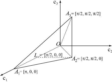
Figure 1: Weyl chamber. Points $O$ and $A_{1}$ correspond to the identity gate $I$, $A_{3}$ to the SWAP gate, $L$ to the controlled-NOT gate (CNOT) and $A_{2}$ to the double controlled-NOT gate (DCNOT) Zhang et al. (2003).

The matrix

$$Q=\frac{1}{\sqrt{2}}\begin{pmatrix}1&0&0&1\\ 0&-i&-i&0\\ 0&1&-1&0\\ -i&0&0&i\end{pmatrix}$$ (2)

is the transformation from the standard basis of states $\{\left|00\right\rangle,\,\left|01\right\rangle,\,\left|10\right\rangle,\,\left|11\right\rangle\}$ into the Bell basis, also known as the magic basis Makhlin (2002). We use the lower index $B$ to denote the change of basis: $U_{B}:=QUQ^{\dagger}$. The magic basis has the special property that local gates expressed in it are orthogonal. In other words, conjugation by $Q$ is a group isomorphism between $SU(2)\otimes SU(2)$ and $SO(4)$. Furthermore, it renders our chosen Cartan subgroup (generated by $\sigma_{x}\otimes\sigma_{x}$, $\sigma_{y}\otimes\sigma_{y}$ and $\sigma_{z}\otimes\sigma_{z}$) diagonal. These two properties enable us to calculate the canonical parameters of any given $SU(4)$ gate $U=k_{1}Ak_{2}$. The parameters are obtained from the spectrum of the matrix $M(U):=U_{B}^{T}U_{B}$ which is given by

$$\lambda\left(M(U)\right)=\left\{e^{i(c_{1}+c_{2}-c_{3})},e^{i(c_{1}-c_{2}+c_{3})},e^{i(-c_{1}+c_{2}+c_{3})},e^{-i(c_{1}+c_{2}+c_{3})}\right\}.$$ (3)

Ref. Childs et al. (2003) presents an algorithm for extracting the canonical parameters $c_{i}$ from this spectrum in a convenient way although it uses a slightly different notation. The equivalence of the methods becomes apparent using the equality $Q^{T}Q=-\sigma_{y}\otimes\sigma_{y}$, since

$$\lambda\left(M(U)\right)=\lambda\left((QUQ^{\dagger})^{T}QUQ^{\dagger}\right)=\lambda\left((\sigma_{y}\otimes\sigma_{y})^{\dagger}U^{T}(\sigma_{y}\otimes\sigma_{y})U\right)=\lambda\left(U(\sigma_{y}\otimes\sigma_{y})U^{T}(\sigma_{y}\otimes\sigma_{y})\right)=\lambda(U\tilde{U}).$$ (4)

Ref. Shende et al. (2004a) presents another system of invariants, namely the characteristic polynomials $\chi[\gamma_{2}(U)]$, where $\gamma_{2}(U)=U(\sigma_{y}\otimes\sigma_{y})U^{T}(\sigma_{y}\otimes\sigma_{y})$. They are completely equivalent to the canonical parameters since the characteristic polynomial $\chi[\gamma_{2}(U)]$ carries exactly the same information as $\lambda\left(M(U)\right)=\lambda(\gamma_{2}(U))$.

Another useful parameterization for the two-qubit local equivalence classes is provided by the Makhlin invariants $G_{1}$ and $G_{2}$ Makhlin (2002). For a gate $U\in U(4)$, they are defined as

$$G_{1}=\frac{\operatorname{Tr}^{2}M(U)}{16\det U},\qquad G_{2}=\frac{\operatorname{Tr}^{2}M(U)-\operatorname{Tr}M(U)^{2}}{4\det U}.$$ (5)

The Makhlin invariants are by far the easiest ones to calculate. They, too, provide the same information as the previous invariants since $\lambda\left(M(U)\right)$ is fully determined by them. $G_{1}$ may be complex but $G_{2}$ is always a real number, which leads to three real-valued invariants. If $U$ is represented as in Eq. (1), the Makhlin invariants reduce to Zhang et al. (2003)

$$g_{1} :=\mathrm{Re}\,G_{1}=\cos^{2}c_{1}\cos^{2}c_{2}\cos^{2}c_{3}-\sin^{2}c_{1}\sin^{2}c_{2}\sin^{2}c_{3},$$

$$g_{2} :=\mathrm{Im}\,G_{1}=\frac{1}{4}\sin 2c_{1}\sin 2c_{2}\sin 2c_{3},$$ (6)

$$g_{3} :=G_{2}=4\cos^{2}c_{1}\cos^{2}c_{2}\cos^{2}c_{3}-4\sin^{2}c_{1}\sin^{2}c_{2}\sin^{2}c_{3}-\cos 2c_{1}\cos 2c_{2}\cos 2c_{3}.$$

Example values of the invariants of different gates are given in Table 1. The set of all the two-qubit gate equivalence classes in the Makhlin parameter space is presented in Fig. 2. The surface is given by the equations

$$g_{1} =\cos^{2}s\cos^{4}t-\sin^{2}s\sin^{4}t$$

$$g_{2} =\frac{1}{4}\sin(2s)\sin^{2}(2t)$$ (7)

$$g_{3} =4g_{1}-\cos(2s)\cos^{2}(2t),$$

where $s\in[0,\pi],\,t\in[0,\pi/2]$. The surface and the inside of the object correspond to the surface and the inside of the Weyl chamber, respectively.

Gate	$c_{1}$	$c_{2}$	$c_{3}$	$g_{1}$	$g_{2}$	$g_{3}$
$I$	0	0	0	1	0	3
SWAP	$\frac{\pi}{2}$	$\frac{\pi}{2}$	$\frac{\pi}{2}$	-1	0	-3
CNOT	$\frac{\pi}{2}$	0	0	0	0	1
DCNOT	$\frac{\pi}{2}$	$\frac{\pi}{2}$	0	0	0	-1
$\sqrt{\text{SWAP}}$	$\frac{\pi}{4}$	$\frac{\pi}{4}$	$\frac{\pi}{4}$	0	$\frac{1}{4}$	0
$\sqrt{\text{SWAP}}^{\,-1}$	$\frac{3\pi}{4}$	$\frac{\pi}{4}$	$\frac{\pi}{4}$	0	-$\frac{1}{4}$	0
B	$\frac{\pi}{2}$	$\frac{\pi}{4}$	0	0	0	0
controlled-U	$\alpha$	0	0	$\cos^{2}(\alpha)$	0	$2\cos^{2}(\alpha)+1$
SPE	$\frac{\pi}{2}$	$\alpha$	0	0	0	$\cos(2\alpha)$

Table 1: Values of the canonical and Makhlin invariants for some common gates. SPE denotes a special perfect entangler Rezakhani (2004); Ye et al. (2004).

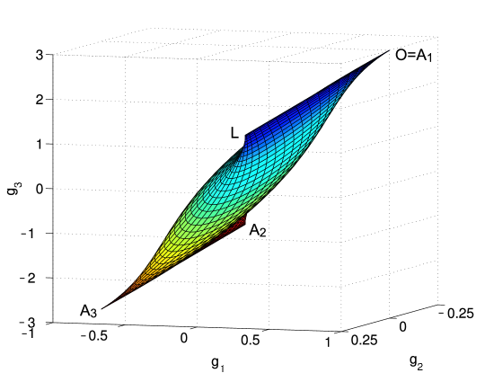
Figure 2: Weyl chamber in the coordinates of the Makhlin invariants.

III The local invariant $\eta$

Let us use

$$L^{k}_{n}(\mathbf{a},\vec{\theta}):=\exp\left(\sum_{j=1}^{3n}a_{j}(\vec{\theta})X_{j}\right),\qquad L^{k}_{n}(\mathbf{a},\vec{\theta})\in\mathbb{L}_{n}\quad\forall\vec{\theta}\in\mathbb{R}^{k},$$ (8)

where $j$ runs over the $3n$ local generators of $SU(2^{n})$, to denote a $k$-parameter family of $n$-qubit local gates. It is defined by the function $\mathbf{a}:\mathbb{R}^{k}\to\mathbb{R}^{3n}$. The generators $X_{j}$ are normalized such that they are orthonormal with respect to the inner product $\left\langle X,Y\right\rangle:=\operatorname{Tr}\left(X^{\dagger}Y\right)$.

A gate $U\in SU(2^{n})$ is said to leak $k$ local degrees of freedom iff there exist nondegenerate functions $\mathbf{a}$ and $\mathbf{b}$ such that

$$UL^{k}_{n}(\mathbf{a},\vec{\theta})=L^{k}_{n}(\mathbf{b},\vec{\theta})U\quad\forall\vec{\theta}\in\mathbb{R}^{k}.$$ (9)

A gate binds the local degrees of freedom that it does not leak. We define a function $\eta$ : $SU(2^{n})\to\mathbb{N}$ to indicate the number of local degrees of freedom that an $n$-qubit gate $U$ binds. We always have $\max\eta\leq 3n$, i.e., at most three degrees of freedom for each qubit.

Assume now that the functions $\mathbf{a}$ and $\mathbf{b}$ satisfy Eq. (9) for the gate $U$. For a gate $V=k_{1}Uk_{2}$, where $k_{1},k_{2}\in\mathbb{L}_{n}$, we obtain

$$V\>\left[k_{2}^{\dagger}L^{k}_{n}(\mathbf{a},\vec{\theta})k_{2}\right]=k_{1}Uk_{2}\>k_{2}^{\dagger}L^{k}_{n}(\mathbf{a},\vec{\theta})k_{2}=k_{1}L^{k}_{n}(\mathbf{b},\vec{\theta})\>Uk_{2}=\left[k_{1}L^{k}_{n}(\mathbf{b},\vec{\theta})k_{1}^{\dagger}\right]\>V.$$ (10)

We also have

$$k_{1}L^{k}_{n}(\mathbf{b},\vec{\theta})k_{1}^{\dagger}=\exp\left(\sum_{j=1}^{3n}b_{j}(\vec{\theta})\operatorname{Ad}(k_{1})X_{j}\right)=\exp\left(\sum_{j=1}^{3n}\tilde{b}_{j}(\vec{\theta})X_{j}\right)=L^{k}_{n}(\tilde{\mathbf{b}},\vec{\theta}),$$ (11)

since $\operatorname{Ad}(g)$ is a linear bijection and $k_{1}$ is a local gate. If $\mathbf{b}$ is nondegenerate then so is $\tilde{\mathbf{b}}$. A similar argument naturally holds for $k_{2}^{\dagger}L^{k}_{n}(\mathbf{a},\vec{\theta})k_{2}$, which yields $VL^{k}_{n}(\tilde{\mathbf{a}},\vec{\theta})L^{k}_{n}(\tilde{\mathbf{b}},\vec{\theta})V$ and proves that $\eta$ is indeed a local invariant.

Equation (9) is equivalent to

$$U\exp\left(\sum_{j=1}^{3n}a_{j}(\vec{\theta})X_{j}\right)U^{\dagger}=\exp\left(\sum_{j=1}^{3n}a_{j}(\vec{\theta})\operatorname{Ad}(U)X_{j}\right)=\exp\left(\sum_{k=1}^{3n}b_{k}(\vec{\theta})X_{k}\right)$$ (12)

This is fulfilled if

$$\sum_{j=1}^{3n}a_{j}(\vec{\theta})\operatorname{Ad}(U)X_{j}=\sum_{k=1}^{3n}b_{k}(\vec{\theta})X_{k}.$$ (13)

Now, as we take a sidewise inner product $\langle\cdot,X_{i}\rangle$ with each of the $4^{n}-1$ generators of $SU(2^{n})$, we obtain equivalently

$$\sum_{j=1}^{3n}W_{ij}a_{j}(\vec{\theta})=\sum_{k=1}^{3n}b_{k}(\vec{\theta})\delta_{ki},\qquad i=1,2,\ldots,4^{n}-1,$$ (14)

where $W_{ij}=\operatorname{Tr}\left(UX_{j}^{\dagger}U^{\dagger}X_{i}\right)$. The generators $X_{j}$ are antihermitian and $U$ is unitary. This implies that the elements $W_{ij}$ are real. Written in matrix form this is

$$W\mathbf{a}(\vec{\theta})=\begin{pmatrix}W_{L}\\ W_{N}\end{pmatrix}\mathbf{a}(\vec{\theta})=\begin{pmatrix}\mathbf{b}(\vec{\theta})\\ \vec{0}\end{pmatrix}\quad\forall\vec{\theta}\in\mathbb{R}^{k},$$ (15)

where $W_{L}\in\mathbb{R}^{3n\times 3n}$, $W_{N}\in\mathbb{R}^{(4^{n}-1-3n)\times 3n}$ and the indices $L$ and $N$ stand for local and nonlocal, respectively. Hence, we must have $\mathbf{a}(\vec{\theta})\in\ker{W_{N}}$ for all values of $\vec{\theta}$. Moreover, since $\mathbf{b}$ must have the same dimensionality as $\mathbf{a}$, the component of $\ker W_{N}$ parallel to $\ker W_{L}$ must be disregarded. Using the rank-nullity theorem we finally obtain

$$\eta(U)=3n-\dim(\ker W_{N})+\dim(\ker W_{L}\cap\ker W_{N}).$$ (16)

IV $\eta$ for two-qubit gates

For the set of two-qubit gates $U\in SU(4)$, $\max\eta\leq 6$. It is obvious that $\eta(\text{I})=0$ and $\eta(\text{SWAP})=0$ since all local gates and hence all local degrees of freedom may be commuted through these gates. It is also known that $\eta(\text{CNOT})=4$ and $\eta(\text{DCNOT})=4$. The result for CNOT is obtained by combining the commutation properties of CNOT with the Euler rotations $R_{z}$ and $R_{x}$ and the fact that an arbitrary two-qubit gate may be implemented using at most three CNOTs Shende et al. (2004a); Bullock and Markov (2003); Vidal and Dawson (2004); Vatan and Williams (2004). Similar arguments for the DCNOT are presented in Ref. Zhang et al. (2004a), including the explicit implementation of an arbitrary two-qubit gate using three DCNOTs. Also, from the construction of Ref. Zhang et al. (2004b), it is clear that $\eta(B)\geq 5$. Apart from such observations, no explicit calculations for $\eta$ have been presented in the literature so far.

We will now proceed to derive an analytical expression for $\eta$ for an arbitrary two-qubit gate. Because $\eta$ is a local invariant, it is enough to consider gates of the type

$$A=\exp\left(\frac{i}{2}(c_{1}\sigma_{x}\otimes\sigma_{x}+c_{2}\sigma_{y}\otimes\sigma_{y}+c_{3}\sigma_{z}\otimes\sigma_{z})\right)=\exp\bigg{(}\frac{i}{2}\begin{pmatrix}c_{3}&0&0&c_{1}-c_{2}\\ 0&-c_{3}&c_{1}+c_{2}&0\\ 0&c_{1}+c_{2}&-c_{3}&0\\ c_{1}-c_{2}&0&0&c_{3}\end{pmatrix}\bigg{)}$$ (17)

which represent all the nonlocal equivalence classes. The calculation of the elements of $W_{L}$ and $W_{N}$ is straightforward. Calculating the matrix exponential and simplifying the expression using elementary trigonometric identities results in

$$W_{L}=\begin{pmatrix}l^{1}_{1,1}&0&0&l^{1}_{1,2}&0&0\\ 0&l^{2}_{1,1}&0&0&l^{2}_{1,2}&0\\ 0&0&l^{3}_{1,1}&0&0&l^{3}_{1,2}\\ l^{1}_{2,1}&0&0&l^{1}_{2,2}&0&0\\ 0&l^{2}_{2,1}&0&0&l^{2}_{2,2}&0\\ 0&0&l^{3}_{2,1}&0&0&l^{3}_{2,2}\end{pmatrix},\qquad W_{N}=\begin{pmatrix}0&0&0&0&0&0\\ 0&0&n^{3}_{1,1}&0&0&n^{3}_{1,2}\\ 0&n^{2}_{1,1}&0&0&n^{2}_{1,2}&0\\ 0&0&n^{3}_{2,1}&0&0&n^{3}_{2,2}\\ 0&0&0&0&0&0\\ n^{1}_{1,1}&0&0&n^{1}_{1,2}&0&0\\ 0&n^{2}_{2,1}&0&0&n^{2}_{2,2}&0\\ n^{1}_{2,1}&0&0&n^{1}_{2,2}&0&0\\ 0&0&0&0&0&0\\ \end{pmatrix},$$ (18)

where the non-zero elements are

$$L^{1} :=\begin{pmatrix}l^{1}_{1,1}&l^{1}_{1,2}\\ l^{1}_{2,1}&l^{1}_{2,2}\end{pmatrix}=\begin{pmatrix}\cos c_{2}\cos c_{3}&\sin c_{2}\sin c_{3}\\ \sin c_{2}\sin c_{3}&\cos c_{2}\cos c_{3}\end{pmatrix},\qquad N^{1} :=\begin{pmatrix}n^{1}_{1,1}&n^{1}_{1,2}\\ n^{1}_{2,1}&n^{1}_{2,2}\end{pmatrix}=\begin{pmatrix}\sin c_{2}\cos c_{3}&-\cos c_{2}\sin c_{3}\\ -\cos c_{2}\sin c_{3}&\sin c_{2}\cos c_{3}\end{pmatrix},$$

$$L^{2} :=\begin{pmatrix}l^{2}_{1,1}&l^{2}_{1,2}\\ l^{2}_{2,1}&l^{2}_{2,2}\end{pmatrix}=\begin{pmatrix}\cos c_{1}\cos c_{3}&\sin c_{1}\sin c_{3}\\ \sin c_{1}\sin c_{3}&\cos c_{1}\cos c_{3}\end{pmatrix},\qquad N^{2} :=\begin{pmatrix}n^{2}_{1,1}&n^{2}_{1,2}\\ n^{2}_{2,1}&n^{2}_{2,2}\end{pmatrix}=\begin{pmatrix}-\sin c_{1}\cos c_{3}&\cos c_{1}\sin c_{3}\\ \cos c_{1}\sin c_{3}&-\sin c_{1}\cos c_{3}\end{pmatrix},$$

$$L^{3} :=\begin{pmatrix}l^{3}_{1,1}&l^{3}_{1,2}\\ l^{3}_{2,1}&l^{3}_{2,2}\end{pmatrix}=\begin{pmatrix}\cos c_{1}\cos c_{2}&\sin c_{1}\sin c_{2}\\ \sin c_{1}\sin c_{2}&\cos c_{1}\cos c_{2}\end{pmatrix},\qquad N^{3} :=\begin{pmatrix}n^{3}_{1,1}&n^{3}_{1,2}\\ n^{3}_{2,1}&n^{3}_{2,2}\end{pmatrix}=\begin{pmatrix}\sin c_{1}\cos c_{2}&-\cos c_{1}\sin c_{2}\\ -\cos c_{1}\sin c_{2}&\sin c_{1}\cos c_{2}\end{pmatrix}.$$ (19)

From Eqs. (18)–(IV) it is seen that Eq. (15) decomposes into six separate equations:

$$L^{i}\begin{pmatrix}a_{i}\\ a_{i+3}\end{pmatrix}=\begin{pmatrix}b_{i}\\ b_{i+3}\end{pmatrix},\qquad N^{i}\begin{pmatrix}a_{i}\\ a_{i+3}\end{pmatrix}=\begin{pmatrix}0\\ 0\end{pmatrix},\qquad i=1,2,3.$$ (20)

Each block $L^{i}$ produces a two-dimensional null space iff all the elements of $L^{i}$ equal zero. A one-dimensional null space is formed iff $\det L^{i}=\cos(c_{j}+c_{k})\cos(c_{j}-c_{k})=0$, where $\epsilon_{ijk}=1$, but $N^{i}\neq 0$. Similarly, each block $N^{i}$ produces a two-dimensional null space iff all the elements of $N^{i}$ equal zero, and a one-dimensional null space iff $\det N^{i}=(-1)^{i+1}\sin(c_{j}+c_{k})\sin(c_{j}-c_{k})=0$, where $\epsilon_{ijk}=1$, but $N^{i}\neq 0$.

Taking into account the correlations among the elements of the matrices $L^{i}$ and $N^{i}$ we find that in the two-qubit case $\ker W_{L}\cap\ker W_{N}=\{\vec{0}\}$ always. Thus we have $\eta=6-\dim(\ker W_{N})$ and the number of local degrees of freedom leaked is given by the nullity of $W_{N}$. The results for all the possible values of $[c_{1},c_{2},c_{3}]$ are collected in Table 2. One notices that everywhere inside the Weyl chamber $\eta$ reaches its maximum value of 6. At the vertices $O=A_{1}$ and $A_{3}$ $\eta=0$, on the edges between them $\eta=3$, on the edges $OA_{1},A_{2}A_{3}$ $\eta=4$ and on the faces $OA_{1}A_{3},OA_{2}A_{3},A_{1}A_{2}A_{3}$ $\eta=5$.

$[c_{1},c_{2},c_{3}]$	Set in the Weyl chamber	$\eta$
$[0,0,0]\stackrel{{\scriptstyle\wedge}}{{=}}[\pi,0,0]$	$O,A_{1}$	0
$[\pi/2,\pi/2,\pi/2]$	$A_{3}$	0
$[x,x,x],x\neq 0,x\neq\pi/2$	$OA_{3}\setminus\{O,A_{3}\}$	3
$[\pi-x,x,x],x\neq 0,x\neq\pi/2$	$A_{1}A_{3}\setminus\{A_{1},A_{3}\}$	3
$[x,0,0]\stackrel{{\scriptstyle\wedge}}{{=}}[\pi-x,0,0],x\neq 0$	$OA_{1}\setminus\{O,A_{1}\}$	4
$[\pi/2,\pi/2,x],x\neq\pi/2$	$A_{2}A_{3}\setminus\{A_{3}\}$	4
$[x,x,y],x\neq y,x\neq\pi/2$	$OA_{1}A_{3}\setminus\{OA_{3},A_{1}A_{3}\}$	5
$[x,y,y],x\neq y,x+y\neq\pi,y\neq 0$	$OA_{2}A_{3}\setminus\{OA_{3},A_{2}A_{3}\}$	5
$[\pi-x,x,y],x\neq y,x\neq\pi/2$	$A_{1}A_{2}A_{3}\setminus\{A_{1}A_{3},A_{2}A_{3}\}$	5
$\{$All other points$\}$	$\{$All other points$\}$	6

Table 2: $\eta$, or the number of local degrees of freedom bound, for the local equivalence classes of two-qubit gates.

The number of local degrees of freedom that the gate $U$ leaks is obtained as the number of pairs of equal eigenvalues $\lambda_{i}$ in the spectrum of the matrix $M(U)$, presented in Eq. (3). In other words, any $n$-fold eigenvalue of $M(U)$ indicates $n(n-1)/2$ local degrees of freedom that pass through the gate $U$. Translated to the language of the Weyl chamber, each Weyl symmetry plane the point $[c_{1},c_{2},c_{3}]$ touches causes the gate to leak one local degree of freedom.

V Conclusion

In this paper we have introduced a new local invariant $\eta$ for quantum gates, indicating the number of local degrees of freedom a gate can bind. Furthermore, we have analytically calculated the value of this invariant for all two-qubit gates. We have found that almost all two-qubit gates can bind the full six local degrees of freedom. However, most of the commonly occurring gates such as CNOT or $\sqrt{\text{SWAP}}$ are exceptions to the rule, performing much worse in this sense.

The meaning of $\eta$ is illustrated by considering the lower bounds on gate counts for a generic $n$-qubit circuit. Let the gate library consist of all one-qubit gates and a fixed two-qubit gate $U$. Then almost all $n$-qubit gates cannot be simulated with a circuit consisting of fewer than

$$N_{U}=\left\lceil\frac{4^{n}-3n-1}{\eta(U)}\right\rceil$$ (21)

applications of the two-qubit gate. This result is a straightforward generalization of Proposition III.1 in Ref. Shende et al. (2004a). The gates binding the full six degrees of freedom are thus expected to be the most efficient building blocks for multiqubit gates.

Appendix A Mathematical prerequisites

The Lie algebra $\mathfrak{g}$ of a linear Lie group $G<\text{GL}(n,\mathbb{K})$ is the set

$$\mathfrak{g}:=\{X\in\mathbb{K}^{n\times n}|\exp(tX)\in G\quad\forall t\in\mathbb{R}\}.$$ (22)

In can be shown that $\mathfrak{g}$ is a real vector space spanned by the generators of $G$. For example, the Lie algebra $\mathfrak{su}(n)$ of the group $\text{SU}(n)$ consists of all the $n\times n$ complex antihermitian traceless matrices.

The adjoint representation of a Lie group $G$, $\operatorname{Ad}:G\to\text{Aut}(\mathfrak{g})$, is a group homomorphism defined by

$$\operatorname{Ad}(g)X:=gXg^{-1}\quad(g\in G,X\in\mathfrak{g}).$$ (23)

It behaves in a rather simple way in exponentiation:

$$\exp\left(\operatorname{Ad}(g)X\right)=g\exp\left(X\right)g^{-1}\quad\text{for all }g\in G,\>X\in\mathfrak{g}.$$ (24)

Also, if we define an inner product $\left\langle X,Y\right\rangle:=\operatorname{Tr}\left(X^{\dagger}Y\right)$ for $\mathfrak{g}$, we find that it is preserved by the adjoint representation:

$$\left\langle\operatorname{Ad}(g)X,\operatorname{Ad}(g)Y\right\rangle=\left\langle X,Y\right\rangle\quad\text{for all }g\in G,\>X,Y\in\mathfrak{g}.$$ (25)

As a concrete example, the adjoint representation keeps orthonormal bases of $\mathfrak{g}$ orthonormal.

References

- Nielsen and Chuang (2000) M. A. Nielsen and I. L. Chuang, Quantum Computation and Quantum Information (Cambridge University Press, Cambridge, 2000).
- Deutsch et al. (1995) D. Deutsch, A. Barenco, and A. Ekert, Proc. R. Soc. London A 449, 669 (1995), eprint quant-ph/9505018.
- Lloyd (1995) S. Lloyd, Phys. Rev. Lett. 75, 346 (1995).
- Shende et al. (2004a) V. V. Shende, I. L. Markov, and S. S. Bullock, Phys. Rev. A 69, 062321 (2004a), eprint quant-ph/0308033.
- Zhang et al. (2004a) J. Zhang, J. Vala, S. Sastry, and K. B. Whaley, Phys. Rev. A 69, 042309 (2004a), eprint quant-ph/0308167.
- Ye et al. (2004) M.-Y. Ye, G.-C. Guo, and Y.-S. Zhang (2004), eprint quant-ph/0407108.
- Zhang et al. (2004b) J. Zhang, J. Vala, S. Sastry, and K. B. Whaley, Phys. Rev. Lett. 93, 020502 (2004b), eprint quant-ph/0312193.
- Zhang et al. (2004c) Y.-S. Zhang, M.-Y. Ye, and G.-C. Guo (2004c), eprint quant-ph/0411058.
- Shende et al. (2004b) V. V. Shende, S. S. Bullock, and I. L. Markov (2004b), eprint quant-ph/0406176.
- Bergholm et al. (2004) V. Bergholm, J. J. Vartiainen, M. Möttönen, and M. M. Salomaa (2004), eprint quant-ph/0410066.
- Khaneja et al. (2001) N. Khaneja, R. Brockett, and S. J. Glaser, Phys. Rev. A 63, 032308 (2001), eprint quant-ph/0006114.
- Zhang et al. (2003) J. Zhang, J. Vala, S. Sastry, and K. B. Whaley, Phys. Rev. A 67, 042313 (2003).
- Makhlin (2002) Y. Makhlin, Quantum Inf. Process. 1, 243 (2002), eprint quant-ph/0002045.
- Childs et al. (2003) A. M. Childs, H. L. Haselgrove, and M. A. Nielsen, Phys. Rev. A 68, 052311 (2003), eprint quant-ph/0307190.
- Rezakhani (2004) A. T. Rezakhani (2004), eprint quant-ph/0405046.
- Bullock and Markov (2003) S. S. Bullock and I. L. Markov, Phys. Rev. A 68, 0123318 (2003).
- Vidal and Dawson (2004) G. Vidal and C. M. Dawson, Phys. Rev. A 69, 010301 (2004).
- Vatan and Williams (2004) F. Vatan and C. P. Williams, Phys. Rev. A 69, 032315 (2004), eprint quant-ph/0308006.