Direct versus measurement assisted bipartite entanglement in multi-qubit systems and their dynamical generation in spin systems

Abstract

We consider multi-qubit systems and relate quantitatively the problems of generating cluster states with high value of concurrence of assistance, and that of generating states with maximal bipartite entanglement. We prove an upper bound for the concurrence of assistance. We consider dynamics of spin-1/2 systems that model qubits, with different couplings and possible presence of magnetic field to investigate the appearance of the discussed entanglement properties. We find that states with maximal bipartite entanglement can be generated by an XY Hamiltonian, and their generation can be controlled by the initial state of one of the spins. The same Hamiltonian is capable of creating states with high concurrence of assistance with suitably chosen initial state. We show that the production of graph states using the Ising Hamiltonian is controllable via a single-qubit rotation of one spin-1/2 subsystem in the initial multi-qubit state. We shown that the property of Ising dynamics to convert a product state basis into a special maximally entangled basis is temporally enhanced by the application of a suitable magnetic field. Similar basis transformations are found to be feasible in the case of isotropic XY couplings with magnetic field.

I Introduction

One of the key features of a physical system for quantum information processing (QIP) is quantum entanglement. The problem of entanglement of multipartite systems is far from being completely understood, and it has numerous interesting aspects.

One of the possible approaches to multipartite entanglement is to search for quantum states with prescribed bipartite entanglement properties Koashi et al. (2000); Plesch and Bužek (2003, 2002). This is a nontrivial task as there exist limitations on the bipartite entanglement in multipartite systems, which were quantified by Coffmann, Kundu and Wootters Coffman et al. (2000). In a pioneering work, O’Connor and Wootters O’Connor and Wootters (2001) have considered a system of quantum bits, and have searched for an entangled state of these with maximal bipartite entanglement. This state appears to be the ground state of the antiferromagnetic Ising model, the spins representing the qubits. This illustrates the relation between states of maximal bipartite entanglement and the spin couplings known from statistical physics. We will refer to this approach as the question of direct bipartite entanglement, as the relevant quantity is the bipartite entanglement present in the system as it is.

Another approach to the problem of multipartite entanglement is related to cluster Briegel and Raussendorf (2001) and graph Hein et al. (2004) states. These are genuine multipartite entangled states, which can be projected onto a maximally entangled state of any chosen two spins by a von Neumann measurement on the others. Such states arise dynamically in a system of spins with pairwise Ising couplings. They constitute the fundamental entangled resource for one-way quantum computers Raussendorf and Briegel (2001); Raussendorf et al. (2003). It is an interesting property of the Ising dynamics in this case, that it transforms a whole basis of product states into a basis which consists of cluster or graph states. In this way a basis transformation from a product state basis to a special – in a sense maximally – entangled basis is realized.

These states are the starting points for the second approach, the bipartite entanglement in multipartite systems available via assistive measurements on all but two subsystems. The two key concepts in its quantitative description are entanglement of assistance DiVincenzo et al. (1998) (or concurrence of assistance Laustsen et al. (2003), quantifying the entanglement available via assistive measurements, and localizable entanglement Verstraete et al. (2004); Popp et al. (2004). The computational feasibility of concurrence of assistance for a pair of qubits makes the quantitative study of a part of this question feasible.

One of our aims is to relate the above two approaches. We will show that the optimizations of direct and measurement assisted bipartite entanglement are indeed related. Our other task is to study these generic features in actual spin systems, as such systems do appear quite naturally in this context.

Coupled spin systems have attracted a vast amount of research interest in the quantum information community recently. The couplings studied in statistical physics allow for performing certain tasks in QIP such as e.g. quantum state transfer Bose (2003); Christandl et al. (2004); Osborne and Nielsen (2004), realization of quantum gates Schuch and Siewert (2003); Yung et al. (2004), and quantum cloning Chiara et al. (2004). As the systems of coupled spins are appropriate models for solid state systems, and also for quantum states in optical lattices in certain cases Garcia-Ripoll and Cirac (2003), they bear actual practical relevance.

In the second part of this paper we focus on dynamical generation of entanglement. We consider a system initially in a pure product state, and investigate the entanglement of the states of the system throughout the evolution. The “prototype” of such entanglement generation is that of cluster and graph states. The various aspects of the dynamical behavior of entanglement in spin systems has been considered by several authors recently Amico et al. (2004); Subrahmanyam (2004); Plastina et al. (2004); Lakshminarayan and Subrahmanyam (2004); Subrahmanyam and Lakshminarayan (2004); Vidal et al. (2004).

In addition to interpolating between the two approaches to bipartite entanglement in multipartite systems, we consider the possibility of controlling the process through the initial state of the system. We address the following question. Is it possible to dynamically generate states with optimal direct bipartite entanglement? We find a positive answer, and also that the same couplings are capable of producing states with high bipartite entanglement available via measurements, if a different initial state is chosen. Our main tool of describing measurement assisted bipartite entanglement will be concurrence of assistance. We will examine the possibility of controlling the behavior of this entanglement generation by the initial state of the system. This is analogous to the control of quantum operations in programmable quantum circuits Vidal et al. (2001); Nielsen and Chuang (1997); Hillery et al. (2002a, b). Finally we show that a suitably chosen magnetic field can enable couplings different from Ising to create whole entangled bases resembling those of cluster states regarding concurrence of assistance. (Note that the generation of cluster states with non-Ising couplings was considered very recently in Ref. Borhani and Loss (2004)) In addition, the application of magnetic field in the case of Ising couplings can temporally enhance the presence of high pairwise concurrence of assistance.

As we are mainly interested in illustrating generic features and certain examples of entanglement behavior, a part of our results concerning actual spin systems is simply computed by numerical diagonalization of the appropriate Hamiltonians, even though we present some analytical considerations where we find them appropriate. Thus some of our considerations are limited to an order of 10 spins, even though according to the numerical experience, they seem to be scalable. This number coincides with that of the quantum bits expected to be available in quantum computers in the near future. As the realization of the discussed couplings is not necessarily restricted to spins, our results may become directly applicable in such systems. We consider two topologies of the pairwise interactions: a ring where each spin interacts with its two neighbors, and also the star topology where the interaction is mediated by a central spin interacting with all the others. This was found interesting from the point of view of entanglement distribution Hutton and Bose (2004) and also from other aspects of its dynamics Breuer et al. (2004) recently.

The paper is organized as follows: in the introductory Section II we briefly review the entanglement measures we use in the following. Section III is devoted to the review of the dynamical generation of cluster and graph states in spin systems, which is the background of the second part of the paper. In Section IV we present two interesting properties of concurrence of assistance, which relates the two above mentioned approaches to bipartite entanglement in multipartite systems, and will be useful in the following. In Section V, the controlled generation of specific entangled states is addressed. Section VI is devoted to the enhanced generation of certain entangled bases with the help of magnetic field. Section VII summarizes our results.

II Entanglement measures

In this Section we give an overview in a nutshell of the entanglement measures and related quantities that will be used throughout this paper.

One-tangle.

For a bipartite system $A\bar{A}$ (A being a qubit, $\bar{A}$ being the rest of the system) in the pure state $\left|\Psi\right>_{A\bar{A}}$, the one-tangle Hill and Wootters (1997) of either of the subsystems

$$T\left(\left|\Psi\right>_{A{\bar{A}}}\right)=4\det(\varrho_{A})$$ (1)

(where $\varrho_{A}=\mathop{\mbox{tr}}\nolimits_{\bar{A}}\left|\Psi\right>_{A\bar{A}}\left<\Psi\right|$), is a measure of entanglement. It quantifies the entanglement between the qubit $A$ and the rest of the system, including all multipartite entanglement between qubit A and the sets all the subsystems in $\bar{A}$.

Although there is an extension of one-tangle to mixed states, it is not computationally feasible except for the case of 2 qubits, in which case one-tangle is equal to the square of concurrence. This justifies the following interpretation: the square root of one-tangle is the concurrence of such a two-qubit system in a pure state, for which the density matrix of one of the qubits is equal to that of qubit A. This means, it would be the concurrence itself if the subsystem $\bar{A}$ were also a qubit.

Concurrence.

Having a bipartite system in a mixed state, a way of defining their entanglement is to consider the average entanglement of all the pure state decompositions of the state. This quantity is termed as the entanglement of formation:

$$E(\varrho)=\min\sum_{i}p_{i}E(\left|\Psi_{i}\right>),\quad\text{so that}\,\,\sum_{i}p_{i}\left|\Psi_{i}\right>\left<\Psi_{i}\right|=\varrho.$$ (2)

This is a kind of generalization of the entanglement defined in Eq. (1). Its additivity is one of the most interesting open questions of QIT.

The definition of entanglement of formation supports the following interpretation: imagine that the bipartite system as a whole is a subsystem of a large system. Entanglement of formation measures the bipartite entanglement available on average if everything but the bipartite subsystem is simply dropped.

If the system in argument consists of two qubits, there is a closed form for entanglement of formation found by Wootters Wootters (1998). This consideration includes another entanglement measure.

Given the two-qubit density matrix $\varrho$, one calculates the matrix

$$\tilde{\varrho}=(\sigma^{(y)}\otimes\sigma^{(y)})\varrho^{*}(\sigma^{(y)}\otimes\sigma^{(y)}),$$ (3)

where $*$ stands for complex conjugation in the product-state basis. $\tilde{\rho}$ describes a very unphysical state for an entangled state, while it is a density matrix for product states.

In the next step one calculates the eigenvalues $\lambda_{i}$ ($i=1\ldots 4$) of the Hermitian matrix

$$\hat{R}=\sqrt{\sqrt{\varrho}\tilde{\varrho}\sqrt{\varrho}},$$ (4)

which are in fact square roots of the eigenvalues of the non-Hermitian matrix

$$\hat{R}_{2}=\varrho\tilde{\varrho}.$$ (5)

Concurrence is then defined as

$$C(\varrho)=\max(0,\lambda_{1}-\lambda_{2}-\lambda_{3}-\lambda_{4}),$$ (6)

where the eigenvalues are put into a decreasing order. Entanglement of formation is a monotonously increasing function of concurrence:

$$E(\varrho)=h\left(\frac{1+\sqrt{1-C(\varrho)^{2}}}{2}\right),$$

$$h(x):=-x\log_{2}(x)-(1-x)\log_{2}(1-x).$$ (7)

Thus concurrence can be used as an entanglement measure on its own right.

In multipartite systems the one-tangle and concurrence are linked by the Coffmann-Kundu-Wootters inequalities

$$T_{k}\geq\sum\limits_{l\neq k}C_{kl}^{2}$$ (8)

which have be proven initially for three qubits in a pure state and certain classes of multi-qubit states. For a long time they were conjectured to be true in general. This conjecture was very recently proven Osborne (2005). These inequalities set limitations to the bipartite entanglement that can be present in a multipartite system.

Concurrence of assistance.

Consider again a bipartite system described by the density operator $\varrho$. One can follow a route complementary to that in case of entanglement of formation and ask what is the maximum average entanglement available amongst the pure state realizations, termed as the entanglement of assistance Wootters (1998):

$$E_{\text{assist}}(\varrho)=\max\sum_{i}p_{i}E(\left|\Psi_{i}\right>),$$

$$\text{so that}\,\,\sum_{i}p_{i}\left|\Psi_{i}\right>\left<\Psi_{i}\right|=\varrho,$$ (9)

c.f. Eq. (2).

Interpreting again the bipartite system as a subsystem of a larger system, one can consider that the whole system is in a pure state, that is, we have a purification of $\varrho$ at hand. In this case entanglement of assistance describes the maximum entanglement available on average in the bipartite system, when a collaborating third party, instead of omitting the rest of the system as in the case of entanglement of formation, makes optimal von Neumann measurements on it. Although entanglement of assistance is not an entanglement measure according to some definitions, it is a very informative quantity regarding entanglement.

Having a system of two qubits, one can also use concurrence instead of entanglement in Eq. (9), yielding the definition of concurrence of assistance:

$$C_{\text{assist}}(\varrho)=\max\sum_{i}p_{i}C(\left|\Psi_{i}\right>\left<\Psi_{i}\right|),$$

$$\text{so that}\,\,\sum_{i}p_{i}\left|\Psi_{i}\right>\left<\Psi_{i}\right|=\varrho.$$ (10)

The advantage of this quantity is, that it can be easily calculated for two qubits. As it is shown in Laustsen et al. (2003), it is simply

$$C_{\text{assist}}(\varrho)=\mathop{\mbox{tr}}\nolimits\sqrt{\sqrt{\varrho}\tilde{\varrho}\sqrt{\varrho}}=\sum_{i=1}^{4}\lambda_{i},$$ (11)

c.f. Eq. (6). Note that this quantity is essentially a fidelity between the physical density matrix $\varrho$ and the matrix $\tilde{\varrho}$, which is physical for separable states only.

Thanks to the formula in Eq. (11), concurrence of assistance is not only an informative quantity, but it is as feasible as concurrence itself in the case of qubit pairs.

III Graph states revisited

In this Section we briefly review the properties of the Ising dynamics for spin-1/2 particles without magnetic field, which are known from Refs. Briegel and Raussendorf (2001); Hein et al. (2004). We will talk about spins in this context, and the $\hat{\sigma}^{(z)}$ eigenstates will represent the computational basis: $\mathinner{|{0}\rangle}=\mathinner{|{\uparrow}\rangle}$, $\mathinner{|{1}\rangle}=\mathinner{|{\downarrow}\rangle}$. Consider a set of spins, with pairwise interactions between them:

$$\hat{H}=-\sum\limits_{\langle k,l\rangle}\hat{\sigma}^{(x)}_{k}\otimes\hat{\sigma}^{(x)}_{l}$$ (12)

where the summation ${\langle k,l\rangle}$ goes over those spins which interact with each other. (Hence the name graph states for the states to be considered here: the geometry can be envisaged as a graph, where the vertices are the spins, and the edges represent pairwise Ising interactions.) As the summands in Eq. (12) commute, the time evolution can be written as a product of two-spin unitaries

$$\hat{U}(\tau)=e^{-i\hat{H}\tau}=\prod\limits_{\langle k,l\rangle}\hat{U}_{k,l}(\tau),$$ (13)

where

$$\hat{U}_{k,l}(\tau)=e^{i\hat{\sigma}^{(x)}_{k}\otimes\hat{\sigma}^{(x)}_{l}\tau}.$$ (14)

Here $\tau$ stands for the scaled time measured in arbitrary units.

First we study the time instant $\tau=\frac{\pi}{4}$: one may directly verify that

$$\hat{U}_{k,l}=\frac{1}{\sqrt{2}}\left(\hat{1}+i\hat{\sigma}^{(x)}_{k}\otimes\hat{\sigma}^{(x)}_{l}\right).$$ (15)

The evolution operators without a time argument will denote those for $\tau=\frac{\pi}{4}$ in what follows. These describe conditional phase gates in a suitably chosen basis. Let us assume that the system is initially in a state $\mathinner{|{e_{m}}\rangle}$ of the computational basis, a common eigenvector of all the $\hat{\sigma}^{(z)}$-s:

$$\hat{\sigma}^{(z)}_{n}\mathinner{|{e_{m}}\rangle}=e_{n,m}\mathinner{|{e_{m}}\rangle},\qquad e_{n,m}=\pm 1.$$ (16)

The state $\hat{U}\mathinner{|{e_{m}}\rangle}$ will be an eigenvector of the following complete set of commuting observables:

$$\hat{K}_{n}=\hat{U}\hat{\sigma}^{(z)}_{n}\hat{U}^{\dagger},$$ (17)

with the same eigenvalues as the $e_{n,m}$-s in Eq. (16). The operators $\hat{K}_{n}$ in Eqs. (17) depend on the geometry of the graph. They can be evaluated simply by utilizing the following relations:

$$\hat{U}_{k,l}\hat{\sigma}^{(x)}_{k}\hat{U}_{k,l}^{\dagger} = \hat{\sigma}^{(x)}_{k}$$

$$\hat{U}_{k,l}\hat{\sigma}^{(y)}_{k}\hat{U}_{k,l}^{\dagger} = -\hat{\sigma}^{(z)}_{k}\otimes\hat{\sigma}^{(x)}_{l}$$

$$\hat{U}_{k,l}\hat{\sigma}^{(z)}_{k}\hat{U}_{k,l}^{\dagger} = \hat{\sigma}^{(y)}_{k}\otimes\hat{\sigma}^{(x)}_{l}$$

$$\hat{U}_{k,l}\hat{\sigma}^{(x,y,z)}_{m}\hat{U}_{k,l}^{\dagger} = \sigma_{m}^{(x,y,z)}\quad(m\neq k,l).$$ (18)

which can be verified directly by substituting Eq. (15) into Eq. (17). The joint eigenstates of these operators are termed as graph states Hein et al. (2004). It can be shown that many of the so arising states corresponding to different graphs are local unitary equivalent.

As an example, consider a ring of $N$ spins with pairwise Ising interaction. In this case

$$\hat{K}^{\text{(ring)}}_{l}=-\hat{\sigma}^{(x)}_{l-1}\otimes\hat{\sigma}^{(z)}_{l}\otimes\hat{\sigma}^{(x)}_{l+1},$$ (19)

where the arithmetics in the indices is understood in the modulo N sense. The common eigenstates of these commuting variables are termed as cluster states, and they were introduced in Ref. Briegel and Raussendorf (2001), although in a different basis. They are suitable as an entangled resource for one-way quantum computers Raussendorf and Briegel (2001).

Note that $\hat{U}(\pi)=-\hat{1}$ in general. Specially for a ring topology, $\hat{U}(\pi/2)=-\hat{1}$ holds too. This means that the evolution is periodic: at such time instants the initial state appears again, which is a computational basis state. Thus the Ising dynamics without magnetic field produces oscillations between the computational basis state and a graph (or in some of the cases, cluster) state. The achieved graph state is selected by the initial basis state.

To obtain a more complete picture on the whole process of the entanglement oscillations, we plot the temporal behavior of the entanglement quantities in Fig. 1 for the ring topology.

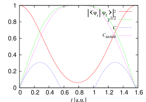
Figure 1: (Color online.) Overlap with the initial state and entanglement measures for the first two qubits, during the entanglement oscillations for five spins in a ring, generated by the Ising Hamiltonian without magnetic field in (12). In the initial state all spins are up, thus in state $\mathinner{|{0}\rangle}$ if we consider qubits. The plotted quantities are dimensionless.

In the figure we observe that the concurrence of assistance of the qubit pair is almost equal to the square root of one-tangle of one of the constituent spins. We will show later in this paper that the square root of one tangle is an upper bound for concurrence of assistance. Thus for the states in argument, the entanglement of a subsystem with the rest of the system can be indeed “focused” to a pair of qubits via suitably chosen measurement on the rest of the system. This is obvious for the cluster states, but it appears to hold for the most of the time evolution.

The dynamical entanglement behavior of the systems in argument can be controlled by the appropriate choice of the initial state. Consider for instance the following polarized initial state:

$$\left|\Psi_{\text{A}}(t=0)\right>=\mathop{\otimes}\limits_{k=1}^{N}\left(\cos\left(\frac{\theta}{2}\right)\mathinner{|{0}\rangle}_{k}+\sin\left(\frac{\theta}{2}\right)\mathinner{|{1}\rangle}_{k}\right).$$ (20)

The “A”index reflects that all the spins are rotated from the $z$ direction in the same way. This state can be prepared by a simultaneous one-qubit rotation, which is available even in optical lattice systems. If $\theta=l\pi$ ($l$ being integer), we obtain the graph state periodically, while for $\theta=l\pi/2$ the state is stationary, thus no entanglement will be generated. Between these values, the entanglement measured by one-tangle or concurrence of assistance is a monotonous and continuous function of $\theta$ for all values of time. Thus by varying this parameter of the initial state, one can control the amount of the generated entanglement.

From the above discussion we find that Ising dynamics without magnetic field has the following properties from the point of view of entanglement generation:

1. The generated bipartite entanglement is always small.

2. In the case of the cluster states one can project the state with certainty to a maximally entangled pair of two spins by a measurement on the others. Moreover, required measurement is a local one.

3. All the states of the computational basis are periodically transferred into states which have properties 1-2.

4. One can control the amount of the dynamically generated entanglement by a parameter of the initial state, which can be altered by the same local rotation applied on all the spins.

During our investigations we will check which of these properties may arise under different couplings, initial states and topologies.

IV Two properties of concurrence of assistance

In this Section we present two properties of concurrence of assistance for multi-qubit systems.

Our first proposition formulates an upper bound of concurrence of assistance.

Proposition 1

For an arbitrary state of two qubits $A$ and $B$, square root of the one-tangle of either qubits serves as an upper bound for concurrence of assistance, i.e.:

$$\sqrt{T_{A}}\geq C^{\text{assist}}_{AB}.$$ (21)

Proof: Consider the ensemble realization of the state $\varrho_{AB}$ of the qubits A,B

$$\varrho_{AB}=\sum_{k}p_{k}\mathinner{|{\xi_{k}}\rangle}\mathinner{\langle{\xi_{k}}|}$$ (22)

which provides the maximum in Eq. (10), and use the notation

$$\varrho_{k}=\mathop{\mbox{tr}}\nolimits_{B}\mathinner{|{\xi_{k}}\rangle}\mathinner{\langle{\xi_{k}}|},$$ (23)

thus

$$\varrho_{A}=\mathop{\mbox{tr}}\nolimits_{B}\varrho_{AB}=\sum_{k}p_{k}\varrho_{k},$$ (24)

due to the linearity of the partial trace. Substituting Eq. (24) into the definition in Eq. (1) we obtain

$$\sqrt{T_{A}}=2\sqrt{\det\left(\sum_{k}p_{k}\varrho_{k}\right)},$$ (25)

while according to the definition in Eq. (10),

$$C^{\text{assist}}_{AB}=2\sum_{k}\sqrt{\det(p_{k}\rho_{k})},$$ (26)

where we have exploited the fact that for pure states

$$C(\mathinner{|{\xi_{k}}\rangle})=2\sqrt{\det\varrho_{k}}.$$ (27)

Substituting Eqs. (25) and  (26) into the statement of the Proposition in inequality (21), what we have to show is that

$$\sum_{k}\sqrt{\det(p_{k}\varrho_{k})}\leq\sqrt{\det\left(\sum_{k}p_{k}\varrho_{k}\right)}.$$ (28)

This is a consequence of the recursive application of the inequality (41), which is proven in Appendix A. QED.

Intuitively, in the spirit of the considerations concerning lower bound of localizable entanglement in Ref. Popp et al. (2004), we can claim that a local measurement on the ancillary systems of a purification of $\varrho_{AB}$ cannot create additional entanglement between the spin $A$ and the rest of the system $\bar{A}$, as such a measurement is an operation on the complementary system. Thus, by choosing the optimal measurement we can, at best, concentrate all of the originally available entanglement ($\sqrt{T_{A}}$) into the entanglement between the qubits $A$ and $B$.

The appearance of the one-tangle in the context of concurrence of assistance suggests that there might be some relation with the CKW inequalities, and this is the case indeed. Nevertheless, it is simple to prove the following:

Proposition 2

For a system of three qubits $A$,$B$,$C$ in a pure state,

$$C_{AB}=C^{\text{assist}}_{AB}\ {\mathrm{and}}\ C_{AC}=C^{\text{assist}}_{AC}$$ (29)

implies that the Coffmann-Kundu-Wootters inequalities in Eq. (8) are saturated, thus

$$C_{AB}^{2}+C_{AC}^{2}=T_{A}$$ (30)

holds

This immediately follows from the same derivation as in Ref. Coffman et al. (2000) by exploiting the fact that the matrices $R_{2}$ of Eq. (5) for subsystems $AB$ and $AC$ have rank one due to the conditions of the proposition. (C.f. Eqs. (6) and (11)).

Proposition 2 relates the direct and measurement assisted approach to bipartite entanglement in multipartite systems. The question remains open, of course, whether it is true for more parties, too.

As already pointed out in Section III, for the graph states themselves $\sqrt{T_{A}}=C^{\text{assist}}_{AB}=1$, and besides $\sqrt{T_{A}}\approx C^{\text{assist}}_{AB}$ holds throughout the whole time evolution generated by Ising couplings. According to Proposition 1 it is correct to call such states as those with maximal concurrence of assistance. Meanwhile $C_{AB}\ll C^{\text{assist}}_{AB}$, which suggests that CKW inequalities are far from being saturated, which is indeed the case. The generated entanglement is essentially multipartite, but it can be converted to bipartite via a measurement. On the other hand, if CKW inequalities are saturated, then we can expect concurrence of assistance being below the square-root of one-tangle. Besides, the question naturally arises, whether it is possible to dynamically create entanglement oscillations in spin systems which saturate CKW inequalities instead.

V Controlled generation of concurrence and concurrence of assistance

Now we turn our attention to spin-1/2 systems as those naturally realize multi-qubit systems. We assign the $\hat{\sigma}^{(z)}$ eigenstates as the computational basis states as $\mathinner{|{0}\rangle}=\mathinner{|{\uparrow}\rangle}$, $\mathinner{|{1}\rangle}=\mathinner{|{\downarrow}\rangle}$. We will use the qubit notation for simplicity.

We have seen in Section III that certain states with maximal concurrence of assistance can be generated in dynamical oscillations, and the control over the available entanglement is realized by the altering of the initial state. This control requires a simultaneous operation on all the spins, and as for bipartite entanglement, it effects the entanglement available via assistive measurements only, as concurrence itself takes low values throughout the evolution. First we consider whether it is possible to control the concurrence itself too, and if it is possible to control the evolution by varying a single spin only.

Consider first a system of $N+1$ spins with XY couplings:

$$\hat{H}_{XY}=-\sum\limits_{<i,j>}\hat{\sigma}^{(x)}_{i}\hat{\sigma}^{(x)}_{j}+\hat{\sigma}^{(y)}_{i}\hat{\sigma}^{(y)}_{j},$$ (31)

in a star topology: spin $0$ is the middle one, while spins $1$ to $N$ are the outer ones, each coupled to the central one. Even though the summands of the Hamiltonian do not commute, the eigenvalues and eigenvectors can be calculated. One would expect that the state of the middle spin can control the entanglement behavior, as the interaction of the outer spins is mediated by this one. Indeed, if one considers the initial state where only the middle spin is rotated, the others point upwards, i.e. they are in the state $\mathinner{|{0}\rangle}$:

$$\left|\Psi_{\text{M}}(t=0)\right>=\left(\cos\left(\frac{\theta}{2}\right)\mathinner{|{0}\rangle}_{0}+\sin\left(\frac{\theta}{2}\right)\mathinner{|{1}\rangle}_{0}\right)\otimes\mathop{\otimes}\limits_{k=1}^{N}\mathinner{|{0}\rangle}_{k},$$ (32)

the time evolution, as shown in Appendix B, reads

$$\left|\Psi_{\text{M}}(t)\right>= \cos\left(\frac{\theta}{2}\right) \left(\mathinner{|{0}\rangle}_{0}\otimes\mathop{\otimes}\limits_{k=1}^{N}\mathinner{|{0}\rangle}_{k}\right)$$

$$+ \sin\left(\frac{\theta}{2}\right) \left(\cos(2\sqrt{N}t)\mathinner{|{1}\rangle}_{0}\otimes\mathop{\otimes}\limits_{k=1}^{N}\mathinner{|{0}\rangle}_{k}-i\sin(2\sqrt{N}t)\mathinner{|{0}\rangle}_{0}\otimes\frac{1}{\sqrt{N}}\sum\limits_{l=1}^{N}\mathinner{|{0,\ldots 0,1_{l},0\ldots}\rangle}\right).$$ (33)

The rotation of the central spin indeed controls the entanglement behavior of the system: for $\theta=0$ no entanglement is created, while for $\theta=\pi$ the maximal entanglement oscillation will appear. The state is a superposition of a product and an entangled state depending on $\theta$, thus this parameter controls the available entanglement continuously.

These entanglement oscillations are different than those in case of Ising couplings. As shown in Appendix C, concurrence is equal to concurrence of assistance in the case of any superposition of the computational basis states with all spins up and one down. This means that in the states arising throughout this evolution measurements do not facilitate “focusing” entanglement onto two spins. Besides, it has been proven in Ref. Coffman et al. (2000) that these states saturate CKW inequalities in Eq. (8), thus the bipartite entanglement present in the states is maximal. This scheme provides a dynamical way of preparing multipartite states with maximal bipartite entanglement, which is controlled by the initial state of one spin. In addition, it illustrates that Proposition 2 works for more than two subsystems, which is shown exactly in this specific case. Note that at certain times the central spin gets disentangled from the outer ring, which is meanwhile in a state with highest pairwise concurrence possible. Such a maximally entangled state is reached for the whole system, too, at different times, see also in Fig. 2/a).

In Fig. 2 we present the behavior of concurrence and square root of one tangles for a ring topology, and for an outer spin in a state different from the others, as an illustration. Here we consider the initial state producing the maximal entanglement, that is, one spin is considered to point downwards, while all the others point upwards. An analytical solution similar to that in Appendix B would be feasible too, but more energy eigenstates have nonzero weights in the initial state. Of course the functions are not equal for all the spins in such case, but their behavior is similar to the star topology. According to Appendix C, concurrence is equal to concurrence of assistance, and of course CKW inequalities are saturated.

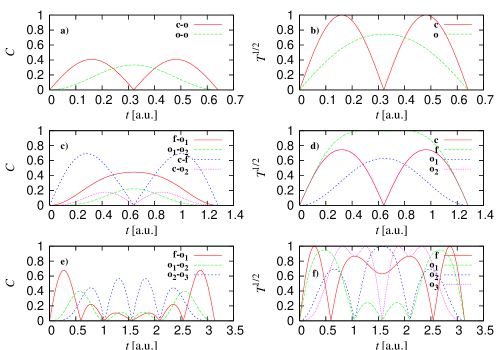
Figure 2: (Color online.) Concurrence and one-tangle for spins coupled by XY interactions in the absence of magnetic field. In Figs. a)-d) 6+1 spins are ordered into a star topology, while in e)-f) a ring of 6 spins is considered. In the initial state all spins are up, except for one, which is down. In a)-b) the central spin while in c)-d) an outer spin is flipped to point upwards. Figures on the left display concurrences of qubit pairs, those on the right display square roots of one-tangles as a function of time. Legend: c: the central central spin, f: an outer spin which is flipped initially, o_k: an outer spin which is the $k$-th neighbor of the initially flipped one. Time is measured in arbitrary units, the other quantities are dimensionless. The figure is obtained from exact numerical diagonalization and direct calculations.

From the above discussion one might conclude that the XY couplings “prefer” to generate pure bipartite entanglement. This is however not the case. In order to examine this issue, we have plotted the behavior of entanglement quantities for an XY-coupled star configuration with the initial state in Eq. (20), that is, the polarized state arising as a product of all the spins in the same state which is a superposition of $\mathinner{|{0}\rangle}$ and $\mathinner{|{1}\rangle}$. It appears that in this case concurrence between two outer spins is heavily suppressed, but concurrence of assistance takes rather high values for certain initial states. Moreover, concurrence of assistance is very close to the square-root of one-tangle, just as in the case of the Ising couplings. Thus XY couplings can, if the initial state is suitably chosen, produce states with a high amount of bipartite entanglement available via assistive measurements. Notice however, that the square-root of one-tangle is higher than concurrence of assistance, thus there is also some multipartite entanglement present in the system which cannot be accessed by assistive measurements.

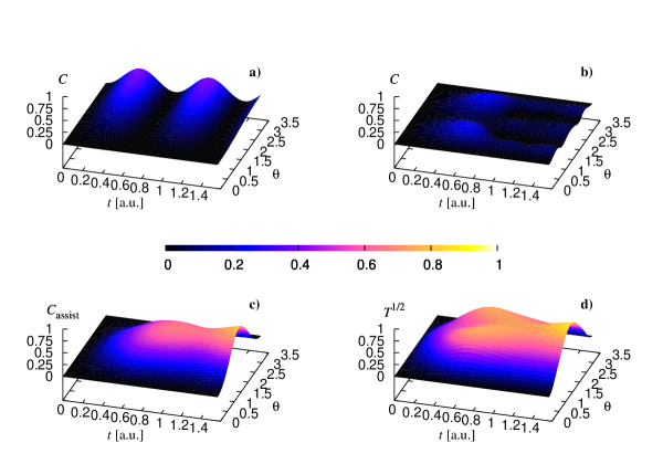
Figure 3: (Color online.) Comparison of rotating all spins or the central spin in the initial state of a 6+1 spin star with XY couplings. Fig. a) displays the temporal behavior of concurrence if the central spin is rotated, i.e. the initial state in Eq. (32) is used, while the other three figures display the evolution of concurrence, concurrence of assistance and square-root of one-tangle with an initial state in Eq. (20), that is, all spins in the same superposition of $\mathinner{|{0}\rangle}$ and $\mathinner{|{1}\rangle}$. All the bipartite quantities correspond to two outer spins, square-root of one-tangle is that of one of these. $\theta$ stands for the dimensionless parameter of the input state.

Consider now Ising interactions, and ask whether it is sufficient to rotate just one spin in order to control the amount of available entanglement, e.g. disable entanglement oscillations. For the rotation of an outer spin in the star configuration or the ring topology we have found that entanglement cannot be completely suppressed. However, if we rotate the central spin in a star topology, it is possible to control entanglement behavior. This is illustrated in Fig. 4. Similarly to the case of initial state of (20), concurrence of assistance is almost equal to the square root of one-tangle, while concurrence itself is close to zero.

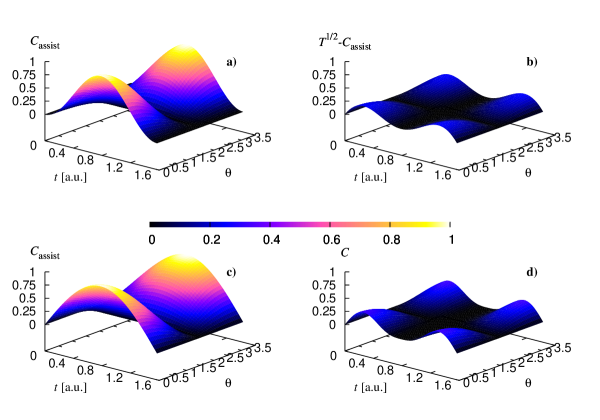
Figure 4: (Color online.) Control of entanglement generation in a system of 6+1 Ising-coupled spins in a star configuration. The central spin is rotated, i.e. initial state is that in Eq. (32), the others are in the state $\mathinner{|{0}\rangle}$. Figures a) and c) display temporal behavior of concurrence as a function of parameter $\theta$ of the initial state, for a) two outer spins and b) an outer and a central spin. Figure b) shows the difference between square root of one tangle and concurrence of assistance for two outer spins. Figure d) shows concurrence for the central and an outer spin. This quantity is zero for the outer spins.

It is important to note that the possible high value of concurrence of assistance appears to have nothing to do with the bipartite nature of the couplings. In order to see this, consider a ring of spins with the “weird” threepartite couplings

$$\hat{H}_{\text{weird}}=-\sum_{k}\hat{\sigma}^{(x)}_{k-1}\hat{\sigma}^{(y)}_{k}\hat{\sigma}^{(x)}_{k+1}.$$ (34)

The temporal behavior of concurrence of assistance and square-root of one-tangle for neighbors is shown in Fig. 5. Concurrence of assistance apparently reaches its upper limit showing that threepartite interaction can also generate maximal focusable bipartite entanglement.

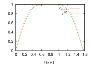
Figure 5: (Color online.) Time evolution of concurrence of assistance and one-tangle for the “weird” Hamiltonian in Eq. (34), for 6 spins. In the initial product state all spins point upwards.

In this Section we have shown that it is possible to generate entanglement oscillations not only between product and graph (or cluster) states, but also between product states, and states with maximal possible bipartite entanglement, and control this entanglement behavior by the initial state.

VI Entangled bases in the presence of a magnetic field

In Section III we have seen that in the absence of magnetic field the Ising couplings induce such dynamics that all the states of the computational basis evolve into graph states periodically. In the Heisenberg picture we may interpret this so that the product of the $\hat{\sigma}^{(z)}$ operators evolves to such a joint observable, which has an eigenbasis formed fully by graph states. One of the key features of such states is that they can be projected onto a maximally entangled state of any pair of selected spins by a von Neumann measurement on the rest of the spins. We show here that this property is preserved, moreover enhanced if the magnetic field is present.

First we consider the Ising Hamiltonian with a magnetic field pointing towards a direction characterized by the angle $\phi$:

$$\hat{H}_{\text{Ising}}=-\sum\limits_{\langle k,l\rangle}\hat{\sigma}^{(x)}_{k}\otimes\hat{\sigma}^{(x)}_{l}-B\sum_{k}e^{i\frac{\phi}{2}\hat{\sigma}^{(x)}_{k}}\hat{\sigma}^{(z)}_{k}e^{-i\frac{\phi}{2}\hat{\sigma}^{(x)}_{k}}.$$ (35)

Thus we have two free parameters characterizing the magnetic field, its magnitude $B$ and direction $\phi$. Note that the rotation of the magnetic field is equivalent to a rotation of the initial state in this case.

In particular, we are interested in the temporal behavior of the concurrence of assistance $C_{\text{assist}}$ for certain pairs of spins. Therefore we calculate the time evolution of all the states $\mathinner{|{e_{i}}\rangle}$ of the computational basis:

$$\left|e_{i}^{\prime}(B,t)\right>=\exp\left(-i\hat{H}_{\text{Ising}}t\right)\left|e_{i}\right>,\quad i=1\ldots 2^{N},$$ (36)

Then we can evaluate the average

$${\overline{C_{\text{assist}}}}(B,t)=\frac{1}{2^{N}}\sum_{i}C_{\text{assist}}\left(\left|e_{i}^{\prime}(B,t)\right>\right),$$ (37)

and also the standard deviation

$$\sigma_{C_{\text{assist}}}(B,t)=\sqrt{\overline{C_{\text{assist}}^{2}}-\overline{C_{\text{assist}}}^{2}}$$ (38)

of concurrence of assistance over the computational basis states as initial states. The deviation is informative regarding the deviation of the quantity from the average for the different initial states.

A typical result of the calculation is plotted in Fig. 6

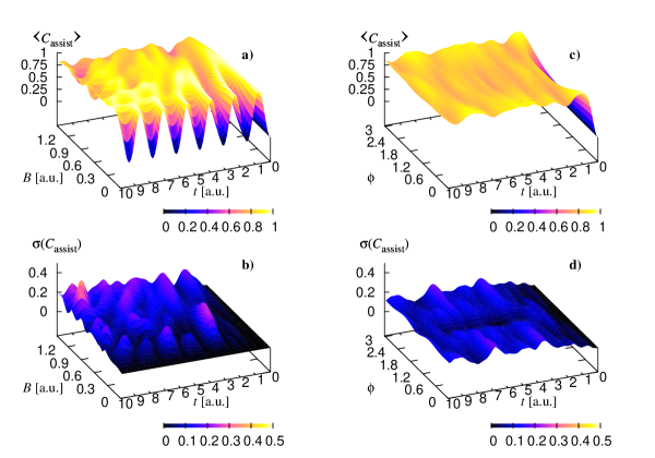
Figure 6: (Color online.) Average (a,c) and standard deviation (b,d) of concurrence of assistance for a pair of outer spins of a star topology, taken over all the possible computational basis states as initial states. Ising Hamiltonian with a magnetic field as in Eq. (35), 4+1 spins in a ring topology. In Figs. a) and b), $\phi=0$, $B$ dependence is plotted in Figs. c) and d), $B=1$, $\phi$-dependence is plotted. Similar figures are obtained for different choice of the spin pair, and ring topologies too.

For $B=0$ the expected entanglement oscillations are present. If the magnetic field is nonzero, the system does not tend to return to the initial product states. Magnetic field resolves many of the the high degeneracies of the Ising Hamiltonian, and the eigenvalues become incommensurable. Therefore, even though the evolution of the system will be almost periodic according to the quantum recurrence theorem Bocchieri and Loinger (1957), the reasonable approximate recurrences occur after an extremely long time.

For $B\neq 0$, the ensemble average of concurrence of assistance appears to be rather strictly close to one for quite long time intervals, while its standard deviation is low. The deviation can be further suppressed by the suitable choice of magnetic field. This behavior of concurrence of assistance is very similar to that in Fig. 6 also for different chosen pair of qubits, for qubit pairs of a ring topology, and also for different computationally feasible number of qubits. From this we can conclude that the elements of the computational basis are transformed into states which can be projected into nearly maximally entangled states of chosen two spins via a von Neumann measurement on the rest of the spins. Otherwise speaking, Ising couplings do take the products of $\hat{\sigma}^{(z)}$ matrices to such complete set of commuting operators, whose eigenstates have the above mentioned property. The temporal duration of the presence of this property is significantly enhanced by the magnetic field.

The so arising entanglement is essentially multipartite: the appearance of the magnetic field does not enhance concurrence of the qubit pairs as it can be verified by performing the same calculation with concurrence. Note that the characteristic behavior of the entanglement as reflected by the Meyer-Wallach measure for the kicked Ising model, also in the case of the presence of a magnetic field pointing towards an arbitrary direction was also reported in Lakshminarayan and Subrahmanyam (2004).

Another relevant question might be whether the required measurements are local, i.e. how much localizable entanglement is present. To illustrate this issue in our numerical framework, we have evaluated a lower bound for localizable entanglement by the mere consideration of a measurement on the computational basis. According to our experience, the behavior of the so available bipartite entanglement resembles that of concurrence of assistance, but takes lower values. However, quite remarkable bipartite entanglement is still available, which is in most of the cases still higher than the limit that CKW inequalities would allow for, without measurements.

Next we investigate the properties of the $XY$-model from the same point of view: into Eq. (36) we substitute the Hamiltonian

$$\hat{H}_{\text{XY}}=-\sum\limits_{\langle k,l\rangle}\left(\hat{\sigma}^{(x)}_{k}\otimes\hat{\sigma}^{(x)}_{l}+\hat{\sigma}^{(y)}_{k}\otimes\hat{\sigma}^{(y)}_{l}\right)$$

$$-\sum_{k}e^{i\frac{\phi}{2}\hat{\sigma}^{(x)}_{k}}\hat{\sigma}^{(z)}_{k}e^{-i\frac{\phi}{2}\hat{\sigma}^{(x)}_{k}}.$$ (39)

A homogeneous magnetic field parallel to the $z$ does not have any effect on the entanglement behavior of the system, as

$$\left[\sum_{l}\hat{\sigma}^{(z)};\sum\limits_{\langle k,l\rangle}\left(\hat{\sigma}^{(x)}_{k}\otimes\hat{\sigma}^{(x)}_{l}+\hat{\sigma}^{(y)}_{k}\otimes\hat{\sigma}^{(y)}_{l}\right)\right]=0$$ (40)

thus the local rotations generated by $\sum_{l}\hat{\sigma}^{(z)}$ can be taken into account after calculating the effect of the couplings. Therefore we pick $B=1$, and investigate the dependence of concurrence and concurrence of assistance on the direction $\phi$ of the field.

The quantities evaluated are again those in Eqs. (37) and (38), both for concurrence and concurrence of assistance. A typical result is displayed in Fig. 7.

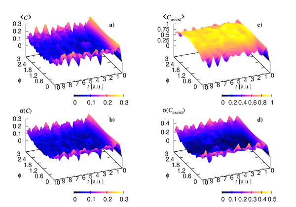
Figure 7: (Color online.) Time evolution of averages (a,c) and deviations (b,d) of concurrence (a,b) and concurrence of assistance (c,d) for two outer spins of a star configuration of 4+1 spins coupled by the XY Hamiltonian with magnetic field in (VI). Parameter $\phi$ describes the direction of the magnetic field. Similar behavior was observed for ring topologies and different choice of the qubit pair too.

It appears that for $\phi=0$ we obtain oscillations in the average concurrence, too, while concurrence of assistance is not significantly higher than concurrence itself. The appropriate choice of the direction of the magnetic field can suppress concurrence, significantly enhance concurrence of assistance and decrease its deviation. Thus even though the couplings are not Ising type, at least the feature of the Ising couplings that it produces bases with high concurrence of assistance can be retained.

VII Conclusions

In this paper we have related the problems of maximizing pairwise concurrence and pairwise concurrence of assistance in a system of multiple qubits. We have shown that the square root of one tangle of a qubit is an upper bound for the concurrence of assistance of a qubit pair containing the particular qubit. We have also shown that for a certain set of states for which the CKW inequality is known to be saturated, the concurrence is equal to the concurrence of assistance. This means that the bipartite subsystem under consideration is not correlated with the rest of the system via intrinsic multipartite entanglement.

We have also studied the entanglement behavior of spin-1/2 systems modeling qubits, from this perspective. We have shown that in a star configuration of an XY coupled spins entanglement oscillations between product states and states with maximal bipartite entanglement according to CKW inequalities can be dynamically generated. The oscillations can be controlled by rotating the spin which mediates the interaction, and at some points it gets disentangled from the rest of the outer ring, which is maximally entangled in the CKW sense. This maximal entanglement is reached for the whole system, too. We have shown numerically that the star topology facilitates the similar control of entanglement oscillations between product and graph states. The rotation of all the qubits of the initial state on the other hand leads to different behavior of concurrence of assistance, as the enhancement of bipartite entanglement to the measurement appears. We have found similar behavior for different topologies numerically.

According to our numerical results magnetic field can lead to the temporal enhancement of concurrence of assistance in the entanglement oscillations starting from the states of the computational basis, in the case of spins coupled by Ising interactions, arranged into ring or star topologies. Thereby a special entangled basis can be accessed. We have found similar behavior for the case of XY couplings: magnetic field applied along properly chosen direction suppresses concurrence and enhances concurrence of assistance.

According to the presented results, pairwise couplings between spins and qubits can be used effectively for different tasks of distributing bipartite entanglement between multiple parties. It is also possible to control the dynamical behavior of entanglement by local quantum operations such as rotation of control qubits. Besides, magnetic field can be utilized to temporally enhance certain entanglement features, or to chose between qualitatively different kinds of entanglement behavior. It would be also interesting to investigate whether the entangled bases available in the described means are useful for quantum information processing tasks.

Appendix A An inequality

In this Appendix we show, that for two Hermitian, positive semidefinite $2\times 2$ matrices $\hat{A}$ and $\hat{B}$,

$$\sqrt{\det\hat{A}}+\sqrt{\det\hat{B}}\leq\sqrt{\det\left(\hat{A}+\hat{B}\right)}$$ (41)

holds.

First we remark that for the square root of a Hermitian positive semidefinite matrix

$$\det\sqrt{\hat{A}}=\sqrt{\det\hat{A}}.$$ (42)

Thus we can rewrite inequality (41) as

$$\det\sqrt{\hat{A}}+\det\sqrt{\hat{B}}\leq\sqrt{\det\left(\hat{A}+\hat{B}\right)},$$ (43)

or equivalently,

$$\left(\det\sqrt{\hat{A}}+\det\sqrt{\hat{B}}\right)^{2}\leq\det\left(\hat{A}+\hat{B}\right).$$ (44)

Without the loss of generality we can perform calculations on the eigenbasis of $\hat{A}$. Thus we can introduce the notation

$$\sqrt{\hat{A}}=a\begin{pmatrix}a_{1}&0\cr 0&1-a_{1}\end{pmatrix}$$

$$\sqrt{\hat{B}}=b\begin{pmatrix}b_{1}&b_{2}\cr b_{2}^{*}&1-b_{1}\end{pmatrix},$$ (45)

where $a$, $b$, $a_{1}$ and $b_{1}$ are real. Substituting Eq. (45) into Eq. (44), after some calculation we obtain

$$\det\left(\hat{A}+\hat{B}\right)-\left(\det\sqrt{\hat{A}}-\det\sqrt{\hat{B}}\right)^{2}$$

$$=a^{2}b^{2}\left(|b_{2}|^{2}+(a_{1}-b_{1})^{2}\right)\geq 0,$$ (46)

which is always justified.

Note that the inequality just proven is a special property of $2\times 2$ matrices: if we replaced $\hat{A}$ and $\hat{B}$ by positive numbers as “‘$1\times 1$” matrices, the direction of inequality (41) would be reverse.

Appendix B Analytical solution for the $XY$-coupled star

Here we derive the time evolution for our specific input states in an XY coupled star configuration, based on Refs.  Hutton and Bose (2004); Breuer et al. (2004). Consider the Hamiltonian in Eq. (31) for a star topology of $N+1$ spins. Let spin 0 be the central one, thus the Hamiltonian reads

$$\hat{H}_{XY}=-\hat{\sigma}^{(x)}_{0}\sum_{k=1}^{N}\hat{\sigma}^{(x)}_{k}-\hat{\sigma}^{(y)}_{0}\sum_{k=1}^{N}\hat{\sigma}^{(y)}_{k}.$$ (47)

Introducing the joint spin operators of the outer spins

$$\hat{J}_{\alpha}=\sum_{k=1}^{N}\frac{1}{2}\hat{\sigma}_{\alpha},\qquad\alpha=x,y,z,$$

$$\hat{J}_{\pm}=\sum_{k=1}^{N}\hat{J}_{x}\pm i\hat{J}_{y}$$ (48)

and the operator for the $z$ component of the total angular momentum

$$\hat{L}_{z}=\hat{J}_{z}+\frac{1}{2}\hat{\sigma}^{(z)},$$ (49)

the following commutation relations hold:

$$\left[\hat{H}_{XY},\hat{L}_{z}\right]=\left[\hat{H}_{XY},\hat{J}^{2}\right]=0.$$ (50)

Therefore the computational basis states with equal spins down span invariant subspaces of the evolution, and the outer spins behave collectively as one big spin. It is convenient to rewrite the Hamiltonian in the Jaynes-Cummings type form

$$\hat{H}_{XY}=-\left(\hat{\sigma}^{(+)}_{0}\hat{J}_{-}+\hat{\sigma}^{(-)}_{0}\hat{J}_{+},\right)$$ (51)

which has the eigenvalues and eigenvectors

$$\mathinner{|{\phi_{j,m,\pm}}\rangle}=\frac{1}{\sqrt{2}}\left(\mathinner{|{1}\rangle}\mathinner{|{j;m}\rangle}\pm\mathinner{|{0}\rangle}\mathinner{|{j;m-1}\rangle}\right)$$

$$\omega_{j,m,\pm}=\mp 2\sqrt{(j+m)(j-m+1)},$$ (52)

where the states $\mathinner{|{j;m}\rangle}$ are the eigenvectors for the outer spins, while the states $\mathinner{|{0}\rangle}$ and $\mathinner{|{1}\rangle}$ are the states of the central spin in our qubit notation. (Note that in our notation, $\mathinner{|{0}\rangle}=\mathinner{|{\uparrow}\rangle}$, thus $\hat{\sigma}^{(+)}\mathinner{|{1}\rangle}=2\mathinner{|{0}\rangle}$.)

We consider the possibility of the control by the rotation of the central spin, thus our initial state reads

$$\left|\Psi(t=0)\right>=A_{0}\left|0\right>\otimes\left|00\ldots\right>+A_{1}\left|1\right>\otimes\left|00\ldots\right>=A_{0}\left|0\right>\otimes\left|j=\frac{N}{2},m=\frac{N}{2}\right>+A_{1}\left|1\right>\otimes\left|j=\frac{N}{2},m=\frac{N}{2}\right>.$$ (53)

Rewriting this in the energy basis in Eq. (B) we obtain

$$\left|\Psi(t=0)\right>=A_{0}\left|0\right>\otimes\left|j=\frac{N}{2},m=\frac{N}{2}\right>+\frac{A_{1}}{2}\left(\left|1\right>\otimes\left|j=\frac{N}{2},m=\frac{N}{2}\right>+\left|1\right>\otimes\left|j=\frac{N}{2},m=\frac{N}{2}-1\right>\right)$$

$$+\frac{A_{1}}{2}\left(\left|1\right>\otimes\left|j=\frac{N}{2},m=\frac{N}{2}\right>-\left|1\right>\otimes\left|j=\frac{N}{2},m=\frac{N}{2}-1\right>\right).$$ (54)

Substituting the $e^{-i\omega t}$ factors, where according to Eq. (B), the $\omega$-s are $0,-2\sqrt{N},+2\sqrt{N}$ for the three summands of Eq. (B) respectively, after some algebra we obtain

$$\left|\Psi(t=0)\right>=A_{0}\left|0\right>\otimes\left|0,0,\ldots\right>+A_{1}\left(\cos(2\sqrt{N}t)\mathinner{|{1}\rangle}\otimes\mathinner{|{0,0,\ldots}\rangle}-i\sin(2\sqrt{N}t)\mathinner{|{0}\rangle}\otimes\left|j=\frac{N}{2},m=\frac{N}{2}-1\right>\right).$$ (55)

This shows that the complex phases of $A_{0}$ and $A_{1}$ are irrelevant from the point of view of the entanglement properties. Substituting $A_{0}=\cos(\theta/2)$ and $A_{1}=\sin(\theta/2)$ into Eq. (55), and calculating $\mathinner{|{j=N/2,m=N/2-1}\rangle}$ by applying $\hat{J}_{-}$ on $\mathinner{|{j=N/2,m=N/2}\rangle}$, we obtain Eq. (V), the desired result.

Appendix C Relation of concurrence and concurrence of assistance for states with maximum one spin down

In this appendix we show that for states of $N$ qubits of the form

$$\left|\Psi_{1}\right>=\sum_{k=0}^{N}A_{k}\mathinner{|{\underline{k}}\rangle}$$ (56)

where

$$\mathinner{|{\underline{0}}\rangle} = \mathinner{|{0,0,\ldots,0}\rangle},$$

$$\mathinner{|{\underline{k}}\rangle} = \mathinner{|{0,\ldots 0,1_{k},0\ldots}\rangle},\quad k\neq 0,$$ (57)

concurrence equals to concurrence of assistance for any pairs of the qubits.

Consider the spins $k$ and $l$. Their density matrix in the computational basis is of the form

$$\varrho^{(kl)}=\begin{pmatrix}\varrho_{00,00}&\varrho_{00,01}&\varrho_{00,10}&0\cr\varrho_{00,01}^{*}&\varrho_{01,01}&\varrho_{01,10}&0\cr\varrho_{00,10}^{*}&\varrho_{01,10}^{*}&\varrho_{10,10}&0\cr 0&0&0&0\end{pmatrix}$$ (58)

Direct calculation of concurrence and concurrence of assistance according to Eqs. (6) and Eq. (11) yields

$$C_{kl}=2|\varrho_{01,10}|,\qquad C^{\text{assist}}_{kl}=2\sqrt{\varrho_{01,01}\varrho_{10,10}}.$$ (59)

Calculating the required matrix elements from Eq. (56) we find

$$\varrho_{01,01}=A_{k}^{*}A_{k},\quad\varrho_{10,10}=A_{l}^{*}A_{l},\quad\varrho_{01,10}=A_{k}^{*}A_{l}.$$ (60)

Substituting Eq. (60) into Eq. (59) gives $C_{kl}=C^{\text{assist}}_{kl}$ for arbitrary k,l.

References

- Koashi et al. (2000) M. Koashi, V. Bužek, and N. Imoto, Phys. Rev. A 62, 050302 (2000).
- Plesch and Bužek (2003) M. Plesch and V. Bužek, Phys. Rev. A 67, 012322 (2003).
- Plesch and Bužek (2002) M. Plesch and V. Bužek, Quantum Inform. Comput. 2, 530 (2002).
- Coffman et al. (2000) V. Coffman, J. Kundu, and W. K. Wootters, Phys. Rev. A 61, 052306 (2000).
- O’Connor and Wootters (2001) K. M. O’Connor and W. K. Wootters, Phys. Rev. A 63, 052302 (2001).
- Briegel and Raussendorf (2001) H. J. Briegel and R. Raussendorf, Phys. Rev. Lett. 86, 910 (2001).
- Hein et al. (2004) M. Hein, J. Eisert, and H. J. Briegel, Phys. Rev. A 69, 062311 (2004).
- Raussendorf and Briegel (2001) R. Raussendorf and H. J. Briegel, Phys. Rev. Lett. 86, 5188 (2001).
- Raussendorf et al. (2003) R. Raussendorf, D. E. Browne, and H. J. Briegel, Phys. Rev. A 68, 022312 (2003).
- DiVincenzo et al. (1998) D. P. DiVincenzo, C. A. Fuchs, H. Mabuchi, J. A. Smolin, A. Thapliyal, and A. Uhlmann, (Springer-Verlag, 1998), vol. 1509 of Lecture notes in computer science, e-print quant-ph/9803033.
- Laustsen et al. (2003) T. Laustsen, F. Verstraete, and S. J. Van Enk, Quantum Inform. Comput. 3, 64 (2003).
- Verstraete et al. (2004) F. Verstraete, M. Popp, and J. I. Cirac, Phys. Rev. Lett. 92, 027901 (2004).
- Popp et al. (2004) M. Popp, F. Verstraete, M. A. Martin-Delgado, and J. I. Cirac, e-print quant-ph/0411123 (2004),.
- Bose (2003) S. Bose, Phys. Rev. Lett. 91, 207901 (2003).
- Christandl et al. (2004) M. Christandl, N. Datta, A. Ekert, and A. J. Landahl, Phys. Rev. Lett. 92, 187902 (2004).
- Osborne and Nielsen (2004) T. J. Osborne and N. Nielsen, Phys. Rev. A 69, 052315 (2004).
- Schuch and Siewert (2003) N. Schuch and J. Siewert, Phys. Rev. A 67, 032301 (2003).
- Yung et al. (2004) M. H. Yung, D. W. Leung, and S. Bose, Quantum Inform. Comput. 4, 174 (2004).
- Chiara et al. (2004) G. D. Chiara, R. Fazio, C. Machiavello, S. Montagero, and G. M. Palma, Phys. Rev. A 70, 062308 (2004).
- Garcia-Ripoll and Cirac (2003) J. J. Garcia-Ripoll and J. I. Cirac, New J. Phys. 5, 76 (2003).
- Amico et al. (2004) L. Amico, A. Osterloh, F. Plastina, R. Fazio, and G. M. Palma, Phys. Rev. A 69, 022304 (2004).
- Subrahmanyam (2004) V. Subrahmanyam, Phys. Rev. A 69, 034304 (2004).
- Plastina et al. (2004) F. Plastina, L. Amico, A. Osterloh, and R. Fazio, New J. Phys. 6, 124 (2004).
- Lakshminarayan and Subrahmanyam (2004) A. Lakshminarayan and V. Subrahmanyam, e-print quant-ph/0409039 (2004).
- Subrahmanyam and Lakshminarayan (2004) V. Subrahmanyam and A. Lakshminarayan, e-print quant-ph/0409048 (2004).
- Vidal et al. (2004) J. Vidal, G. Palacios, and C. Aslangul, Phys. Rev. A 70, 062304 (2004).
- Vidal et al. (2001) G. Vidal, L. Masanes, and J. Cirac, e-print quant-ph/0102037 (2001).
- Nielsen and Chuang (1997) M. A. Nielsen and I. L. Chuang, Phys. Rev. Lett. 79, 321 (1997).
- Hillery et al. (2002a) M. Hillery, V. Bužek, and M. Ziman, Phys. Rev. A 65, 022301 (2002a).
- Hillery et al. (2002b) M. Hillery, M. Ziman, and V. Bužek, Phys. Rev. A 66, 042302 (2002b).
- Borhani and Loss (2004) M. Borhani and D. Loss, e-print quant-ph/0410145 (2004).
- Hutton and Bose (2004) A. Hutton and S. Bose, Phys. Rev. A 69, 042312 (2004).
- Breuer et al. (2004) H.-P. Breuer, D. Burgarth, and F. Petruccione, Phys. Rev. A 70, 045323 (2004).
- Hill and Wootters (1997) S. Hill and W. K. Wootters, Phys. Rev. Lett. 78, 5022 (1997).
- Wootters (1998) W. K. Wootters, Phys. Rev. Lett. 80, 2245 (1998).
- Osborne (2005) T. J. Osborne, e-print quant-ph/0502176 (2005).
- Bocchieri and Loinger (1957) P. Bocchieri and A. Loinger, Phys. Rev. 107, 337 (1957).