Entanglement manipulation by a local magnetic pulse

Abstract

A scheme for controlling the entanglement of a two-qubit system by a local magnetic pulse is proposed. We show that the entanglement of the two-qubit system can be increased by sacrificing the coherence in ancillary degree of freedom, which is induced by a local manipulation.

Quantum entanglement plays a central role in quantum information and quantum computation Nielsen1 ; AGalindo02 . It is in the heart of most quantum phenomena, such as quantum teleportation, dense coding, and quantum cryptography Bennett . Thus, the issue of creating two-particle entanglement in various composite systems is of great importance in technology development. For example, in nuclear magnetic resonance experiments (NMR)LMKVandersypen04 ; ILChuang98 ; SLloyd98 ; RJNelson00 , significant efforts were put in creating Bell states and Greenberger- Horne-Zeilinger (GHZ) state. Schemes for producing entangled state using adiabatic population transfer based on a two-spin system have also been proposedRGUnanyan01 ; BZhou04 . Quite recently, it has been shown that the existence of relative phase between two Rabi frequencies can be used to control entanglement of the two-qubit system at willVSMalinovsky04 .

As it is well known, the entanglement is intrinsically related to the superposition principle of quantum mechanics. Thus the problem of creating or controlling the entanglement is simply the problem of coherent control of population transfer between different levels of a composite system. For example, the maximally entangled state $(|00\rangle+|11\rangle)/\sqrt{2}$ can be created from a fully polarized state $|00\rangle$ by transferring half of its population to state $|11\rangle$ through a careful controlled adiabatic process: $|00\rangle\rightarrow|01\rangle\rightarrow|11\rangle$. A successful realization of population transfer depends on the adiabatic condition and can be achieved through a careful control of pulse shape with an appropriate choice of the Rabi oscillation frequencyPMarte91 ; MWeitz94 .

On the other hand, in order to be useable for quantum information process, one particle of the prepared entangled state has to be sent through a classical channel. Then the entanglement between the two particles, in general, will be weakened because of its interference with the environment. However, in some purposes such as teleportation, the entanglement must be supplied in the form of maximally entangled pairs. Therefore the entanglement distillationBennett1 is of importance in quantum information. Through a method called Schmidt projection, it has been shown that the entanglement of $n$ partly entangled states can be concentrated into a small number of maximally entangled pairsCHBennett96 .

In this paper, we propose a method to control the entanglement of two separated systems by modulating a local oscillating field which is used to create coherent superposition in one of the two systems. We show, as long as the entanglement is non-zero, the entanglement can be modulated to reach a maximum with a certain probability via an appropriate choice of tuning period and radio magnitude. Therefore, we can choose the pulse strength or the tuning period or both as the control knob to create the state with desired entanglement, especially the maximally entangled state. As we will show below, the external oscillation in our method only interacts with one of the particle and can be controlled locally. This method is different from the Schmidt projectionCHBennett96 . Therefore, the suggested method opens a new avenue for entanglement distillation and facilitates experimental implementation on quantum information transmission.

Entanglement evolution and projection: We consider two separated non-interacting particles called A and B, shared between Alice and Bob respectively. In addition to the spin degree of freedom which are partly entangled between A and B, such as the state $\cos(\theta)|\uparrow\uparrow\rangle+\sin(\theta)|\downarrow\downarrow\rangle$, the system has other ancillary degree of freedom denoted as $|0\rangle$ and $|1\rangle$. This ancillary degree of freedom might be the orbital state in spin-orbit interacting systems, energy level of quantum dot, or level of ions in magnetic trap. For convenience, we call it band hereafter. Therefore, there are four possible local states, i.e., $|0\uparrow\rangle$, $|1\uparrow\rangle$, $|0\downarrow\rangle$, and $|1\downarrow\rangle$, either for particle A or particle B. In a magnetic field, the Hamiltonian of particle A and particle B can be written as

$$H_{0}^{A(B)}=-[\omega_{s}\sigma^{z}+\omega_{b}\tau^{z}-J\sigma^{z}\tau^{z}],$$ (1)

which is typical in the NMR systemsLMKVandersypen04 . Here $\omega_{s},\omega_{b}$ are the Larmor frequency for spin ($\sigma^{z}$) and band ($\tau^{z}$) respectively, while the scalar coupling $J$ can be interpreted as the coupling from band to an additional static field along $z$ direction produced by spin (or vice versa). Clearly, the Hamiltonian is diagonal in the standard basis, and the corresponding eigenvalues are

$$\varepsilon_{1}=-\omega_{s}-\omega_{b}+J,\;\;\varepsilon_{2}=-\omega_{s}+\omega_{b}-J,$$

$$\varepsilon_{3}=\omega_{s}-\omega_{b}-J,\,\;\;\;\;\varepsilon_{4}=\omega_{s}+\omega_{b}+J.$$ (2)

Since we are interested in the entanglement between the two spins, it is assumed that the two spins in the initial state are not maximally entangled, while two bands are fully polarized. Mathematically, we assume that the initial state takes the form

$$\Psi(t=0)=\cos\theta|0\uparrow\rangle_{A}|0\uparrow\rangle_{B}+\sin\theta|0\downarrow\rangle_{A}|0\downarrow\rangle_{B}.$$ (3)

Here the partly entangled state is not restricted to the form $\cos\theta|\uparrow\uparrow\rangle+\sin\theta|\downarrow\downarrow\rangle$, it can be in other forms, such as $\cos\theta|\downarrow\uparrow\rangle-\sin\theta|\downarrow\uparrow\rangle$. The entanglement of two spins in this state, measured by the concurrenceWKWootters98 , is $C(t=0)=|\sin 2\theta|$. Thus the first problem is to find a possible magnetic pulse that leads to a unitary time evolution, and then to modulate the population of $|\uparrow\rangle_{A}|\uparrow\rangle_{B}$ and $|\downarrow\rangle_{A}|\downarrow\rangle_{B}$. For this purpose, we add an ideal rectangular transversal magnetic pulse with frequency $\omega$ on particle B. This additional Hamiltonian can be simplified as

$$H^{B}_{R}=g[e^{i\omega t+i\phi}\tau^{\dagger}+h.c.]$$ (4)

where $\tau^{+}|0\rangle_{B}=|1\rangle_{B},\,\tau^{-}|1\rangle_{B}=|0\rangle_{B}$, $\phi$ is the relative phase and $g$ is the magnitude of the magnetic pulse. Thus the whole Hamiltonian of the two-particle system is

$$H=H^{A}_{0}+H^{B}_{0}+H_{R}^{B},$$

and the time-dependent Schrödinger equation reads

$$H\Psi(t)=i\frac{i\partial}{\partial t}\Psi(t).$$ (5)

In order to eliminate the time dependence of the Hamiltonian of particle B: $H^{B}=H^{B}_{0}+H_{R}^{B}$, we apply a unitary transformation

$$U = e^{-i\omega t}|0\uparrow\rangle_{BB}\langle 0\uparrow|+e^{i\omega t}|1\uparrow\rangle_{BB}\langle 1\uparrow|$$ (6)

$$+ e^{-i\omega t}|0\downarrow\rangle_{BB}\langle 0\downarrow|+e^{i\omega t}|1\downarrow\rangle_{BB}\langle 1\downarrow|.$$

Then the effective “rotating frame” Hamiltonian matrix of particle B becomes

$$H^{B}_{U}=UH^{B}U-iU\frac{\partial}{\partial t}U^{\dagger}$$ (7)

$$=\left(\begin{array}[]{cccc}\varepsilon_{1}^{B}+\omega/2&ge^{i\phi}&0&0\\ ge^{-i\phi}&\varepsilon_{2}^{B}-\omega/2&0&0\\ 0&0&\varepsilon_{3}^{B}+\omega/2&ge^{i\phi}\\ 0&0&ge^{-i\phi}&\varepsilon_{4}^{B}-\omega/2\end{array}\right)$$ (12)

in the standard basis $|0\uparrow\rangle_{B},|1\uparrow\rangle_{B},|0\downarrow\rangle_{B},|1\downarrow\rangle_{B}$ of particle B. The eigenvalues of $H^{B}_{U}$ are

$$E_{1(2)}=\frac{1}{2}\left[(\varepsilon_{1}^{B}+\varepsilon_{2}^{B})\pm\sqrt{(\varepsilon_{1}^{B}-\varepsilon_{2}^{B}+\omega)^{2}+4g^{2}}\right]$$ (13)

$$E_{3(4)}=\frac{1}{2}\left[(\varepsilon_{3}^{B}+\varepsilon_{4}^{B})\pm\sqrt{(\varepsilon_{3}^{B}-\varepsilon_{4}^{B}+\omega)^{2}+4g^{2}}\right]$$ (14)

and the corresponding eigenvectors are

$$\psi_{1(2)}=|0\uparrow\rangle_{B}+e^{-i\phi}\left(\pm\sqrt{1+\eta_{12}^{2}}-\eta_{12}\right)|1\uparrow\rangle_{B},$$ (15)

$$\psi_{3(4)}=|0\downarrow\rangle_{B}+e^{-i\phi}\left(\pm\sqrt{1+\eta_{34}^{2}}-\eta_{34}\right)|1\downarrow\rangle_{B},$$ (16)

where $\eta_{ij}=(\varepsilon^{B}_{i}-\varepsilon^{B}_{j}+\omega)/2g$ is a dimensionless parameter. We choose $\omega=\varepsilon_{2}-\varepsilon_{1}=2\omega_{b}-2J$ and take the weak field limit, i.e., $\eta_{34}\gg 1$. Then the dynamics of the whole system is dominated by the resonance between $|0\uparrow\rangle_{B}$ and $|1\uparrow\rangle_{B}$ in system B. Therefore, to the order of $O(1/\eta_{34})$, the wave function of the two particles can be expressed as

$$\Psi(t) = c_{0}(t)|0\downarrow\rangle_{A}|0\downarrow\rangle_{B}+c_{1}(t)|0\uparrow\rangle_{A}|0\uparrow\rangle_{B}$$ (17)

$$+c_{2}(t)|0\uparrow\rangle_{A}|1\uparrow\rangle_{B},$$

with the amplitude $c_{i}(t),i=1,2,3$ as

$$c_{0}(t)=e^{-i(\varepsilon_{3}^{A}+\varepsilon_{3}^{B})t}\sin\theta,$$

$$c_{1}(t)=e^{-i(\varepsilon_{1}^{A}+\varepsilon_{1}^{B})t}\cos(gt)\cos\theta,$$ (18)

$$c_{2}(t)=e^{-i(\varepsilon_{1}^{A}+\varepsilon_{2}^{B})t}\sin(gt)\cos\theta e^{-i(\phi+\pi/2)}.$$

Therefore the magnetic pulse introduces a resonance for particle B via an appropriate choice on the frequency, and the resonance depresses the amplitude of $|0\uparrow\rangle_{A}|0\uparrow\rangle_{B}$. Obviously, the population transfer here is selective and the resonance can be regarded as a filterDYang04 in the process of population transfer. We show that the population dynamics of the corresponding frequency in Fig. 1(a) for the case of $\theta=\pi/6$. Obviously, the entanglement of the two spins is also suppressed by the local magnetic pulse, and it evolves in the form of

$$C(t)=|\sin(2\theta)\cos(gt)|=C(t=0)|\cos(gt)|$$

as time elapses. This is consistent with the fact that the local operation and classical communication can not increase the entanglement between two parties.

In order to increase the entanglement between particle A and B, we now perform a following projection measurement on particle B,

$$P_{0}=|0\rangle_{BB}\langle 0|,\;P_{1}=|1\rangle_{BB}\langle 1|.$$ (19)

After the measurement, the band of particle B will be projected onto state $|0\rangle_{B}$ and $|1\rangle_{B}$ with probability $\sin^{2}\theta+\cos^{2}\theta\cos^{2}(gt)$ and $\cos^{2}\theta\sin^{2}(gt)$, respectively. Clearly, the latter case makes no sense because the entanglement between two particles is completely destroyed. We are only interested in the former case in which the output state becomes

$$\Psi^{\prime}(t)=\frac{\left[c_{0}(t)|0\downarrow\rangle_{A}|0\downarrow\rangle_{B}+c_{1}(t)|0\uparrow\rangle_{A}|0\uparrow\rangle_{B}\right]}{\sqrt{c_{0}(t)^{2}+c_{1}(t)^{2}}}.$$ (20)

This state may possess higher entanglement than the original state, as reflected by its concurrence measure

$$C^{\prime}(t)=\frac{\sin(2\theta)\cos(gt)}{\sin^{2}\theta+\cos^{2}\theta\cos^{2}(gt)}$$ (21)

which reaches maximum $C^{\prime}=1$ at the condition $\cos(gt)=\tan\theta$, as is shown in Fig. 1(c). This properties is completely different from the behavior of $C(t)$, which is always suppressed during the evolution. The reason we have such behavior of $C^{\prime}(t)$ is due to the superposition principle of quantum mechanics. Therefore, Bob could tell Alice in a classical way whether his projection measurement is successful or not and only when the output of his measurement is $|0\rangle_{B}$, the final state is entangled, otherwise it is not entangled.

In short, we summarize the whole procedure as follows

• First, if Alice and Bob initially share a partly entangled state, such as $\cos\theta|\uparrow\rangle_{A}|\uparrow\rangle_{B}+\sin\theta|\downarrow\rangle_{A}|\downarrow\rangle_{B}$, then Bob will switch on a magnetic pulse to transfer the population of $|\uparrow\rangle_{A}|\uparrow\rangle_{B}$ to a target state which is distinguished by introducing an ancillary degree of freedom.

• Second, Bob does a projection measurement in the space of ancillary degree of freedom.

• Finally, Bob tells Alice his projection measurement result through a classical channel.

This completes the procedure for a single pair. Clearly, the third step is quite necessary since the final result depends on the probability of the projection measurement (19).

Figure 1: (a) Population dynamics of the state $|00\rangle|\downarrow\downarrow\rangle$ (solid line), $|00\rangle|\uparrow\uparrow\rangle$ (dashed line) and $|01\rangle|\uparrow\uparrow\rangle$ (dotted line) for the case of $\theta=\pi/6$. (b) The evolution of the concurrence between the two spins. (c) The evolution of the concurrence if the projection measurement is successful. Here, the time is in unit of $1/g$.

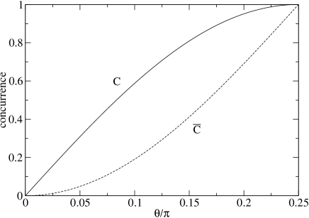
Figure 2: The original concurrence $C(t=0)$ (solid line) and final average concurrence $\bar{C}$(dashed line) as a function of $\theta/\pi$.

Efficiency: In the above, we have shown that the entanglement of a pair of the two-qubit system can be enhanced with a certain probability by creating the coherence in the ancillary degree of freedom and a follow up projection measurement on them. Now we consider a large number ($N$) of partial entangled pairs. Obviously we can only obtain a small number of maximally entangled state, such as singlets, due to its finite probability in the measurement process (19). Introducing the final average concurrence as ${\bar{C}}=N^{\prime}/N$ where $N^{\prime}$ denotes the number of pairs with maximum entanglement ($C^{\prime}=1$) after the projection measurement. Clearly ${\bar{C}}$ depends on the value of $\theta$ as was shown in Fig. 2, from which we see that although we can generate state with higher entanglement, ${\bar{C}}$ still can not exceed $C$ at any value of $\theta$. Moreover, even though the concurrence is concave function of $\theta$, ${\bar{C}}$ is not. We attribute this result to its dependence on the probability of the projection measurement rather than the initial entanglement itself. We define the efficiency as $R\equiv\frac{\bar{C}}{C}$ where $C=|\sin(2\theta)|$ is the initial concurrence. For the present case, it is calculated as $\tan(\theta),(0\leq\theta\leq\pi/4)$.

Discussion and summary: In this work, we proposed a scheme to control the entanglement between two separated systems by introducing a local magnetic pulse and a follow up projection measurement on the ancillary degree of freedom. Our scheme is quite different from the one proposed by Bennett et al, which operates the projection on the whole state of $N$ pairs, while we do it on individual pairs, so it is easier to be realized by experiment. In our scheme, the function of the rectangular magnetic pulse is to establish the coherence between the ancillary degree of freedom, i.e., to transfer partial population to a target state. Experimentally, this process can be completed by using adiabatic transfer interferometerPMarte91 ; MWeitz94 . Meanwhile, we would like to point out that the population transfer here is selective, and it is realized via a magnetic resonance. Therefore, another important feature of the magnetic pulse is that it act as a filterDYang04 . The selective population transfer or the filter can also be realized according to the Pauli exclusion principle or theory of forbidden band in quantum mechanics (For example, spin filter in condensed matter physicsPRecher00 ).

Moreover, our scheme can be easily generalized to multi-level state as well as mixed state. Take the latter as an example, if the initial state is $\rho(0)$, the problem then becomes to find a method to modulate the entry of $\rho(0)$ by introducing one or more ancillary degree of freedom and a magnetic pulse to realize the population transfer. That is, during the time evolution, the mixed state can be written as $\rho(t)=\rho_{1}(t)+\rho_{2}(t)$ where $\rho_{1}(t)$ and $\rho_{2}(t)$ are characterized by the ancillary degree of freedom and $\rho_{1}(t)$ is assumed to possess higher entanglement then $\rho(0)$. Then after a projection measurement, the state can be be projected to the desired state $\rho_{1}$ with a certain probability.

This work is supported by the Earmarked Grant for Research from the Research Grants Council (RGC) of the HKSAR, China (Project CUHK 401504). SJGU thanks D. Yang for helpful and stimulating discussions, We shank S. Y. Zhu for helpful comments and discussions.

References

- (1) M. A. Nilesen and I. L. Chuang, Quantum Computation and Quantum Information (Cambridge University Press, Cambridge, England, 2000)
- (2) A. Galindo and M. A. Martin-Delgado, Rev. Mod. Phys. 74, 347 (2002).
- (3) C. H. Bennett and S. J. Wiesner, Phys. Rev. Lett., 68, 557 (1992); C. H. Bennett, G. Brassard, C. Crepeau, R. Jozsa, A. Peres, and W. Wootters, Phys. Rev. Lett., 70, 1895 (1993).
- (4) For example, L. M. K. Vandersypen and I. L. Chuang, Rev. Mod. Phys. 76, 1037 (2004).
- (5) N. A. Gershenfeld and I. L. Chuang, Science 275, 350 (1997); I. L. Chuang, et al, Prog. R. Soc. London, Ser. A 454, 447 (1998).
- (6) S. Lloyd, Phys. Rev. A 57, R1473 (1998);
- (7) R. J. Nelson, D. G. Cory, and S. Lloyd, Phys. Rev. A 61, 022106 (2000).
- (8) R. G. Unanyan, N. V. Vitanov, and K. Bergmann, Phys. Rev. Lett. 87, 137902 (2001); R. G. Unanyan, B. W. Shore, and K. Bergmann, Phys. Rev. A 63, 043405 (2001).
- (9) B. Zhou, R. Tao, and S. Q. Shen, Phys. Rev. A 70, 022311 (2004).
- (10) V. S. Malinovsky and I. R. Sola, Phys. Rev. Lett. 93, 190502 (2004).
- (11) P. Marte, P. Zoller, and J. L. Hall, Phys. Rev. A 44, R4118 (1991).
- (12) M. Weitz, B. C. Young, and S. Chu, Phys. Rev. Lett. 73, 2563 (1994).
- (13) C. H. Bennett, D.P. DiVincenzo, J. A. Smolin and W. K. Wootters, Phys. Rev. A 54, 3824 (1996).
- (14) C. H. Bennett, H. J. Bernstein, S. Popescu, and B. Schumacher, Phys. Rev. A 53, 2046 (1996).
- (15) W. K. Wootters, Phys. Rev. Lett. 80, 2245 (1998); S. Hill and W. K. Wootters, Phys. Rev. Lett. 78, 5022 (1997).
- (16) Dong Yang, Sixia Yu, quant-ph/0410187
- (17) For example, P. Recher, E. V. Sukhorukov, and D. Loss, Phys. Rev. Lett. 85, 1962(2000).