Necessity of Combining Mutually Incompatible Perspectives in the Construction of a Global View: Quantum Probability and Signal Analysis

Abstract

The scientific fields of quantum mechanics and signal-analysis originated within different settings, aimed at different goals and started from different scientific paradigms. Yet the development of the two subjects has become increasingly intertwined. We argue that these similarities are rooted in the fact that both fields of scientific inquiry had to deal with finding a single description for a phenomenon that yields complete information about itself only when we consider mutually incompatible accounts of that phenomenon.

Keywords: quantum probability, signal analysis, incompatible observables, observation, global view.

1 Introduction

Can we find a single common framework for all knowledge that in some way converges to the truth, or should we perhaps accept that truth is inevitably only meaningful with respect to the one who pronounces it, to the context in which it is produced, to the frame of reference it is presented in? The simple question we pose here is well-known to lead to endless discussion on the nature of reality and knowledge, the relation between ontology and epistemology and between theory and fact. This discussion itself is an illustration of the dichotomic status of truth. The various stances taken by the participants in the discussion contribute to the idea of a relative truth, but the mere fact that we are still discussing the issue, highlights that we still have not given up on trying to convince each other that one truth is perhaps “more” true, than another. In the face of all various dispositions and discourses, along with the multiplicity of interpretation that is generated by these, many a thinker has given up on the idea of an absolute truth. If truth is only meaningful relative to a context or framework, we must ask: what is a context? Either one accepts the truth of a given definition of context, embracing once more the notion of an absolute truth, or one accepts that the relation between truth and context is a relative one: truth is defined by the framework that produced it, and the framework is that in which certain, given truths hold. We believe this problem of the nature of truth, and especially the popular tendency to congregate around an extreme interpretation of the idea of relative truth, has undermined the believe of rationality as a way to approach truth. Yet there are branches of human activity that embrace the absolute notion of truth, simply because in some cases, one cannot afford to succumb to relative truth. Take a court trial as an example. Despite all various and often contradictory accounts of witnesses, a judge or jury must believe that some unique set of events has happened which are to be judged as criminal or not by the court. It is an implicit but nevertheless crucial assumption that lies at the basis of our judicial system, that one single reality has given rise to all various accounts, and not that every testimony has the ability to create its own, independent reality. The exact sciences, by their very nature, were also among those that have shown great reluctance to accept the notion of relative truth. We can find a paradigmatic example of this struggle in the wave–particle duality in the description of elementary particles or quanta. Another area of research that faces similar problems, i.e. a plurality of descriptions of the same signal, is the field of signal analysis. Therefore, it may not come as a great surprise that there are certain characteristic features in the mathematical description of these two theories that display similarities. Yet both fields are usually considered only connected on a mathematical level, but to such extent that quite a few of the more important definitions in signal analysis are borrowed from earlier developments in quantum physics. We believe a very deep connection can be identified in the way these theories relate the results of observation to the state of the system which was observed. We will give brief, mildly technical introductions to both fields of study and invoke a metaphor from analytic geometry that, we believe, shows why the similarities between the two are not coincidental, but emerged from the problem of attributing truth to different, incompatible perspectives of the same phenomenon. Finally we argue for the relevance and even necessity of combining mutually incompatible perspectives in other fields of knowledge.

2 The birth of quantum mechanics

In 1925 a radically new theory of the fundamental constituents of matter and energy was born. The final form the theory was to take, emerged from two different developments, one due to Heisenberg, the other to Schrödinger. The first one started from Bohr’s correspondence principle. In a nutshell the principle says that although classical concepts, such as an electronic orbit, could very well be meaningless concepts for elementary particles, the classical level should somehow emerge as some limiting case. Heisenberg had found that the mechanical equations that are usually written for the positions and velocities of a physical system, are better expressed in terms of the frequencies and amplitudes one measures in spectroscopic experiments that form the main experimental source of data of the atomic realm. The resulting theory was called matrix mechanics because the main quantities in the classical theory of matter had to be replaced by matrices. The other development took as a starting point the investigations of de Broglie’s conception of matter waves. de Broglie had postulated that with each particle we can associate a wave that has a frequency that is related to its mass. Schrödinger’s idea was to set up a wave equation for the matter wave of an electron revolving around an atomic nucleus. In the beginning of 1926 he succeeded in deriving energy values for the states of a hydrogen atom that coincided with the observed energy levels in spectroscopic experiments. Later Schrödinger showed that the two seemingly different approaches are equivalent in that they derive the same values for the operational quantities that they reproduce. When Schrödinger realised that the energy levels he had obtained for the hydrogen atom were simply the frequencies of the stationary matter wave, he attempted to interpret the wave as a matter wave. Matter would be spread out through space. This smeared out matter would behave as a wave and the frequencies observed would simply be a manifestation of the wave being confined around the nucleus. Similar to a flute that produces a tone that has a wave length which (possibly after multiplication by a small integer to account for the higher harmonics) is equal to the length of the pipe in which it occurs, so would an electron produce a light frequency in accordance with the length of its orbit around the nucleus of the atom. However natural this assumption may have seemed at the time, it became obvious the position was only tenable for the most simple systems. The reason being that the wave does not travel in ordinary space, but rather in the so-called configuration space, which has more than three dimensions if the physical system consists of more than one particle. The interpretation of the Schrödinger waves that would stand the test of time, was given by Born, who building on an idea of Bohr, Kramers and Slater, proposed to interpret the wave as a probability wave. As Heisenberg writes: “something standing in the middle between a reality and possibility”[1]. The resulting theory gave surprising results in many respects. Classically, the state of a system is characterised by its momentum and position. The space of possible positions and momenta, is called the phase-space associated with that system. All other quantities are simply a function of these two variables, i.e. a function of its location in phase-space. In the new quantum mechanics, the observable quantities of a system, such as its energy, or momentum, are still derivable from the state of the system, but no longer by means of a simple function, but by an operator acting on the state of the system. The problem of finding the appropriate quantum mechanical operator $\hat{f}$ for a given classical function $f$, is called the quantization of that function $f$. Quantization is by no means a trivial procedure. In fact, it has been shown that no unique answer to the problem of quantization can be given in general. Whereas clearly $f.g,$ $g.f$ and $(f.g+g.f)/2$ are the same functions, the same expressions but with the functions $f$ and $g$ replaced by their quantized counterparts $\hat{f}$ and $\hat{g}$, represent different operators in general. Operators do not necessarily commute, i.e. it may very well turn out that

$$\hat{f}.\hat{g}\neq\hat{g}.\hat{f}$$

Classically, it makes no difference to ask first what the position of a system is and then its velocity or vice versa. But quantum mechanically, it does.

3 Whose point of view?

We owe to Galilei the realization that quantities such as speed have a relative character. The relevant question with regard to the motion of a body is not “What is the speed of a body?”, but rather “What is the speed of a body with respect to a certain reference frame?”. Of course, the same goes for quantum mechanics. However, there is an even deeper form of dependence on the perspective of observation in quantum mechanics. To see how this works, we will present an example from analytic geometry that provides a precise analogy with quantum mechanics. If you never understood the problem of non-commuting observables in quantum mechanics, but have no problem with two-dimensional geometry, this analogy is for you.

3.1 Description and frame of reference in analytic geometry

The mathematical formula representing a hyperbole in the plane is presented in standard elementary textbooks in the following form:

$$x^{2}-y^{2}=1$$ (1)

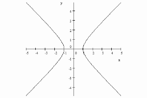
Figure 1: The graph corresponding to equation (1).

Next take a look at the following function

$$\sqrt{2}xy=1$$ (2)

Figure 2: The graph corresponding to equation (2).

It is not obvious to determine at sight the relation between the two prescriptions (1) and (2). However, when we plot the graph it is rather obvious that (2) also represent a hyperbole. Upon inspection, we see that graph 2 is like graph 1, but turned 45 degrees anti-clockwise. The graphs make clear what the mathematical prescriptions do not: that (1) and (2) represent the same geometrical object but seen through different eyes. When we say it is the same geometrical object, we mean that one can be obtained from the other employing only a combination of rotation, scaling and translation. This corresponds to our experience in the real world. When an observer moves through space, he may see an object at a different angle, a different size and in a different location, but it will still be the same object. There is a general mathematical method to see if two mathematical prescriptions of a quadratic form such as (1) and (2) determine the same geometrical object. First we have to associate a 2x2 matrix with the mathematical prescription. To do so, we first write the mathematical prescription in a canonical form

$$a_{11}x^{2}+2a_{12}xy+a_{22}y^{2}=1$$ (3)

The associated 2x2 matrix is a mathematical entity with 4 entries organized as a square:

$$A=\begin{pmatrix}a_{11}&a_{12}\\ a_{21}&a_{22}\end{pmatrix}$$ (4)

So $a_{11}$ is the coefficient of $x^{2},$ $a_{22}$ is the coefficient of $y^{2}$, $a_{12}$ is half the coefficient of $xy$ and $a_{21}$ half the coefficient of $xy.$ This means that $a_{12}=a_{21}.$ In general (that is, also for more than two free variables), the matrix of a quadratic form is symmetric. This means that if we interchange the rows and columns of $A,$ (this is the so-called transpose $A^{T}$ of that matrix) we get the same matrix:

$$A^{T}=A$$ (5)

Next we introduce a vector $\mathbf{x,}$ which is a shorthand for the two original variables $x$ and $y,$and its transpose $\mathbf{x}^{T}$:

$$\mathbf{x}=\begin{pmatrix}x\\ y\end{pmatrix}\text{ and }\mathbf{x}^{T}=\begin{pmatrix}x&y\end{pmatrix}$$ (6)

We are now in a position to write any (central) conic sections, i.e. the circle, the ellipse, the parabola and the hyperbole in the quadratic form:

$$\mathbf{x}^{T}A\mathbf{x}=1$$ (7)

For example, when employing the rules for matrix multiplication (which we will not give here), we get

$$\mathbf{x}^{T}A\mathbf{x}=\begin{pmatrix}x&y\end{pmatrix}\begin{pmatrix}1&0\\ 0&-1\end{pmatrix}\begin{pmatrix}x\\ y\end{pmatrix}=x1x+y(-1)y=1$$ (8)

which clearly represents (1), and

$$\begin{pmatrix}x&y\end{pmatrix}\begin{pmatrix}0&\sqrt{2}/2\\ \sqrt{2}/2&0\end{pmatrix}\begin{pmatrix}x\\ y\end{pmatrix}=x(\frac{\sqrt{2}}{2})y+x(\frac{\sqrt{2}}{2})y=1$$ (9)

which represents (2). Next we search for a way to identify the shape of the solutions independent of the actual form of the $x$’s and $y$’s. For this we diagonalize, that is transform it in such a way that only the entries $a_{11}$ and $a_{22}$ are different from zero. Of course, we are only allowed transformations of the matrix that leave the original geometrical object it represented intact. For an arbitrary matrix this is not possible, but for a symmetric 2x2 matrix, as is the case here, we can always bring it into a diagonal form by only applying a single rotation. If we applied the method of diagonalization (which we will not present here), we would find the diagonal form of the 2x2 matrix $A$ in (9) is precisely the 2x2 matrix in (8). In this new reference frame, obtained from the old by rotation, we can easily recognise the kind of geometrical object the quadratic form presents, because it is in its standard form. There is important terminology to remember here. The axes of the new frame of reference correspond to the eigenvectors of the matrix $A$. What is an eigenvector?

For a moment, let us forget about the original functions we are studying and just look at the following matrix equation:

$$A\mathbf{x}=\mathbf{x}^{\prime}$$ (10)

This equation tells us every vector $\mathbf{x}=(x,y)$ will, upon multiplication with the matrix $A,$ transform into a new vector $\mathbf{x}^{\prime}$. Of course it could be the case that for a certain special vector $\mathbf{x}_{0}$ this new vector $\mathbf{x}_{0}^{\prime}$ is just a multiple of the old vector $\mathbf{x}_{0}$:

$$A\mathbf{x}_{0}\mathbf{=\mathbf{x}_{0}^{\prime}=\lambda}_{0}\mathbf{x}_{0}$$ (11)

If this is the case, we say $\mathbf{x}_{0}$ is an eigenvector of the matrix $A$ and the (real or complex) number $\mathbf{\lambda}_{0}$ is its associated eigenvalue. For example, the eigenvalues of the matrix in (8) are $1$ and $-1$. Armed with this terminology we can make a summary of our observations.

Summary: The quadratic form (7) obtains its most simple (diagonal) form when described in a frame of reference whose axes are the vectors (11) that are left invariant (up to multiplication by a number) by the matrix (4) associated with the quadratic form. When presented in this form, the diagonal elements of the matrix $A$ are called the eigenvalues of $A$. The geometrical content of the quadratic form (7) can be determined directly from the eigenvalues of its associated matrix.

If we have this diagonalized form, we can easily recognise whether the geometrical object is a parabola or a hyperbole or an ellipse, because the diagonal form is just the standard function we learned for these objects in high school. If the eigenvalues of the matrix in (8) are $1$ and $-1$ (as is the case here), this means the geometrical object is a hyperbole. If both had been $+1$, it would have been a circle. If they had been two different positive numbers, it would have been an ellipse. When one of them is zero, but not both, we are dealing with a parabola.

Of course, the same results can be obtained using only elementary algebraic calculations, but the method presented here works for an arbitrary number of dimensions, not just for two, as long as we are only presenting a quadratic form. It is important to note that it works for vectors and matrices with complex entries too, but the condition (5) of symmetry is to be replaced with the corresponding complex notion, that of a self-adjoint matrix. Think of a self-adjoint matrix as simply a matrix that can be brought into diagonal form and for which the eigenvalues are all real. It turns out that an observable quantity in quantum mechanics is represented by a self-adjoint operator. Indeed, the same technique can be used to describe systems with a finite number of outcomes quantum mechanically, and the analogy is quite precise.

3.2 Incompatibility in analytic geometry

Suppose we have an equation such as

$$-\sqrt{2}x^{3}y+\sqrt{2}xy^{3}+\sqrt{2}xy+x^{2}-y^{2}=1$$ (12)

what geometrical object would this represent? After a simple calculation, we find that it is equivalent to

$$(x^{2}-y^{2}-1)(\sqrt{2}xy-1)=0$$ (13)

What is the solution of this equation? Well, it is of the general form $AB=0$ with $A=x^{2}-y^{2}-1$ and $B=\sqrt{2}xy-1.$ This equation is satisfied when either $A$ is zero, or $B$ is zero. So the equation is obviously satisfied when either (1) or (2) is satisfied. The complete solution of (13) is then the set of points $(x,y)$ that belongs to the first or the second hyperbole, and the graph of the horrible looking (13) is nothing but two graphs of (1) and (2) together. The relevant observation here, is that the basis that makes (1) diagonal (and hence takes the formula for the hyperbole in its standard form) does not make (2) diagonal, simply because the eigenvectors of the two are different. We can transform the form (12) such that either (1) is in standard form, or (2), but never the two simultaneously. We could say the two standard forms are incompatible in the sense that no single perspective can yield both simple forms at the same time. A similar situation occurs in the description of quantum systems.

3.3 Description and complementarity in quantum mechanics

Suppose we have a system that we seek to describe by quantum mechanics. The theory tells us the state of a physical system is represented by a vector, say $\psi$, living in an abstract Hilbert space $H$. Another fundamental postulate of quantum mechanics is that any quantity that we want to infer experimentally from that state $\psi$, whether it be its energy, its position or its momentum, is represented by a self-adjoint operator $A$. Quantum mechanics dictates furthermore that the outcome of the measurement will be one of the eigenfunctions of the operator, and that the probability of obtaining that result is the square of the norm of the coefficient that goes with the eigenvector which corresponds to the outcome. Furthermore, if the matrix $A$ represents the quantity we are interested in, and we want to know the expectation value $\langle A\rangle$ (a number representing the average physical value of $A$) when the system is in the state $\psi$, we have

$$\langle\psi|A|\psi\rangle=\langle A\rangle$$ (14)

We briefly indicate the meaning of the notation in (14). The quantity $\langle A\rangle$ on the right-hand side of equation (14) is just a number. We can always rescale the matrix so that the left-hand side of the equation equals one without altering the essential geometrical content . The so-called bra vector $\langle\psi|$ in (14) is the dual of its corresponding ket vector $|\psi\rangle$, just in the same way as $\mathbf{x}^{T}$ in (7) represents the dual of $\mathbf{x}$ for finite spaces. These are the fundamental postulates of simple, non-composite, non-relativistic quantum systems and to understand the geometrical meaning of the words in these postulates, we only need the analogy with analytic geometry. Indeed, Eq. (14) may look cumbersome to the reader who is unfamiliar with the bra-ket notation, but for observation of systems with only a finite number of outcomes, it is formally equivalent to the quadratic form (7):

$$\mathbf{x}^{T}A\mathbf{x}=1$$

According to the former section on analytic geometry, we already know how to find the eigenvectors and corresponding eigenvalues: we simply have to diagonalise the self-adjoint matrix that corresponds to that observable quantity. Just as in the case of analytic geometry, the matrix $P$ corresponding to a given operator, say its momentum $\hat{p}$, yields its “secrets” easily in a description that fixes the axes of reference to the eigenvectors of that same matrix: in its diagonal form, the probability of an outcome is simply the square of the corresponding diagonal element. Now we ask whether the same is true for the position of the system. Well of course, it is an axiom of quantum mechanics!. Simply calculate the eigenvectors of the matrix $Q$ that corresponds to the position operator $\hat{q}$ of a system, and draw your frame of reference there. Look again at what you have got, and you will only find diagonal entries from which you can immediately read the probability of obtaining a certain result. Now we may wonder: is the new frame of reference that diagonalizes $Q$, also a frame of reference that diagonalizes $P$? The answer depends on the relation between $P$ and $Q$. It is a mathematical theorem that if and only if $P$ and $Q$ (or their associated operators $\hat{p}$ and $\hat{q}$ ) commute, there exists a common frame of reference in which both are diagonal. But $P$ and $Q$ do not commute in quantum mechanics, and hence there is a problem with the simultaneous extraction of position and momentum information for a quantum mechanical system. Indeed, in quantum mechanics, we have the commutator relation:

$$\hat{p}\text{ }\hat{q}-\hat{q}\text{ }\hat{p}=\frac{ih}{2\pi}\hat{I}$$ (15)

in which $h$ is the famous constant of Planck and $\hat{I}$ the identity operator which is clearly different from zero . So we know from this equation (whatever the value at the right hand side was) that there does not exist a common frame of reference such that both $P$ and $Q$ are diagonal. Bohr introduced the notion of complementarity to describe this phenomenon. $Q$ and $P$ are like the inside and outside view of a house: both yield valuable information as to what a house is, but the better one can see the inside, the more one is neglecting the outside. Bohr coined the phrase that $P$ and $Q$ are complementary descriptions of the same system. The simultaneous extraction of $P$ and $Q$ information is hence limited by the uncertainty principle of Heisenberg, to which we will come back later. Many of the early gedanken experiments in the early history of quantum mechanics, and from the historic Solvay conference in 1927 in particular, can serve (and indeed were meant to serve) as an illustration of this principle [3].

4 Signal analysis

There is another field of scientific inquiry that has had to learn to deal with incompatible perspectives of the nature of the phenomenon; the field of signal analysis. The field of signal analysis is concerned with the extraction of information from a time-varying quantity which is called the signal. The signal can originate from very different sources. It can be electromagnetic, acoustic, optical or mechanical. It can contain various quantities and qualities of information. Needless to say, how to extract information depends on the way you look at things. Let us take an example. Suppose a sound technician is responsible for the music played by a live band at a party with a strict beginning and end in time and a strict limit to the amount of decibels that may be produced so that no neighbors are disturbed by the party. To make sure he starts and ends at the right moment, he checks, and if necessary adjusts his watch beforehand. At the moment the band starts, he lets the volume rise to an audible level that is still under the prescribed decibel limit and stops right before the announced end of the party. Take the music coming out of the speakers as the signal. The mathematical representation of this music as a time-varying quantity will allow him to do all that he needs. Given just this time-varying quantity, he could even have been in a remote place where he cannot hear the music and still perform the task he was given with a remote control. He merely needs to check that the signal starts after the prescribed time, stops before the prescribed ending, and make sure it does not exceed the given maximum volume. Suppose now however that the live music produces a feedback effect. The volume grows and an insistent, painful whistling tone is heard. If the sound technician is there, he will correct the problem, but if he is in a remote location with his remote control, he will simply lower the volume somewhat and assume everything is alright. The people attending the party will probably judge differently. The time varying quantity does not easily allow for the reading of frequency related information. If however, the sound technician made use of a spectral analyzer, he would have been able to correct even that problem remotely. The spectral analyzer performs a transformation of the signal. Rather than displaying the intensity of the signal in time, it yields the intensity of the various frequency bands heard within a given time interval. The feedback will be visible as a rapid and lasting rise of a small frequency band. Technically, the transform involved is called a short-time Fourier transform of the signal. It turns out that the operator corresponding to the Fourier transform does not commute with the operator that yields the intensity at every instant. So we see that the situation is quite similar to quantum mechanics from this point of view. In both situations, we are looking for an appropriate perspective to describe or extract the information, by transforming the system to a frame of reference that is constructed on the basis of the eigenvectors of the quantity that we seek to describe.

4.1 Quantum probability and signal analysis

The introduction of many of the definitions and methods used in signal analysis originated from similar developments in quantum mechanics. In a sense this is a curious historical fact, as it was originally accepted that quantum physics presents a fundamentally different theory than classical physics and the physics of signals is essentially classical. As physicists like to point out, quantum mechanics is inherently indeterministic, and signals are essentially deterministic. Whereas quantum physics describes the fundamental interactions in nature and is governed by Planck’s constant, signals are continuous in nature and no constant governs their behavior. Yet in the literature on signal analysis, see [4] and [5], we find the names of famous quantum physicists like Weyl (ordered operator algebra), Wigner (quasi-distribution), Heisenberg (uncertainty boxes) and Cohen (bilinear class). In 1946 Gabor, the inventor of the hologram and the atomic representations of signals, introduced the Heisenberg inequality in signal analysis [6]. Only two years later, Ville,[7] was to introduce a time–frequency distribution as a signal analytic tool that is formally equivalent to Wigner’s distribution in quantum mechanics [8]. The similarities between the two is of such extent, that apparently some concepts were invented independently in both subjects without reference to its parallel in the other subject. Although Ville constantly evokes language borrowed from quantum mechanics, the Ville distribution itself was originally given without reference to Wigner and the same occurred with the Rihaczek distribution,[9] that was historically preceded by the Margenau and Hill distribution in 1961 [4]. Sometimes researchers in quantum mechanics would cross the border to publish results useful to the signal analyst. We mention Cohen’s work, on bilinear and completely positive phase space distributions and the squeezed states of Caves,[11] and Man´ko,[12] that have found application in the construction of signals that are used in radar technology. To give the reader a taste of the extent of the overlap between the two fields, we sum up the main similarities. Both signals and quantum states are identified with vectors in a Hilbert space. Both see as operational quantities the modulus squared of these elements, which in signal analysis is called the energy density of the signal and in quantum mechanics the probability density of the entity. Both utilize the Fourier transform as the relationship between two of the most important operational quantities, time and frequency in signal analysis and position and momentum in quantum mechanics. As a consequence, both use the Heisenberg inequality and frequently employ non-commuting operators for observable quantities. Both fields employ the Wigner quasi-distribution as a phase space quasi-density.

4.2 The Fourier paradigm

Basic detection and error estimates can be given just from examining the major repetitive components of a signal. If major components in the signal tend to have a repetitive nature, one can average the signal over a large number of cycles. This technique is called time synchronous averaging and diminishes the noise content of the signal. Another very popular technique to acquire primitive frequency-related information of a signal $\phi(t)$, is to take the auto-correlation function, which is the average of the product $\phi(t)\phi(\tau+t).$ However, if the signal is too complex, these methods have their limitations in providing frequency related information. The cure, which marked the birth of modern mathematical signal analysis, dates back to Joseph Fourier’s (1768–1830) investigations into the properties of heat transfer in the early 1800’s [14]. Fourier conjectured that an arbitrary periodic function, even with discontinuities, could be expressed by an infinite sum of pure harmonic terms. The idea was ridiculed among many great scholars, but a large portion of mathematical analysis in the 19th and 20th centuries was dedicated to making the statements of Fourier precise and the Fourier transformation eventually became a tool of utmost importance in signal analysis, quantum physics and the theory of partial differential equations. In words, the Fourier theorem states that the sum of an infinite number of appropriate trigonometric functions, can be made to converge to any periodic function. Take a signal with period $2L$

$$\phi(t)=\phi(t+n2L),n=1,2,3,\ldots$$

Calculate the following quantities with $\omega=\frac{\pi}{L}$:

$$a_{0} = \frac{1}{L}\int_{-L}^{L}\phi(t)dt$$

$$a_{n} = \frac{1}{L}\int_{-L}^{L}\phi(t)\cos(n\omega t)dt$$

$$b_{n} = \frac{1}{L}\int_{-L}^{L}\phi(t)\sin(n\omega t)dt$$

Knowledge of the signal $\phi(t)$ obviously implies knowledge of the numbers $a_{n}$ and $b_{n},$ provided the integrals exist. But Fourier’s theorem states the far less obvious fact that, under mild assumptions, the converse also holds

$$\phi(t)=a_{0}/2+\sum_{n=1}^{+\infty}a_{n}\cos(n\omega t)+b_{n}\sin(n\omega t)$$

Knowledge of the numbers $a_{n}$ and $b_{n}$ implies complete knowledge of $\phi(t).$ The Fourier expansion is such a valuable tool because of its ability to decompose any periodic function (e.g. machine vibrations, sounds, heat cycles,…) by means of sines and cosines. As the reader may now appreciate, one can regard the sines and cosines as the eigenfunctions of the frequency operator. They form the orthonormal basis functions, the axes of the new frame of reference, and the coefficients of these orthonormal basis functions represent the contribution of the sine and cosine components in the signal. This allows the signal to be analyzed in terms of its frequency components. Rather than studying signals in their time domain, one could now study the characteristic frequencies of the phenomenon. A serious draw-back of the method is that only periodic signals can be represented. The Fourier paradigm was extended to cover non-periodic functions by means of the so called Fourier transform. To include non-periodic functions, we take the limiting case of the Fourier series when the period of the function goes to infinity. When we do this, we obtain the following formulas:

$$\Phi(\nu) = \int_{-\infty}^{+\infty}\phi(t)\exp(-2\pi i\nu t)dt$$ (16)

$$\phi(t) = \int_{-\infty}^{+\infty}\Phi(\nu)\exp(2\pi i\nu t)d\nu$$

We call $\Phi(\nu)$ the Fourier transform of $\phi(t),$ often written as $\mathcal{F}[\phi(t)]=$ $\Phi(\nu),$ and $\phi(t)$ is the inverse Fourier transform of $\Phi(\nu)$ written as $\mathcal{F}^{-1}[\Phi(\nu)]=\phi(t)$. The couple of functions $\{\phi(t),$ $\Phi(\nu)\}$ is called a Fourier pair. The drawback of this representation, as one can judge from the boundaries of the integral, is that the signal has to be known at all possible times, something that is never the case in applications. Of course, in an idealized situation, such as a quasi-monochromatic or a steady state description, the method yields true properties of the signal in question. But transitional regimes of signals are simply beyond the scope of this method. Even with this limitation, the importance of the consequences of (16) can hardly be overestimated. It was a source of inspiration to most advanced methods of transformation that eventually led to the field of wavelets, which have found wide spread use in almost all practical branches of contemporary applied science [5]. Let us therefore have a brief look at some of the properties of the Fourier pair (16).

4.3 Properties of Fourier pairs

We call the region were a function does not vanish (i.e. is not equal to zero), the support of that function. If the support of $\phi(t)$ is of finite width, then the width of the support of $\Phi(\nu)$ is infinite and vice versa. But even with unbounded support (i.e., when the support has infinite extension), a reciprocal relationship exists between $\phi(t)$ and $\Phi(\nu).$ To see this, assume the signal is normalized ($\int_{-\infty}^{+\infty}|\phi(t)|^{2}dt=1$) and that the center of gravity of both $\phi(t)$ and $\Phi(\nu)$ vanishes:

$$\int_{-\infty}^{+\infty}t|\phi(t)|^{2}dt=\int_{-\infty}^{+\infty}\nu|\Phi(\nu)|^{2}d\nu=0$$

This can always be realized by an appropriate choice of the axes. We define the following quantities:

$$\Delta t = \int_{-\infty}^{+\infty}t^{2}|\phi(t)|^{2}dt$$

$$\Delta\nu = \int_{-\infty}^{+\infty}\nu^{2}|\Phi(\nu)|^{2}dt$$

If $\phi(t)$ decays fast enough such that $t|\phi(t)|^{2}$ vanishes at infinity, the following relation follows from the Cauchy–Schwartz inequality:

$$\Delta t.\Delta\nu\geq\frac{1}{4\pi}$$

This relation is known in the literature on signal-analysis as the Heisenberg–Gabor uncertainty principle. The name is due to the fact that Gabor, an electrical engineer working on communication theory, discovered the relevance of this relationship to signal-analysis in 1946, about two decades after Heisenberg — one of the founding fathers of quantum physics — formulated the principle on physical grounds [6]. Weyl showed it to be a mathematical consequence of the fact that the corresponding operators are a Fourier pair [15]. And we see that indeed, the frequency and temporal descriptions of a signal yield complementary views of its information content. It should therefore come as no surprise that their respective operators do not commute. Instead of $\hat{t}$ $\hat{\nu}=\hat{\nu}$ $\hat{t},$ we have:

$$\hat{\nu}\text{ }\hat{t}-\hat{t}\text{ }\hat{\nu}=\frac{i}{2\pi}\hat{I}$$

Similar equations exist for the time and scale operators that are found in the literature on wavelets. This is to be compared with the equivalent relation for position and momentum in quantum mechanics (15):

$$\hat{q}\text{ }\hat{p}-\hat{p}\text{ }\hat{q}=\frac{ih}{2\pi}\hat{I}$$

where $h$ denotes Planck’s constant. This latter relation implies the well-known Heisenberg uncertainty relation:

$$\Delta q.\Delta p\geq\frac{h}{4\pi}$$

We see that, apart from Planck’s constant, the commutator and uncertainty relations have the same mathematical content when we apply the following substitution:

$$\hat{p} \rightsquigarrow \hat{\nu}$$

$$\hat{q} \rightsquigarrow \hat{t}$$

$$h \rightsquigarrow 1$$

With this basic vocabulary, it is easy to extend the list to include many more examples of corresponding quantities. We refer the interested reader to Ref. [10], p. 197.

5 Concluding remarks: The necessity of combining mutually incompatible perspectives.

We have seen that there are striking mathematical similarities between quantum mechanics and signal analysis. Historically, these mathematical analogies are the roots of the ongoing cross-fertilization between the two fields. Moreover, when we encounter a discussion in the literature that attempts to answer why this cross-fertilization has taken place, the similarity between the mathematics is invariably seen as the main source. There is no doubt that this analysis of the situation is correct, but it leaves the question why the similarities are there in the first place unanswered. Of course, the analogies could be purely coincidental. For example, both fields emerged from studies in the physics of heat. Quantum physics originated from the study of black body radiation, and signal analysis was born with Fourier’s study of heat processes. We believe this is indeed coincidental, as neither quantum physics, nor signal analysis deals primarily with the problems of heat transfer or radiation. On the other hand we believe the nature and origin of the similarities we have described is not coincidental, and we have given a metaphor from analytic geometry to support that thesis. The origin of the analogy that we identified from our metaphor is that, even though the state of a system (or signal) can be fully known, the extraction of measurable quantities (relevant information of signal) from a state requires taking a point of view, and not all points of view are compatible with one another. So we conjecture that the reason for the mathematical parallels is that both theories inherently contain a theory of observation. Complementarity arises in both fields because in some parts of reality there are mutually incompatible, but equally valid, perspectives of the same object. One cannot see the inside and outside of a house at the same time. A natural question to consider is then: When do we know when we have a sufficient number of views so that we are certain that we have seen “the full house”? The metaphor from analytic geometry regards “perspective” as the equivalent of “frame of reference”. We have elaborated that the frame constructed from the eigenvectors of the operator that represents the kind of information we are interested in yields the most simple description. So our question can now be translated as follows: What set of operators do we need to make sure that we have seen every aspect of the house? The most direct way of tackling that question, relies on Prugovečki’s concept of informational completeness within quantum mechanics [16]. A set of operators is called informationally complete if there is only one state compatible with the probabilities obtained from it. This means that for an informationally complete set of measurements, the state can be uniquely derived from the expectation values of these measurements. Moreover, the expectation value of any operator (i.e. any point of view) can be calculated as a simple average of functions of the outcome probabilities of the informationally complete set.

Now one can raise the question whether the whole phenomenon of complementarity cannot be avoided. If we take a sufficient number of compatible perspectives (i.e., commuting operators) can we obtain an informationally complete set? The answer is no. It was shown by Bush and Lahti [17], that no set of commuting observables is informationally complete! Complementarity is here to stay. This was intuitively accepted by most researchers in both fields, even though the result of Bush and Lahti is not widely known among quantum physicists, and largely unknown among signal analysts. Nevertheless, it is common knowledge among researchers in the field of theoretical signal analysis, that analyzing a signal in terms of the distribution in the non-commuting observables that are relevant, provides a much more revealing picture in many cases than, for example, the spectrogram or the signal together with its Fourier transform. One can show the spectrogram (and most other representations) to be informationally incomplete and the Wigner–Ville distribution to be informationally complete [13].

If our analysis makes sense, we should find that if one restricts the observations in quantum physics to the case of a single observable, that is to the results of essentially one experimental set-up, the results of the quantum probabilistic scheme can be reproduced by a classical probability model. It turns out that this is true. Hence the power of quantum statistical methods over classical probabilistic analysis is perhaps most obvious when dealing with expectation values and correlations of observables that do not commute. It is in this respect that quantum-like representations, be it a phase space representation or a density matrix, provide us with a statistically complete language for the incorporation of data from disjoint or incompatible measurements into a single state of the entity under observation. As a consequence, the conventional paradigm that quantum probability pertains to the micro-world and classical (Kolmogorovian) probability pertains to the macro-world is no longer tenable from this point of view. This is not because micro-physical principles of the entities under observation are at work, but because the relation between the possible ways in which we look at these phenomena is structurally isomorphic. But mutually incompatible perspectives are to be found in many areas that are of scientific interest. What about the social implications of interactions between cultures with incompatible value systems? What about the well-known graphical figures that yield one gestalt or another (but never both at the same time) depending on how they are looked at? A sentence may be deemed innocent within one context, but disturbing in another. A single note can make one chord cheerful and another chord sad. One cannot hope that investigations in these areas will yield precise quantitative statements any time soon in the same way as we have in engineering or physics. Nevertheless, the lesson that it is only together that these incompatible perspectives give an informationally complete picture may well be still valid.

References

- [1] W. Heisenberg, Physics and Philosophy. Penguin books (1990).
- [2] C. W. Helstrom, Elements of Signal detection and estimation. Prentice Hall, Englewood (1995).
- [3] J. A. Wheeler and W. H. Zurek, Quantum theory and measurement. Princeton (1983).
- [4] P. Flandrin, Time–frequency / Time-scale analysis. Wavelet analysis and its applications vol. 10, Academic Press, London (1999).
- [5] S. Mallat, A wavelet tour of signal processing. Academic Press, London (1998).
- [6] D. Gabor, Theory of communications. J. Inst. Elect. Eng., London, 93, 429–457 (1943).
- [7] J. Ville, Theorié et applications de la notion de signal analytique. Cables et transmission, 2A(1): 61–74 (1948).
- [8] E. P. Wigner, On the quantum mechanical correction for thermodynamic equilibrium. Phys. Rev., 40: 749–759 (1932).
- [9] A. W. Rihaczek, Signal energy distribution in time and frequency. IEEE Trans. Info. Theory, 14, 369–374 (1968).
- [10] L. Cohen, Time–frequency analysis. Prentice Hall (1995).
- [11] C. M. Caves, Defense of the standard quantum limit for free-mass position. Phys. Rev. Lett., 54, 2465–2468 (1985).
- [12] V. I. Man’ko, Squeezed states, quantum fields, and uncertainty relations. Proceedings of the 7th international workshop on Nuclear theory, Rila, Bulgaria, 8–13 June (1987).
- [13] F. E. Schroeck, Quantum Mechanics on Phase space. Kluwer Academic Publishers, Dordrecht (1996).
- [14] J. Fourier, Theorié analytique de la chaleur. Paris, Chez Firmin Didot, Père et Fils (1822).
- [15] H. Weyl, Gruppentheorie und Quantenmechanik. Hirzel, Leipzig (1928).
- [16] E. Prugovečki, Information-theoretical aspects of quantum measurement. Int. J. Theor. Phys., 16, 321–331 (1977).
- [17] P. Bush and P.J. Lahti, The determination of the past and the future of a physical system in quantum mechanics. Found. Phys., 19, 633 (1989).