Conditional generation of arbitrary single-mode quantum states of light
by repeated photon subtractions

Abstract

We propose a scheme for the conditional generation of arbitrary finite superpositions of (squeezed) Fock states in a single mode of a traveling optical field. The suggested setup requires only a source of squeezed states, beam splitters, strong coherent beams, and photodetectors with single-photon sensitivity. The method does not require photodetectors with a high efficiency nor with a single-photon resolution.

I Introduction

During recent years it has been widely recognized that non-classical states of light represent a valuable resource for numerous applications ranging from ultra-high precision measurements Yurke86 ; Hillery93 ; Dowling98 to quantum lithography Boto00 ; Bjork01 and quantum information processing Bouwmeester . It is often desirable to generate nonclassical states in traveling optical modes, as opposed to the cavity QED experiments where the generated state is confined in a cavity and can be probed only indirectly. Many ingenious schemes have been proposed and experimentally demonstrated to generate the single-photon states Lvovsky01 ; Zavatta04 and various multiphoton entangled states such as the GHZ states Pan00 , cluster states Walther05 , and the so-called NOON states Gerry02 ; Fiurasek02 ; Kok02 ; Mitchell04 ; Eisenberg04 .

Considerable attention has been also devoted to the preparation of arbitrary single-mode states Dakna99 ; Clausen01 ; Villas-Boas01 ; Zou04 and, in particular, the Schrödinger cat-like superpositions of coherent states Dakna97 ; Lund04 which can represent a valuable resource for quantum information processing Jeong02 ; Ralph03 . Experimental generation of arbitrary superpositions of vacuum and single-photon states has been accomplished using a parametric down-conversion with input signal mode prepared in a coherent state Resch02 , employing the quantum scissors scheme Pegg98 ; Babichev03 or conditioning on homodyne measurements on one part of a non-local single photon in two spatial modes Babichev04 . It is, however, very difficult to extend these experiments to superpositions involving also two or more photons. The known schemes for conditional generation of arbitrary superpositions of Fock states require single-photon sources and/or highly efficient detectors with single photon resolution which represents a formidable experimental challenge.

In this paper, we propose a novel state preparation scheme, which does not require single-photon sources and can operate with high fidelity even with low-efficiency detectors that only distinguish the presence or absence of photons. Our scheme is inspired by the proposal of Dakna et al. Dakna99 who showed that an arbitrary single-mode state can be engineered starting from vacuum by applying a sequence of displacements and single-photon additions. Our crucial observation is that if the initial state is a squeezed vacuum, then the single-photon addition can be replaced with single-photon subtraction Opatrny00 ; Kim04 , which is much more practicable. Indeed, a single-photon subtraction can be achieved by diverting a tiny faction of the beam with a beam splitter towards a photodetector, so that a click means that a photon has been subtracted from the beam (this process becomes exact for a transmittance tending to one). In fact, the single-photon subtraction from a squeezed vacuum has already been experimentally demonstrated Wenger04 , which provides a strong evidence for the practical feasibility of our scheme. We note that the photon subtraction is an extremely useful tool that allows to generate states suitable for the tests of Bell inequality violation with balanced homodyning Garcia04 ; Nha04 , can be used to improve the performance of dense coding Kitagawa05 , and forms a crucial element of the entanglement distillation schemes for continuous variables Browne03 .

The present paper is organized as follows. In Section II, we explain the mechanism of state generation on the simplest non-trivial example of preparing a squeezed superposition of vacuum and single-photon states. Our setup then consists of two displacements and one conditional photon subtraction. We present the details of the calculation of the Wigner function of the generated state for a realistic setup involving imperfect photon subtraction (obtained with imperfect detectors and beam splitters with a non-unity transmittance). In order to evaluate the performance of the scheme, we investigate the achieved fidelity and the preparation probability for various target states. In Section III, we extend the scheme to the generation of an arbitrary single-mode state and show how to calculate the displacements that need to be applied during the state preparation. As an illustration, we consider the generation of several states which are squeezed superpositions of vacuum, single-photon, and two-photon Fock states. Finally, the conclusions are drawn in Section IV.

II Generation of a squeezed superposition of $|0\rangle$ and $|1\rangle$

In this section, we introduce our setup for the generation of an arbitrary squeezed superposition of vacuum and single-photon state, which consists of two displacements with a photon subtraction in between, as schematically sketched in Fig. 1. This setup represents a basic building block of our universal scheme: as shown in Section III, any squeezed superposition of the first $N+1$ Fock states can be generated from a single-mode squeezed vacuum by a displacement followed by a sequence of $N$ photon subtractions and displacements.

II.1 Pure-state description

We first provide a simplified pure-state description of the setup, assuming perfect detectors with single-photon resolution, which will give us an insight into the mechanism of state generation. We will show that conditionally on observing a click of the photodetector PD, the setup produces a squeezed superposition of vacuum and single-photon states,

$$|\psi\rangle_{\mathrm{target}}=S(s)[c_{0}|0\rangle+c_{1}|1\rangle],$$ (1)

where $S(s)=\exp[s(a^{\dagger 2}-a^{2})/2]$ denotes the squeezing operator, and $a$ ($a^{\dagger}$) is the annihilation (creation) operator.

Our state engineering procedure starts with a single-mode squeezed vacuum state, which is generated in an optical parametric amplifier (OPA),

$$S(s_{\mathrm{in}})|0\rangle=\frac{1}{\sqrt{\cosh(s_{\mathrm{in}})}}\sum_{n=0}^{\infty}\frac{\sqrt{(2n)!}}{2^{n}n!}[\tanh(s_{\mathrm{in}})]^{n}|2n\rangle,$$ (2)

where $s_{\mathrm{in}}$ denotes the initial squeezing constant. The single-mode squeezed vacuum passes through three highly transmitting beam splitters, which realize a sequence of a displacement followed by a single-photon subtraction and another displacement. The state is displaced by combining it on a highly unbalanced beam splitter BS_D with transmittance $T_{D}>99$% with a strong coherent state $|\alpha/r_{D}\rangle$, where $r_{D}=\sqrt{R_{D}}$ and $R_{D}=1-T_{D}$ is the reflectance of BS_D Paris96 . In the limit $T_{D}\rightarrow 1$, the output beam is displaced by the amount $\alpha$. This method has been used, e.g., in the continuous-variable quantum teleportation experiments Furusawa98 . For the sake of simplicity, we shall assume that $T_{D}=1$ and the displacement operation is exact. The conditional single-photon subtraction requires a highly unbalanced beam splitter BS with transmittance $T$, followed by a photodetector PD placed on the auxiliary output port. A successful photon subtraction is heralded by a click of the detector. In the limit $T\rightarrow 1$, the most probable event leading to a click of the detector is that exactly a single photon has been reflected from the beam splitter. The probability of removing two or more photons is smaller by a factor of $1-T$ and becomes totally negligible in the limit $T\rightarrow 1$. The conditional single-photon subtraction can be described by the non-unitary operator

$$X=t^{n}r\,a,$$ (3)

where $n=a^{\dagger}a$ is the photon-number operator, while $t=\sqrt{T}$ and $r=\sqrt{1-T}$ denote the amplitude transmittance and reflectance of BS, respectively.

Figure 1: Proposed experimental setup for generating $|\psi\rangle=S(s)[c_{0}|0\rangle+c_{1}|1\rangle]$. An optical parametric amplifier (OPA) generates a single-mode squeezed vacuum state which then propagates through three highly unbalanced beam splitters BS_D, BS, and BS_D, which realize a sequence of two displacements interspersed with one conditional photon subtraction. Successful state preparation is heralded by a click of the photodetector PD.

The input-output transformation corresponding to the sequence of operations in Fig. 1 reads

$$|\psi\rangle_{\mathrm{out}}=D(\alpha_{2})XD(\alpha_{1})S(s_{\mathrm{in}})|0\rangle,$$ (4)

where $D(\alpha)=\exp(\alpha a^{\dagger}-\alpha^{\ast}a)$ is the displacement operator. We will show later on how the displacements $\alpha_{1}$ and $\alpha_{2}$ depend on the target state (1), as well as how the initial squeezing $s_{\mathrm{in}}$ depends on the target squeezing $s$ for a given transmittance $T<1$. But, to make it simple, let us assume first that $T=1$ and $\alpha_{1}=-\alpha_{2}=\alpha$. Then, using $D(\alpha)^{\dagger}aD(\alpha)=a+\alpha$, the conditionally generated state can be written as

$$|\psi\rangle_{\mathrm{out}}=(a+\alpha)S(s_{\mathrm{in}})|0\rangle.$$ (5)

Taking into account that $a$ and $a^{\dagger}$ transform under the squeezing operation according to

$$S^{\dagger}(s)aS(s)=a\cosh(s)+a^{\dagger}\sinh(s),$$

$$S^{\dagger}(s)a^{\dagger}S(s)=a^{\dagger}\cosh(s)+a\sinh(s),$$ (6)

we obtain

$$|\psi\rangle_{\mathrm{out}} = S(s_{\mathrm{in}})[a\cosh(s_{\mathrm{in}})+a^{\dagger}\sinh(s_{\mathrm{in}})+\alpha]|0\rangle$$ (7)

$$= S(s_{\mathrm{in}})(\sinh(s_{\mathrm{in}})|1\rangle+\alpha|0\rangle).$$

We can see that by setting $\alpha=(c_{0}/c_{1})\sinh(s_{\mathrm{in}})$, we obtain the target state (1). This simple analysis illustrates the principle of operation of the scheme shown in Fig. 1. However, the limit $T=1$ is unphysical, because the probability of successful state generation vanishes when $T\rightarrow 1$. Let us now take into account $T<1$.

In order to simplify the expression (4), we first rewrite all displacement operators in a normally-ordered form, $D(\alpha)=e^{-|\alpha|^{2}/2}e^{\alpha a^{\dagger}}e^{-\alpha^{\ast}a}$, and we obtain

$$|\psi\rangle_{\mathrm{out}}\propto e^{\alpha_{2}a^{\dagger}}e^{-\alpha_{2}^{\ast}a}\,t^{n}\,a\,e^{\alpha_{1}a^{\dagger}}e^{-\alpha_{1}^{\ast}a}S(s_{\mathrm{in}})|0\rangle.$$ (8)

Next, we propagate the operator $t^{n}$ to the right by using the relations

$$t^{n}e^{\alpha^{\ast}a}=e^{\alpha^{\ast}a/t}t^{n},\qquad t^{n}e^{\alpha a^{\dagger}}=e^{t\alpha a^{\dagger}}t^{n}.$$ (9)

After these algebraic manipulations we obtain

$$|\psi\rangle_{\mathrm{out}}\propto e^{\alpha_{2}a^{\dagger}}a\,e^{t\alpha_{1}a^{\dagger}}e^{-[\alpha_{2}^{\ast}+\alpha_{1}^{\ast}/t]a}\,t^{n}S(s_{\mathrm{in}})|0\rangle.$$ (10)

Note that we have also moved to the right the operator $e^{-\alpha_{2}^{\ast}a}$ and used the fact that $e^{\alpha a^{\dagger}}e^{\beta^{\ast}a}=e^{-\alpha\beta^{\ast}}e^{\beta^{\ast}a}e^{\alpha a^{\dagger}}$.

The combined action of the operators $t^{n}S(s_{\mathrm{in}})$ on vacuum produces a single-mode squeezed vacuum state (2) just as without applying $t^{n}$, only with a lower squeezing constant $s$ satisfying $\tanh(s)=t^{2}\tanh(s_{\mathrm{in}})$. Thus, we can write

$$t^{n}S(s_{\mathrm{in}})|0\rangle\propto S(s)|0\rangle.$$ (11)

Finally, we move the operator $e^{\alpha_{2}a^{\dagger}}$ to the right, using the formula $e^{\alpha_{2}a^{\dagger}}a=(a-\alpha_{2})\,e^{\alpha_{2}a^{\dagger}},$ which results in

$$|\psi\rangle_{\mathrm{out}}\propto(a-\alpha_{2})\,e^{\delta a^{\dagger}}e^{-\gamma^{\ast}a}S(s)|0\rangle,$$ (12)

where $\delta=\alpha_{2}+t\alpha_{1}$ and $\gamma=\alpha_{2}+\alpha_{1}/t$. With the help of Eq. (6), we can write,

$$e^{\delta a^{\dagger}}e^{-\gamma^{\ast}a}S(s)|0\rangle\propto S(s)e^{[\delta\cosh(s)-\gamma^{\ast}\sinh(s)]a^{\dagger}}|0\rangle,$$ (13)

which is a state with a generally non-zero coherent displacement. This displacement vanishes provided that $\alpha_{1}$ and $\alpha_{2}$ satisfy

$$(\alpha_{2}+t\alpha_{1})\cosh(s)=(\alpha_{2}^{\ast}+\alpha_{1}^{\ast}/t)\sinh(s).$$ (14)

If the condition (14) holds, then the output reads

$$|\psi\rangle_{\mathrm{out}} \propto (a-\alpha_{2})\,S(s)|0\rangle$$ (15)

$$\propto S(s)[a^{\dagger}\sinh(s)-\alpha_{2}]|0\rangle.$$

where we have moved the squeezing operator to the left using Eq. (6). The desired squeezed superposition of the first two Fock states (1) can then be obtained by choosing

$$\alpha_{2} = -\frac{c_{0}}{c_{1}}\sinh(s),$$ (16)

$$\alpha_{1} = t\frac{[\tanh^{2}(s)-t^{2}]\alpha_{2}+(t^{2}-1)\tanh(s)\alpha_{2}^{\ast}}{t^{4}-\tanh^{2}(s)},$$ (17)

where the displacement $\alpha_{1}$ is determined from the condition (14). Note that we may assume that the coefficient $c_{1}$ of the Fock state $|1\rangle$ is non-zero; otherwise, no photon subtraction is needed to generate the target state.

It should be emphasized that the generated state with our scheme is a squeezed superposition of Fock states. In principle, this squeezing could be removed by sending the conditionally generated state (15) through a squeezer $S(-s)$. However, in many cases, the squeezing may not be an obstacle or may even represent an advantage, such as in the generation of Schrödinger cat states $|\alpha\rangle-|-\alpha\rangle$ which can be for small $|\alpha|$ very well approximated by a squeezed single-photon state $S(s)|1\rangle$ Lund04 ; Kim04 .

II.2 Realistic model

We shall now present a more realistic description of the proposed scheme taking into account that the photodetectors exhibit only single-photon sensitivity, but cannot resolve the number of photons in the mode, and have a detection efficiency $\eta<1$. Such detectors have two outcomes, either a click or a no-click. We model this detector as a sequence of a beam splitter with transmittance $\eta$ followed by an idealized detector which performs a projection onto the vacuum and the rest of the Hilbert space, $\Pi_{0}=|0\rangle\langle 0|$ (no click), $\Pi_{1}=\openone-|0\rangle\langle 0|$ (a click).

Similarly as in Ref. Garcia04 , it is convenient to work in the phase-space representation and consider the transformation of Wigner functions. The setup in Fig. 1 involves two modes, the principal mode A and an auxiliary mode B. The Gaussian Wigner function of the initial state of mode A after the first displacement reads

$$W_{G}(r_{A};\Gamma_{A},d_{A})=\frac{\sqrt{\det\Gamma_{A}}}{\pi}e^{-(r_{A}-d_{A})^{T}\Gamma_{A}(r_{A}-d_{A})},$$ (18)

where $r_{A}=(x_{A},p_{A})^{T}$ is the vector of quadratures of mode A and $d_{A}=z_{1}\equiv\sqrt{2}(\Re\alpha_{1},\Im\alpha_{1})^{T}$ is the displacement. The matrix $\Gamma_{A}$ is the inverse of the covariance matrix $\gamma_{A}$. Initially, the mode A is in a squeezed vacuum state and the covariance matrix is diagonal, $\gamma_{A}=\mathrm{diag}(e^{2s_{\mathrm{in}}},e^{-2s_{\mathrm{in}}})$.

In a second step, the modes A and B are mixed on an unbalanced beam splitter BS and then mode B subsequently passes through a (virtual) beam splitter of transmittance $\eta$ which models the imperfect detection with efficiency $\eta$. This transformation is a Gaussian completely positive (CP) map $\mathcal{M}$, and the resulting state of modes A and B is still a Gaussian state with the Wigner function

$$W_{AB}(r_{AB})=\frac{\sqrt{\det\Gamma_{AB}}}{\pi^{2}}e^{-(r_{AB}-d_{AB})^{T}\Gamma_{AB}(r_{AB}-d_{AB})},$$ (19)

where $r_{AB}=(x_{A},p_{A},x_{B},p_{B})^{T}$. The vector of the first moments $d_{AB}=(d_{A},d_{B})^{T}$ and the covariance matrix $\gamma_{AB}=\Gamma_{AB}^{-1}$ can be expressed in terms of the initial parameters of mode $A$ before the mixing on BS (i.e., $z_{1}$ and $\gamma_{A}$) as follows:

$$d_{AB} \equiv \left(\begin{array}[]{c}d_{A}\\ d_{B}\end{array}\right)=S\left(\begin{array}[]{c}z_{1}\\ 0\end{array}\right),$$ (24)

$$\gamma_{AB} = S(\gamma_{A}\oplus I_{B})S^{T}+G,$$ (25)

where $S=S_{\eta}S_{BS}$, $S_{\eta}=I_{A}\oplus\sqrt{\eta}I_{B}$ and $G=0_{A}\oplus(1-\eta)I_{B}$ model the inefficient photodetector, and $S_{BS}$ is a symplectic matrix which describes the coupling of the modes $A$ and $B$ on an unbalanced beam splitter BS,

$$S_{BS}=\left[\begin{array}[]{cccc}t&0&r&0\\ 0&t&0&r\\ -r&0&t&0\\ 0&-r&0&t\\ \end{array}\right].$$ (26)

After the photon subtraction, the density matrix $\rho_{A,\mathrm{out}}$ of mode $A$ conditioned on a click of the photodetector PD measuring the auxiliary mode B becomes

$$\rho_{A,\mathrm{out}}=\mathrm{Tr}_{B}[\rho_{AB}(\openone_{A}\otimes\Pi_{1,B})],$$ (27)

where $\mathrm{Tr}_{B}$ denotes a partial trace over mode B, and $\rho_{AB}$ is the two-mode density matrix of the Gaussian state characterized by the Wigner function (19). Then, after the second displacement of $z_{2}\equiv\sqrt{2}(\Re\alpha_{2},\Im\alpha_{2})^{T}$, the Wigner function of mode A can be written as a linear combination of two Gaussian functions (18), namely

$$W(r)\,P=C_{1}W_{G}(r;\Gamma_{1},d_{1})+C_{2}W_{G}(r;\Gamma_{2},d_{2}),$$ (28)

where $P$ is the probability of successful generation of the target state. The expression (28) can be derived by rewriting Eq. (27) in the Wigner representation. One uses the fact that the Wigner function of the POVM element $\Pi_{1,B}$ is a difference of two Gaussian functions,

$$W_{\Pi_{1}}(r)=\frac{1}{2\pi}-\frac{1}{\pi}e^{-x^{2}-p^{2}},$$ (29)

and that the trace of the product of two operators can be evaluated by integrating the product of their Wigner representations over the phase space.

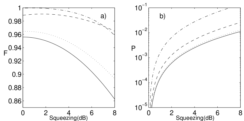
Figure 2: (a) Fidelity between the generated state and the target state and (b) probability of successful generation as a function of the squeezing $s_{\mathrm{in}}$ for the four target states (34) (solid line), (35) (dashed line), (36) (dot-dashed line) and (37) (dotted line), with $T=0.95$ and $\eta=0.25$.

To define the matrices and vectors appearing in Eq. (28), we first divide the matrix $\Gamma_{AB}=\gamma_{AB}^{-1}$ into four sub-matrices with respect to the $A|B$ splitting,

$$\Gamma_{AB}=\left[\begin{array}[]{cc}\Upsilon_{A}&\sigma\\ \sigma^{T}&\Upsilon_{B}\end{array}\right].$$ (30)

The correlation matrix $\Gamma_{1}$ and the displacement $d_{1}$ appearing in the first term on the right-hand side of Eq. (28) are given by

$$\Gamma_{1} = \Upsilon_{A}-\sigma\Upsilon_{B}^{-1}\sigma^{T},$$

$$d_{1} = d_{A}+z_{2},$$

$$C_{1} = 1.$$ (31)

Similarly, the formulas for the parameters of the second term read

$$\Gamma_{2} = \Upsilon_{A}-\sigma\tilde{\Upsilon}_{B}^{-1}\sigma^{T},$$

$$d_{2} = d_{A}+\Gamma_{2}^{-1}\sigma\tilde{\Upsilon}_{B}^{-1}d_{B}+z_{2},$$

$$C_{2} = -2\sqrt{\frac{\det(\Gamma_{AB})}{\det(\Gamma_{2})\det(\tilde{\Upsilon}_{B})}}\exp\left[-d_{B}^{T}Md_{B}\right],$$ (32)

where $\tilde{\Upsilon}_{B}=\Upsilon_{B}+I$ and

$$M=\Upsilon_{B}\tilde{\Upsilon}_{B}^{-1}-\tilde{\Upsilon}_{B}^{-1}\sigma^{T}\Gamma_{2}^{-1}\sigma\tilde{\Upsilon}_{B}^{-1}.$$ (33)

Since all the Wigner functions in Eq. (28) are normalized, the probability of a successful state generation can be calculated simply as the sum $P=C_{1}+C_{2}$.

II.3 Examples

In order to illustrate our method, let us consider the preparation of the following four squeezed superpositions of $|0\rangle$ and $|1\rangle$ states,

$$|\psi_{1}\rangle = S(s)|1\rangle,$$ (34)

$$|\psi_{2}\rangle = S(s)\frac{1}{\sqrt{2}}(|0\rangle+|1\rangle),$$ (35)

$$|\psi_{3}\rangle = S(s)\frac{1}{\sqrt{10}}(3|0\rangle+|1\rangle),$$ (36)

$$|\psi_{4}\rangle = S(s)\frac{1}{\sqrt{10}}(|0\rangle+3|1\rangle).$$ (37)

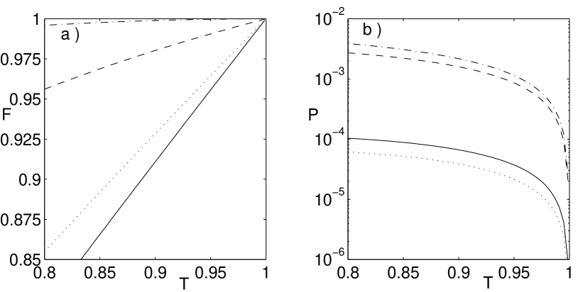
Figure 3: (a) Fidelity between the generated state and the target state and (b) probability of successful generation as a function of $T$ for the four target states (34)–(37). The curves are plotted considering the optimal squeezing $s_{\mathrm{in}}$ for each state, namely $0.50$ dB for state (34) (solid line), $1.66$ dB for state (35) (dashed line), $0.85$ dB for state (36) (dot-dashed line), and $0.36$ dB for state (37) (dotted line). The curves are plotted for $\eta=0.25$.

The fidelity of the generated state for the target states (34)–(37) is plotted in Fig. 2(a) as a function of squeezing. We can see that the conditionally prepared states are close to the desired states and their optimum fidelities are reached for a low initial squeezing (below $2$ dB), which is experimentally accessible. Although it is hardly visible in Fig 2(a), there is typically a non-zero optimal value of the squeezing, giving the highest fidelity. As shown in Fig. 2(b) the increase of the squeezing improves the probability of successful generation of the target state. A comparison of Fig. 2(a) with Fig. 2(b) reveals a clear trade-off between the achievable fidelity and the preparation probability.

Figure 3(a) shows the dependence of the fidelity on the beam splitter transmittance $T$, considering the optimal squeezing for each of the states. (Note that for state (34), we could not find numerically the optimum squeezing, so we arbitrarily chose $s_{\mathrm{in}}=0.50$ dB as an optimal value in other to keep a reasonable generation probability.) We see that as $T$ approaches unity, the fidelity gets arbitrarily close to unity, while the probability of successful state generation $P\propto(1-T)\,\eta$ decreases, as shown in Fig. 3(b). The value $T=0.95$ used in Fig. 2 seems to be a reasonable compromise between the success rate ($P\approx 10^{-3}$ or $P\approx 10^{-4}$ depending on the target state) and the fidelity, $F\gtrsim 0.95$%.

We also have studied the dependence of the fidelity on the detection efficiency $\eta$. The numerical results are shown in Fig. 4(a), where we can see that the scheme is very robust in the sense that the fidelity almost does not depend on $\eta$. Fidelities above $95$% could be reached even with $\eta$ of the order of a few percent if $T$ is high enough. This is in agreement with the findings of Ref. Garcia04 . However, a low $\eta$ reduces the preparation probability, as shown in Fig. 4(b).

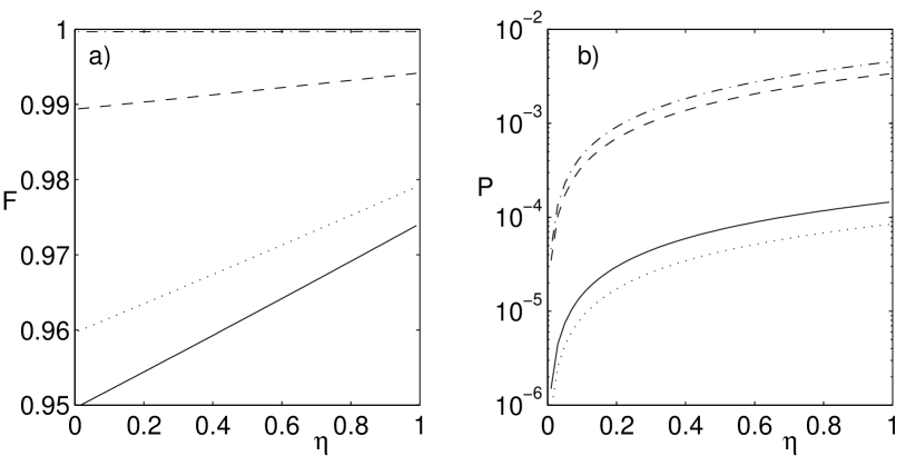
Figure 4: (a) Fidelity between the generated state and the target state and (b) probability of successful generation as a function of $\eta$ for the four target states (34)–(37). The curves are plotted considering the optimal squeezing $s_{\mathrm{in}}$ for each state, namely $0.50$ dB for state (34) (solid line), $1.66$ dB for state (35) (dashed line), $0.85$ dB for state (36) (dot-dashed line), and $0.36$ dB for state (37) (dotted line). The curves are plotted for $T=0.95$.

III Arbitrary single-mode squeezed state

In the preceding section, we have demonstrated that the combination of two displacements and a photon subtraction allows us to build any squeezed superposition of $|0\rangle$ and $|1\rangle$ states. In this section, we shall generalize this procedure to any squeezed superposition of the first $N+1$ Fock states,

$$|\psi\rangle_{\mathrm{target}}=S(s)\sum_{n=0}^{N}c_{n}|n\rangle,$$ (38)

and show that it can be prepared from a squeezed vacuum by applying a sequence of $N+1$ displacements interspersed with $N$ photon subtractions, as shown in Fig. 5.

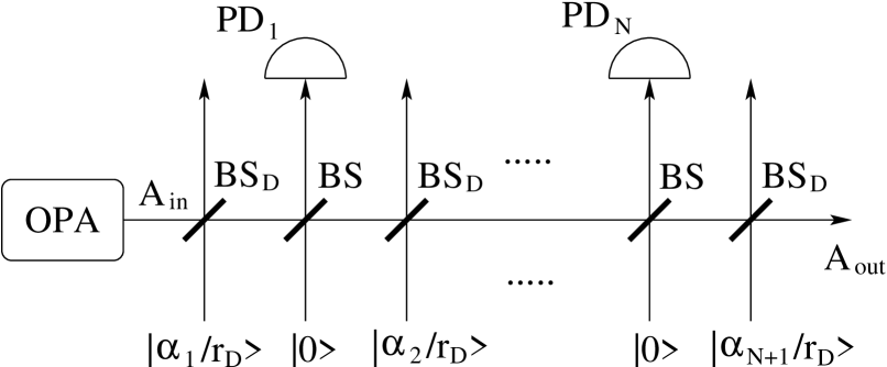
Figure 5: Proposed experimental setup. An optical parametric amplifier (OPA) generates a single-mode squeezed vacuum state which then propagates through $2N+1$ highly unbalanced beam splitters BS_D and BS, which realize a sequence of $N+1$ displacements interspersed with $N$ conditional photon subtractions. Successful state preparation is heralded by clicks of all $N$ photodetectors PD_k.

III.1 Pure-state description

As in the preceding section, we first provide a simplified pure-state description of the setup, assuming perfect detectors with single-photon resolution. This will allow us to determine the dependence of the coherent displacements $\alpha_{j}$ on the target state (38). Generalizing the procedure presented in the preceding section, the input-output transformation corresponding to the sequence of operations in Fig. 5 reads

$$|\psi\rangle_{\mathrm{out}}=D(\alpha_{N+1})XD(\alpha_{N})X\ldots D(\alpha_{2})XD(\alpha_{1})S(s_{\mathrm{in}})|0\rangle.$$ (39)

In order to simplify this expression, we first rewrite all displacement operators in a normally-ordered form and then move all the operators $t^{n}$ to the right using the relations (9). This results in the substitution $\alpha_{j}\rightarrow\alpha_{j}t^{N+1-j}$ and $\alpha_{j}^{\ast}\rightarrow\alpha_{j}^{\ast}t^{j-N-1}$ in the exponents. Next, we propagate all the exponential operators $e^{-t^{j-N-1}\alpha_{j}^{\ast}a}$ to the right,

$$|\psi\rangle_{\mathrm{out}}\propto e^{\alpha_{N+1}a^{\dagger}}ae^{t\alpha_{N}a^{\dagger}}a\ldots ae^{t^{N}\alpha_{1}a^{\dagger}}e^{-\gamma^{\ast}a}t^{Nn}S(s_{\mathrm{in}})|0\rangle,$$ (40)

where $\gamma=\sum_{j=1}^{N+1}\alpha_{j}t^{j-N-1}$. The combined action of the operators $t^{Nn}S(s_{\mathrm{in}})$ on the vacuum produces a single-mode squeezed vacuum state, $t^{Nn}S(s_{\mathrm{in}})|0\rangle\propto S(s)|0\rangle$, where $\tanh(s)=t^{2N}\tanh(s_{\mathrm{in}})$. After some algebraic manipulations we get

$$|\psi\rangle_{\mathrm{out}}\propto S(s)\prod_{j=1}^{N}(a\cosh(s)+a^{\dagger}\sinh(s)-\beta_{j})|0\rangle,$$ (41)

where

$$\beta_{j}=\sum_{k=j+1}^{N+1}\alpha_{k}t^{N+1-k}.$$ (42)

The formula (41) is valid provided that the overall displacement is zero. This corresponds to the constraint

$$\cosh(s)\sum_{j=1}^{N+1}\alpha_{j}t^{N+1-j}=\sinh(s)\sum_{j=1}^{N+1}\alpha_{j}^{\ast}t^{j-N-1}\,,$$ (43)

which generalizes condition (14).

We now prove that an arbitrary superposition of the first $N+1$ Fock states $\sum_{n=0}^{N}c_{n}|n\rangle$ can be expressed as $\prod_{j=1}^{N}(A-\beta_{j})|0\rangle\equiv\sum_{k=0}^{N}h_{k}A^{k}|0\rangle$, where $A=a\cosh(s)+a^{\dagger}\sinh(s)$ and $h_{k}$ are the coefficients of the characteristic polynomial whose roots are $\beta_{j}$. From the condition

$$\sum_{k=0}^{N}h_{k}A^{k}|0\rangle=\sum_{n=0}^{N}c_{n}|n\rangle,$$ (44)

we can immediately determine the coefficients $h_{N}$ and $h_{N-1}$, because only the term $A^{N}$ gives rise to $a^{\dagger N}$ and, similarly, only the expansion of $A^{N-1}$ contains $a^{\dagger N-1}$. We thus get equations

$$h_{N}=\frac{c_{N}\sinh^{-N}(s)}{\sqrt{N!}},\qquad h_{N-1}=\frac{c_{N-1}\sinh^{1-N}(s)}{\sqrt{(N-1)!}}.$$ (45)

Once we know $h_{N}$ and $h_{N-1}$, we insert them back in Eq. (44), and, from $\sum_{k=0}^{N-2}h_{k}A^{k}|0\rangle=\sum_{n=0}^{N}c_{n}|n\rangle-(h_{N-1}A^{N-1}+h_{N}A^{N})|0\rangle$, we determine $h_{N-2}$ and $h_{N-3}$. By repeating this procedure, we can find all coefficients $h_{j}$. This proves that the condition (44) can be always met for any nonzero squeezing, hence our method is indeed universal and allows us to generate arbitrary superpositions. After finding the $h_{j}$’s, the coefficients $\beta_{j}$’s are calculated as the roots of the characteristic polynomial $\sum_{k=0}^{N}h_{k}\beta^{k}$, and, finally, the $N+1$ displacements $\alpha_{j}$’s are determined by solving the system of $N+1$ linear equations (42) and (43).

III.2 Realistic model

We shall now present a more realistic description of the proposed scheme, which takes into account realistic photodetectors. After $k$-th photon subtraction and $k+1$-th displacement, the density matrix $\rho_{k,A}$ of mode $A$ conditioned on a click of photodetector measuring the auxiliary mode B is related to $\rho_{k-1,A}$ as follows,

$$\rho_{k,A}=D_{k+1}\mathrm{Tr}_{B}[\mathcal{M}(\rho_{k-1,A}\otimes|0\rangle_{B}\langle 0|)(\openone_{A}\otimes\Pi_{1,B})]D^{\dagger}_{k+1},$$ (46)

where $D_{k+1}=D(\alpha_{k+1})$ is a displacement operator and $\mathcal{M}$ denotes the Gaussian CP map (25) that describes mixing of the modes A and B on BS and accounts for imperfect detection. Since each step (46) gives rise to a linear combination of two Gaussian states from a Gaussian state, the Wigner function of the state $\rho_{k,A}$ can be written as a linear combination of $2^{k}$ Gaussian functions,

$$W_{k}(r)P_{k}=\sum_{j=1}^{2^{k}}C_{j,k}W_{G}(r;\Gamma_{j,k},d_{j,k}),$$ (47)

where $P_{k}$ is the probability of success of the first $k$ photon subtractions. The correlation matrices $\Gamma_{j,k}$ and displacements $d_{j,k}$ after $k$ photon subtractions and $k+1$ displacements can be expressed in terms of $\Gamma_{j,k-1}$ and $d_{j,k-1}$.

Similarly as in Section IIB, we first define the real displacement vector $z_{k}\equiv\sqrt{2}(\Re\alpha_{k},\Im\alpha_{k})^{T}$ and the two-mode covariance matrix and vector of mean values after the action of the CP map $\mathcal{M}$,

$$\left(\begin{array}[]{c}v_{j,k,A}\\ v_{j,k,B}\end{array}\right) = S\left(\begin{array}[]{c}d_{j,k}\\ 0\end{array}\right),$$ (52)

$$\gamma_{j,k,AB} = S(\Gamma_{j,k}^{-1}\oplus I_{B})S^{T}+G.$$ (53)

We also decompose the inverse matrix $\Gamma_{j,k,AB}=\gamma_{j,k,AB}^{-1}$ similarly as in Eq. (30),

$$\Gamma_{j,k,AB}=\left[\begin{array}[]{cc}\Upsilon_{j,k,A}&\sigma_{j,k}\\ \sigma_{j,k}^{T}&\Upsilon_{j,k,B}\end{array}\right].$$ (54)

The $j$-th term in Eq. (47) gives rise to two new terms. The $(2j-1)$-th term is parametrized by

$$\Gamma_{2j-1,k} = \Upsilon_{j,k-1,A}-\sigma_{j,k-1}\Upsilon_{j,k-1,B}^{-1}\sigma_{j,k-1}^{T},$$

$$d_{2j-1,k} = v_{j,k-1,A}+z_{k+1},$$

$$C_{2j-1,k} = C_{j,k-1}.$$ (55)

Similarly, the formulas for the $2j$-th term read

$$\Gamma_{2j,k} = \Upsilon_{j,k-1,A}-\sigma_{j,k-1}\tilde{\Upsilon}_{j,k-1,B}^{-1}\sigma_{j,k-1}^{T},$$

$$d_{2j,k} = v_{j,k-1,A}+\Gamma_{2j,k}^{-1}\sigma_{j,k-1}\tilde{\Upsilon}_{j,k-1,B}^{-1}v_{j,k-1,B}+z_{k+1},$$

$$C_{2j,k} = -2C_{j,k-1}\sqrt{\frac{\det(\Gamma_{j,k-1,AB})}{\det(\Gamma_{2j,k})\det(\tilde{\Upsilon}_{j,k-1,B})}}$$ (56)

$$\times\exp\left[-v_{j,k-1,B}^{T}Mv_{j,k-1,B}\right],$$

where $\tilde{\Upsilon}_{j,k-1,B}=\Upsilon_{j,k-1,B}+I$ and

$$M = \Upsilon_{j,k-1,B}\tilde{\Upsilon}_{j,k-1,B}^{-1}$$

$$-\tilde{\Upsilon}_{j,k-1,B}^{-1}\sigma_{j,k-1}^{T}\Gamma_{2j,k}^{-1}\sigma_{j,k-1}\tilde{\Upsilon}_{j,k-1,B}^{-1}.$$

Using these formulas repeatedly starting from the initial ($k=0$) Gaussian state (18), one obtains after $N$ iterations the Wigner function of the conditionally generated state. The probability of state preparation can be calculated simply as the sum of $C_{j,N}$, $P=\sum_{j=1}^{2^{N}}C_{j,N}$.

III.3 Examples

We shall now consider, as an illustration, the generation of squeezed superpositions of $|0\rangle$, $|1\rangle$, and $|2\rangle$. These states, namely,

$$|\psi\rangle=S(s)\frac{1}{\sqrt{1+|c_{0}|^{2}+|c_{1}|^{2}}}(c_{0}|0\rangle+c_{1}|1\rangle+|2\rangle).\\$$ (57)

can be prepared with two photon subtractions. Here, we assume that the coefficient $c_{2}$ of the Fock state $|2\rangle$ is non-zero (we arbitrarily take it equal to one). Otherwise, only one (or zero) photon subtraction would be needed to generate the target state. In the case of two photon subtractions interspersed with three displacements, Eq. (41) reduces to

$$|\psi\rangle_{\mathrm{out}} \propto S(s)[(\sinh(s)\cosh(s)+\beta_{1}\beta_{2})|0\rangle$$

$$- (\beta_{1}+\beta_{2})\sinh(s)|1\rangle+\sqrt{2}\sinh^{2}(s)|2\rangle].$$

This state matches the target state (57) if

$$\beta_{1,2}=\frac{-B\pm\sqrt{B^{2}-4C}}{2}\,,$$ (59)

where

$$B = \sqrt{2}\sinh(s)c_{1},$$

$$C = \sqrt{2}\sinh^{2}(s)c_{0}-\sinh(s)\cosh(s).$$

Equations (42) and (43) allow us to calculate the displacements needed to generate this state. Assuming for simplicity that $c_{0}$, $c_{1}$ and $s$ are chosen such that $\beta_{1}$ and $\beta_{2}$ are both real, we obtain,

$$\alpha_{3} = \beta_{2},$$

$$\alpha_{2} = (\beta_{1}-\alpha_{3})/t,$$ (60)

$$\alpha_{1} = \frac{\tanh(s)(\alpha_{3}+\alpha_{2}/t)-(\alpha_{3}+t\alpha_{2})}{t^{2}-\tanh(s)/t^{2}}.$$

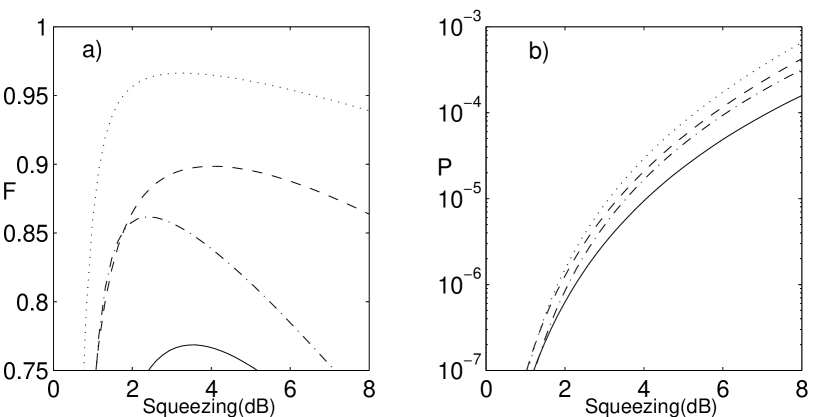
Figure 6: (a) Fidelity between the generated state and the target state and (b) probability of successful generation as a function of the squeezing $s_{\mathrm{in}}$ for the four target states (61) (solid line), (62) (dashed line), (63) (dot-dashed line), and (64) (dotted line), with $T=0.95$ and $\eta=0.25$.

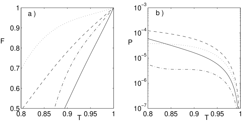
Figure 7: (a) Fidelity between the generated state and the target state and (b) probability of successful generation as a function of $T$ for the four target states (61)–(64). The curves are plotted considering the optimal squeezing $s_{\mathrm{in}}$ for each state, namely $3.54$ dB for state (61) (solid line), $4.02$ dB for state (62) (dashed line), $2.43$ dB for state (63) (dot-dashed line), and $3.24$ dB for state (64) (dotted line). The curves are plotted for $\eta=0.25$.

In order to illustrate our method, let us consider the following four squeezed superpositions of the Fock states $|0\rangle$, $|1\rangle$, and $|2\rangle$:

$$|\psi_{1}\rangle = S(s)|2\rangle,$$ (61)

$$|\psi_{2}\rangle = S(s)\frac{1}{\sqrt{2}}(|1\rangle+|2\rangle),$$ (62)

$$|\psi_{3}\rangle = S(s)\frac{1}{\sqrt{2}}(|0\rangle+|2\rangle),$$ (63)

$$|\psi_{4}\rangle = S(s)\frac{1}{\sqrt{3}}(|0\rangle+|1\rangle+|2\rangle),$$ (64)

We plot the behavior of the fidelity and probability of generation of the target states (61) – (64) as a function of the squeezing (Fig. 6), beam-splitter transmittance (Fig. 7), and photodetector efficiency (Fig. 8). As in the preceding section, we observe that the fidelity of the generation for any state gets arbitrarily close to one as $T$ approaches unity, as shown in Fig. 7. We also find that the fidelity is very robust against small detector efficiency $\eta$, as can be seen in Fig. 8. On the other hand, the preparation probability decreases with a growing $T$ and decreasing $\eta$, as predicted by the equation $P\propto(1-T)^{2}\eta^{2}$.

All these features are very similar to those found in the preceding section, where we considered only states generated with one photon subtraction. Let us now stress some new features. First, we note here the existence of a clear optimal squeezing, giving the maximum fidelity for each of the four studied states, see Fig. 6(a). Observing that the optimal squeezing has a higher value [from $2.4$ dB for state (63) to $4$ dB for state (62)] than those encountered in the case of one photon subtraction, we can expect an increasing value of the optimal squeezing for an increasing number of Fock states in the target superposition. It can be checked that the value of this optimal squeezing tends to zero when $T$ tends to 100%.

Another interesting fact is the existence of very different values of the optimum fidelity for different target states for a fixed $T=0.95$ and $\eta=0.25$, as shown in Fig. 6(a). For example, the squeezed two-photon state $S(s)|2\rangle$ is much more difficult to generate than the other three states (62)–(64). For the state $S(s)|2\rangle$, a transmittance of $T\gtrsim 0.99$ is necessary to reach a fidelity of $F\gtrsim 0.95$, resulting in a very low probability of generation. This would make the experimental generation of $S(s)|2\rangle$ with a good fidelity very challenging. In contrast, the squeezed balanced superposition state (64) can be generated with a high fidelity $F\gtrsim 0.90$ even with a transmittance $T\approx 0.90$.

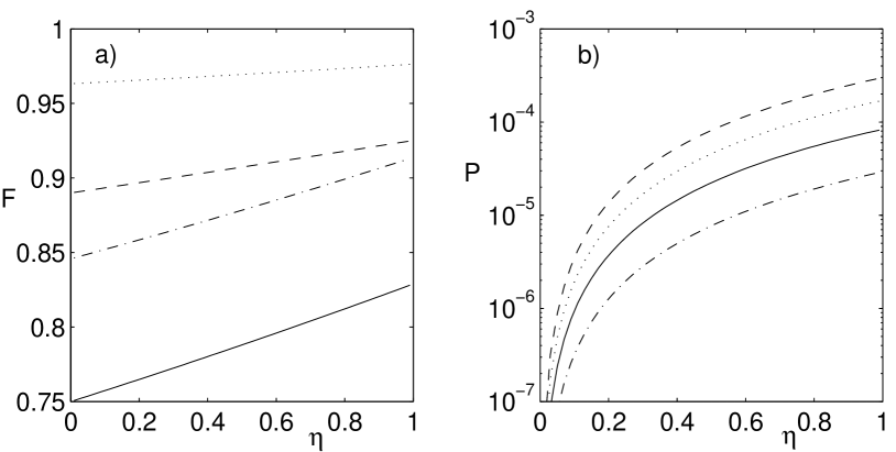
Figure 8: (a) Fidelity between the generated state and the target state and (b) probability of successful generation as a function of $\eta$ for the four target states (61)–(64). The curves are plotted considering the optimal squeezing $s_{\mathrm{in}}$ for each state, namely $3.54$ dB for state (61) (solid line), $4.02$ dB for state (62) (dashed line), $2.43$ dB for state (63) (dot-dashed line), and $3.24$ dB for state (64) (dotted line). The curves are plotted for $T=0.95$.

Another surprising fact arises when $\beta_{1}\neq\beta_{2}$. Then, the equations (60) give two distinct sets of $\alpha_{i}$’s generating the same arbitrary target state, the second set being obtained by making the exchange $\beta_{1}\leftrightarrow\beta_{2}$. Considering the pure-state description and $T\rightarrow 1$, the two alternative choices of displacements become strictly equivalent. In contrast, when considering the realistic model with $T<1$, these two solutions for the same target state do not have the exact same behavior. As we can see in Fig. 9(a), one of the two solutions is indeed more robust to decreasing $T$. However, the two solutions are rather similar as far as the probability of state generation is concerned, as shown in Fig. 9(b).

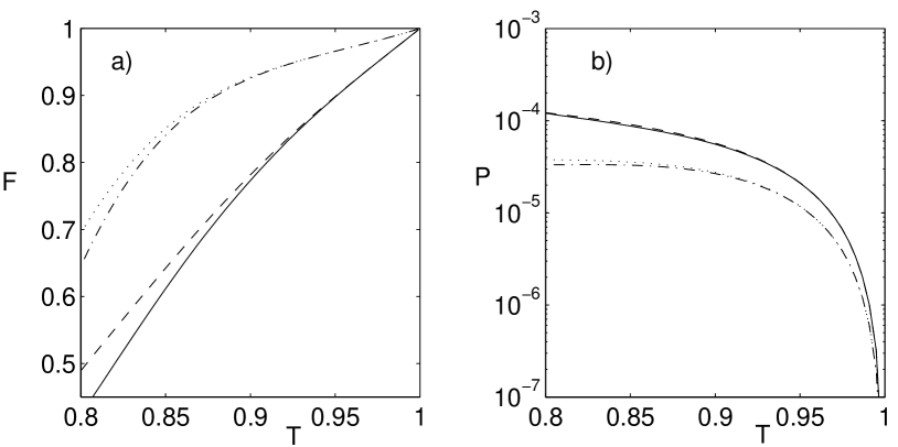
Figure 9: (a) Fidelity between the generated state and the target state and (b) probability of successful generation as a function of $T$ for the two target states (62) and (64). The curves correspond to the two alternatives choices of the displacements $\alpha_{1}$ and $\alpha_{2}$ when considering the optimal squeezing $s_{\mathrm{in}}$ for each state, namely $4.02$ dB for state (62) (dotted line, dot-dashed line), and $3.24$ dB for state (64) (dashed line, solid line). The curves are plotted for $\eta=0.25$.

IV Conclusions

In this paper, we have shown that an arbitrary single-mode state of light can be engineered starting from a squeezed vacuum and applying a sequence of displacements and single-photon subtractions. More precisely, the setup based on $N$ photon subtractions can be used to generate a squeezed superposition of the $N+1$ first Fock states. If this remaining squeezing is not desired, an extra squeezer can be added at the output of the setup in order to allow the generation of any (non-squeezed) superposition of the $N+1$ first Fock states.

We have shown that the desired target state can be successfully produced with arbitrarily high fidelity using a reasonably low squeezing ($\lesssim 3$dB) if the transmittance $T$ of the beam splitter used for photon subtraction is sufficiently close to unity (e.g. $T\simeq 95$%). This holds even when inefficient photodetectors with single-photon sensitivity but no single-photon resolution are employed, such as the commonly used avalanche photodiodes. We have studied the dependence of the achievable fidelity on the detection efficiency $\eta$, and have found that the scheme is very robust in the sense that the fidelity does almost not depend on $\eta$. Fidelities above $95$% could be reached even with $\eta$ of the order of a few percent if $T$ is high enough. However, low $\eta$ and high $T$ drastically reduce the preparation probability, so that a compromise has to be made when determining $T$.

Since our proposal does not require single-photon sources and can operate with low-efficiency photodetectors, its experimental implementation should be much easier than for the previous proposals, in particular the one based on repeated photon additions Dakna99 . The recent demonstration of single-photon subtraction from a single-mode squeezed vacuum Wenger04 provides a strong evidence for the practical feasibility of our scheme. In this experiment, a rather low overall detection efficiency ($\eta\approx 1$%) was reported, due to the spectral and spatial filtering of the beam measured by the photodetector. This is necessary because the OPA emits squeezed vacuum in several modes and the mode $A$ is selected in the experiment by the strong local oscillator pulse in balanced homodyne detector. Despite the filtering, the single-photon detector PD can be sometimes triggered by photons coming from other modes, so this would probably be the main source of imperfections in our scheme.

As a conclusion, we may reasonably assert that the generation of arbitrary squeezed superpositions of $|0\rangle$ and $|1\rangle$ should be experimentally achievable using our scheme with the present technology, while some improvement of the filtering and detection efficiency would probably be needed in order to extend the scheme to the preparation of squeezed superpositions of $|0\rangle$, $|1\rangle$, and $|2\rangle$.

- (1) B. Yurke, Phys. Rev. Lett. 56, 1515 (1986); B. Yurke, L. McCall, and J.R. Klauder, Phys. Rev. A 33, 4033 (1986).
- (2) M. Hillery and L. Mlodinow, Phys. Rev. A 48, 1548 (1993).
- (3) J.P. Dowling, Phys. Rev. A 57, 4736 (1998).
- (4) A.N. Boto, P. Kok, D.S. Abrams, S.L. Braunstein, C.P. Williams, and J.P. Dowling, Phys. Rev. Lett. 85, 2733 (2000).
- (5) G. Björk, L.L. Sánchez Soto, and J. Söderholm, Phys. Rev. Lett. 86, 4516 (2001).
- (6) D. Bouwmeester, A. Ekert, and A. Zeilinger, The Physics of Quantum Information (Springer, Berlin, 2000).
- (7) A. I. Lvovsky, H. Hansen, T. Aichele, O. Benson, J. Mlynek, and S. Schiller, Phys. Rev. Lett. 87, 050402 (2001).
- (8) A. Zavatta, S. Viciani, and M. Bellini, Phys. Rev. A 70, 053821 (2004).
- (9) J.W. Pan, D. Bouwmeester, M. Daniell, H. Weinfurter, and A. Zeilinger, Nature (London) 403, 515 (2000); J.-W. Pan, M. Daniell, S. Gasparoni, G. Weihs, and A. Zeilinger, Phys. Rev. Lett. 86, 4435 (2001).
- (10) P. Walther, K.J. Resch, T. Rudolph, E. Schenck, H. Weinfurter, V. Vedral, M. Aspelmeyer, and A. Zeilinger, Nature (London) 434, 169 (2005).
- (11) C.C. Gerry, A. Benmoussa, and R. A. Campos, Phys. Rev. A 66, 013804 (2002).
- (12) J. Fiurášek, Phys. Rev. A 65, 053818 (2002).
- (13) H. Lee, P. Kok, N.J. Cerf, and J.P. Dowling, Phys. Rev. A 65, 030101(R) (2002); P. Kok, H. Lee, and J.P. Dowling, Phys. Rev. A 65, 052104 (2002).
- (14) M. W. Mitchell, J. S. Lundeen, and A. M. Steinberg, Nature (London) 429, 161 (2004).
- (15) H.S. Eisenberg, J.F. Hodelin, G. Khoury, and D. Bouwmeester, Phys. Rev. Lett. 94, 090502 (2005).
- (16) M. Dakna, J. Clausen, L. Knöll, and D.-G. Welsch, Phys. Rev. A 59, 1658 (1999); Phys. Rev. A 60, 726 (1999).
- (17) J. Clausen, N. Hansen, L. Knoll, J. Mlynek, and D.G. Welsch, Applied Physics B-Lasers and Optics 72, 43 (2001).
- (18) C. J. Villas-Boas, Y. Guimaraes, M.H.Y. Moussa, and B. Baseia, Phys. Rev. A 63, 055801 (2001).
- (19) X.B. Zou, K. Pahlke, and W. Mathis, Phys. Lett. A 323, 329 (2004).
- (20) M. Dakna, T. Anhut, T. Opatrný, L. Knöll, and D.-G. Welsch, Phys. Rev. A 55, 3184 (1997).
- (21) A.P. Lund, H. Jeong, T.C. Ralph, and M. S. Kim, Phys. Rev. A 70, 020101(R) (2004).
- (22) H. Jeong and M. S. Kim, Phys. Rev. A 65, 042305 (2002).
- (23) T.C. Ralph, A. Gilchrist, G.J. Milburn, W.J. Munro, and S. Glancy, Phys. Rev. A 68, 042319 (2003).
- (24) K. J. Resch, J. S. Lundeen, and A. M. Steinberg, Phys. Rev. Lett. 88, 113601 (2002).
- (25) D. T. Pegg, L. S. Phillips, and S. M. Barnett, Phys. Rev. Lett. 81, 1604 (1998); M. Koniorczyk, Z. Kurucz, A. G bris, and J. Janszky, Phys. Rev. A 62, 013802 (2000).
- (26) S. A. Babichev, J. Ries, A. I. Lvovsky, Europhys. Lett. 64, 1 (2003)
- (27) S. A. Babichev, B. Brezger, and A. I. Lvovsky, Phys. Rev. Lett. 92, 047903 (2004)
- (28) T. Opatrný, G. Kurizki, and D.-G. Welsch, Phys. Rev. A 61, 032302 (2000); P.T. Cochrane, T.C. Ralph, and G.J. Milburn, Phys. Rev. A 65, 062306 (2002); S. Olivares, M.G.A. Paris, and R. Bonifacio, Phys. Rev. A 67, 032314 (2003).
- (29) M.S. Kim, E. Park, P.L. Knight, and H. Jeong, quant-ph/0409218.
- (30) J. Wenger, R. Tualle-Brouri, and Ph. Grangier, Phys. Rev. Lett. 92, 153601 (2004).
- (31) R. García-Patrón, J. Fiurášek, N.J. Cerf, J. Wenger, R. Tualle-Brouri, and Ph. Grangier, Phys. Rev. Lett. 93, 130409 (2004); R. García-Patrón, J. Fiurášek, and N.J. Cerf, Phys. Rev. A 71, 022105 (2005).
- (32) H. Nha and H. J. Carmichael, Phys. Rev. Lett. 93, 020401 (2004).
- (33) A. Kitagawa, M. Takeoka, K. Wakui, and M. Sasaki, quant-ph/0503049.
- (34) D.E. Browne, J. Eisert, S. Scheel, and M.B. Plenio, Phys. Rev. A 67, 062320 (2003); J. Eisert, D. Browne, S. Scheel, and M.B. Plenio, Annals of Physics (NY) 311, 431 (2004).
- (35) M.G.A. Paris, Phys. Lett. A 217, 78 (1996).
- (36) A. Furusawa et al., Science 282, 706 (1998).