Compatibility and Separability for Classical
and Quantum Entanglement

Abstract

We study the concepts of compatibility and separability and their implications for quantum and classical systems. These concepts are illustrated on a macroscopic model for the singlet state of a quantum system of two entangled spin 1/2 with a parameter reflecting indeterminism in the measurement procedure. By varying this parameter we describe situations from quantum, intermediate to classical and study which tests are compatible or separated. We prove that for classical deterministic systems the concepts of separability and compatibility coincide, but for quantum systems and intermediate systems these concepts are generally different.

1 Introduction

Entanglement is one of the main features of quantum mechanics. The most studied example of quantum entanglement is the one of the two spin 1/2 particles as presented by David Bohm [27]: more specifically in the situation where the joint quantum entity of the two spin 1/2 particles is in a singlet spin state. John Bell showed that quantum entanglement can be experimentally tested by means of a set of inequalities, meanwhile called Bell’s inequalities [26]. The ‘violation of Bell’s inequalities’ indicates the presence of quantum entanglement. In [3] an example of a situation consisting of macroscopic physical entities was proposed where Bell’s inequalities are violated. Later the example was elaborated to yield a violation with exactly the same value $2\sqrt{2}$ as the one that appears in the violation of Bell’s inequalities by the spins in the singlet spin state [10]. In the macroscopic example the considered entities are two macroscopic particles, and the entanglement is expressed by means of the presence of a rigid rod connecting the two particles. The rod represents the non-local effect that appears with the violation of Bell’s inequalities. In [20] it is shown that not only the singlet spin state, as considered in [3], but all entangled states of coupled spins can be represented by such a rod-like internal constraint. The quantum probability is obtained in the model because of the introduction of a hidden variable on the measurement apparatus in correspondence with the spin model that was developed in [6, 7].

The macroscopic model built in [3] violates Bell’s inequalities in a stronger way than the quantum spin example, indeed the violation value for the macroscopic model is 4 while for the quantum example it is $2\sqrt{2}$. We have proven in [14] that the quantum probability present in the case of the quantum spin example, and also in the macroscopic example of [3], decreases the violation of Bell’s inequalities. This is the reason that a purely classical non-local situation, like the one considered in [3], violates Bell’s inequalities in a stronger way, with maximum possible violation value $4$.

We know that two measurements of which each one is performed on one of the two spins of a quantum entangled spin couple are compatible measurements. Indeed, self-adjoint operators $H_{1}\otimes I_{2}$ and $I_{1}\otimes H_{2}$ representing these measurements commute, which means that the corresponding measurements are compatible. This means that a situation of quantum entanglement can produce correlations between compatible measurements that violate Bell’s inequalities. This is not possible for a situation of classical entanglements. Hence, if classical entanglement is present, at least some of the measurements on the left and on the right will be non-compatible measurements.

In the present article we investigate the aspect of compatibility and separability as defined in section 2 for situations of classical and quantum entanglement. We show in section 3 how increasing indeterminism, hence a change from classical entanglement to quantum-like entanglement, increases compatibility for measurements.

2 Quantum and Classical Entanglement

If we want to study compatibility and separability for macroscopic classical entities as well as for quantum entities, we need to introduce a definition that is general enough to capture all these situations. We do this in the framework of the Geneva-Brussels approach to operational quantum axiomatics, where the basic notions are the ones of tests, states and properties [29, 30, 1, 2, 4, 5, 31, 32]. Let us consider the situation of a physical entity $S$. The entity $S$ is described by a state space $\Sigma=\{p,q,\ldots\}$ and a set of tests $\mathcal{Q}=\{\alpha,\beta,\ldots\}$ which are defined by dichotomic experiments with outcomes ‘yes’ and ‘no’ (see [2, 5] for the terminology used). We denote $O(\alpha,p)\subseteq\left\{\hbox{`yes'},\hbox{`no'}\right\}$ the set of possible outcomes for the test $\alpha\in\mathcal{Q}$, the physical entity being in state $p\in\Sigma.$ Obviously the set of possible outcomes of the test $\alpha$ is $O\left(\alpha\right)=\cup_{p\in\Sigma}O(\alpha,p)=\left\{\hbox{`yes'},\hbox{`no'}\right\}.$ We consider the situation of two physical entities $S_{1}$ and $S_{2}$, with state spaces $\Sigma_{1}$ and $\Sigma_{2}$, and sets of tests $\mathcal{Q}_{{1}}$ and $\mathcal{Q}_{2}$. The two entities $S_{1}$ and $S_{2}$ form a compound entity $S$, with state space $\Sigma$, and set of tests $\mathcal{Q}$. Suppose that the compound entity $S$ is in state $p\in\Sigma$, and consider two tests $\alpha_{1}\in\mathcal{Q}_{1}$ and $\alpha_{2}\in\mathcal{Q}_{2}$. If tests $\alpha_{1}$ and $\alpha_{2}$ can be performed together on the compound entity $S$ we denote this joint test $E\left(\alpha_{1},\alpha_{2}\right)$. It will give rise to couples of outcomes $\left(x_{1},x_{2}\right)\in O\left(E\left(\alpha_{1},\alpha_{2}\right)\right)$, such that $x_{1}\in O(\alpha_{1})$ and $x_{2}\in O(\alpha_{2})$. Let us denote the probability that an experiment $\alpha$ yields an outcome $x_{\alpha}^{i}\in O\left(\alpha\right)$ for the entity $S$ being in the initial state $p\in\Sigma$ by $P(\alpha,x_{\alpha}^{i}\mid p).$

2.1 Compatibility

Suppose that one considers an experiment $E$ with four possible outcomes, let’s call them $x_{1},x_{2},x_{3}$ and $x_{4}$. Suppose now that we consider two sub-experiments of this experiment $E$, by identifying some of the outcomes. Hence $\alpha_{1}$ is the experiment that consists in performing $E$, and giving outcome ‘yes’ if we get $x_{1}$ or $x_{2}$ for $E$, and ‘no’ if we get $x_{3}$ or $x_{4}$ for $E$. The experiment $\alpha_{2}$ consists in performing $E$, where we give ‘yes’ if we get outcomes $x_{1}$ or $x_{3}$ and ‘no’ if we get outcomes $x_{2}$ or $x_{4}$. Since both subexperiments $\alpha_{1}$ and $\alpha_{2}$ consist in performing the big experiment $E$, we also perform $\alpha_{1}$ and $\alpha_{2}$ together whenever we perform $E$. Let us see how these two sub experiments are related towards each other. Suppose $x_{2}$ is a possible outcome for $E,$ hence ‘yes, no’ is a possible outcome for experiment $E.$ Then (by definition) ‘yes’ is possible for $\alpha_{1}$ and ‘no’ is possible for $\alpha_{2}$. This is also the case for the other ‘yes’ and ‘no’ combinations, which shows that $\alpha_{1}$ and $\alpha_{2}$ are compatible as defined in [1],[11]. Hence sub experiments of a big experiment defined in this straightforward way are always compatible experiments. Compatibility expresses the situation where the sub experiments behave as if they could be substituted by one big experiment, after identification of certain outcomes. In terms of probabilities of experiments, one can express the basis idea of compatibility, namely compatible experiments can be substituted by one big experiment such that they are recovered after identification of certain outcomes, by following conditions:

Definition 1 (Compatibility)

Tests $\alpha_{1}$ and $\alpha_{2}$ are ‘compatible’ tests with respect to a state $p\in\Sigma$ iff

$$P(\alpha_{1},\hbox{`yes'}\mid p) = P(E,x_{1}\mid p)+P(E,x_{2}\mid p)$$ (1)

$$P(\alpha_{1},\hbox{`no'}\mid p) = P(E,x_{3}\mid p)+P(E,x_{4}\mid p)$$ (2)

$$P(\alpha_{2},\hbox{`yes'}\mid p) = P(E,x_{1}\mid p)+P(E,x_{3}\mid p)$$ (3)

$$P(\alpha_{2},\hbox{`no'}\mid p) = P(E,x_{2}\mid p)+P(E,x_{4}\mid p)$$ (4)

In case of compatibility, when for example $P(E,x_{1}\mid p)$ is different from zero, hence (yes,yes) is a possible outcome, then $P(\alpha_{1},\hbox{`yes'}\mid p)$ and $P(\alpha_{2},\hbox{`yes'}\mid p)$ are different from zero (because probabilities cannot be smaller than zero), hence ‘yes’ is a possible outcome for $\alpha_{1}$ and ‘yes’ is a possible outcome for $\alpha_{2}$. Grasping the concept of compatibility in probabilistic terms instead of merely ‘yes-no’ statements as in [1],[11] allows for a more detailed and realistic classification of the experiments, in the sense that performing real experiments leads to probabilities rather than yes-no statements.

2.2 Separability

Suppose that we start now with two experiments $\alpha_{1}$ and $\alpha_{2}$, such that whatever one does with $\alpha_{1}$ does not influence what one does with $\alpha_{2}$ (the idea of separated of Einstein Podolsky Rosen, [28]), then, just from pure logic, follows that whenever $\alpha_{1}$ has a possible outcome ‘yes’ and for example $\alpha_{2}$ has a possible outcome ‘no’, then the joint experiments has as possible outcome the couple ‘yes, no’, because there is no influence. That is the basis of separability.

Definition 2 (Separability)

Two tests $\alpha_{1}$ and $\alpha_{2}$ are called ‘separated’ with respect to a state $p\in\Sigma$ iff

$$P(E,x_{1}\mid p) = P(\alpha_{1},\hbox{`yes'}\mid p)P(\alpha_{2},\hbox{`yes'}\mid p)$$ (5)

$$P(E,x_{2}\mid p) = P(\alpha_{1},\hbox{`yes'}\mid p)P(\alpha_{2},\hbox{`no'}\mid p)$$ (6)

$$P(E,x_{3}\mid p) = P(\alpha_{1},\hbox{`no'}\mid p)P(\alpha_{2},\hbox{`yes'}\mid p)$$ (7)

$$P(E,x_{4}\mid p) = P(\alpha_{1},\hbox{`no'}\mid p)P(\alpha_{2},\hbox{`no'}\mid p)$$ (8)

Definition 3 (Separated Tests)

Two tests $\alpha_{1}$ and $\alpha_{2}$ are ‘separated’ iff $\forall p\in\Sigma:\alpha_{1}$ and $\alpha_{2}$ are separated with respect to $p.$

This means that if $x_{1}\in O(\alpha_{1},p)$ and $x_{2}\in O(\alpha_{2},p)$ are possible outcomes for the tests $\alpha_{1}$ and $\alpha_{2}$ on the system $S$ in state $p$ then also the combined outcome $\left(x_{1},x_{2}\right)$ is a possible outcome for the joint test $E\left(\alpha_{1},\alpha_{2}\right)$. Suppose that for a specific state the experiment $E$ only has two possible outcomes, namely $x_{2}$ and $x_{3}$, then for this state the just constructed experiments $\alpha_{1}$ and $\alpha_{2}$ are not separated. Indeed if $E$ gives the outcome $x_{2}$ we get ‘yes’ for $\alpha_{1}$, and if $E$ gets the outcome $x_{3}$ we get ‘no’ for $\alpha_{1}$, which means that ‘yes’ and ‘no’ are possible outcomes for $\alpha_{1}$. In an analogous way it is easy to see that ‘yes’ and ‘no’ are possible outcomes for $\alpha_{2}$. But ‘yes, yes’ is not a possible outcome for $E$, which proves that $\alpha_{1}$ and $\alpha_{2}$ are not separated. In the example of ‘always compatible experiments’ it is clear that these experiments are not necessarily separated, since in this case they are ‘always’ executed together, which means that they are highly dependent, and not at all independent.

Let us notice that separability implies compatibility. Indeed, putting expressions (5-8) into (1-4) one can easily verify that compatibility holds. A necessary and also sufficient condition for two compatible experiments to be separated is the following:

$$P(E,x_{1}\mid p)P(E,x_{4}\mid p)=P(E,x_{2}\mid p)P(E,x_{3}\mid p)$$ (9)

Clearly this is a necessary condition for separability, and after some elementary calculations one can verify that it is also a sufficient condition for two compatible experiments to be separated.

2.3 Classicality

Definition 4 (Classicality)

A test $\alpha\in\mathcal{Q}$ is called a ‘classical test’ iff $\forall p\in\Sigma,\exists x\left(p\right)\in O\left(\alpha\right):$ $(\alpha,p)=\left\{x\left(p\right)\right\}.$

Hence for each state $p$ a classical test $\alpha$ yields a specific outcome $x\left(p\right)$ with certainty. Similarly a joint test $E\left(\alpha_{1},\alpha_{2}\right)$ is classical iff $\forall p\in\Sigma,\exists\left(x_{1},x_{2}\right)\left(p\right)\in O\left(E\left(\alpha_{1},\alpha_{2}\right)\right):$ $O(E\left(\alpha_{1},\alpha_{2}\right),p)=\left\{\left(x_{1},x_{2}\right)\left(p\right)\right\}.$

Definition 5 (Classical Entity)

An entity is called a classical entity iff all its tests are classical.

It is not possible to give an example of a classical entity with tests that are compatible but not separated. This is because for classical entities the two concepts are equivalent.

Theorem 1

If $\alpha_{1},\alpha_{2}$ are classical tests then $\alpha_{1}$ and $\alpha_{2}$ are compatible with respect to a state $p$ iff $\alpha_{1}$ and $\alpha_{2}$ are separated with respect to this state $p$.

Proof: Suppose $\alpha_{1}$ and $\alpha_{2}$ are classical tests that are compatible with respect to state $p$. Suppose ‘yes’ is a possible answer for $\alpha_{1}$ and ‘no’ is a possible answer for $\alpha_{2}$ in state $p$. Since both $\alpha_{1}$ and $\alpha_{2}$ are classical, these are the only respective outcomes for $\alpha_{1}$ and $\alpha_{2}$ such that $P(\alpha_{1},\hbox{`yes'}\mid p)=1=P(\alpha_{2},\hbox{`no'}\mid p).$ Consequently, $P(\alpha_{1},\hbox{`no'}\mid p)=P(\alpha_{2},\hbox{`yes'}\mid p)=0.$ Because of compatibility, $P(E,x_{1}\mid p)=P(E,x_{3}\mid p)=P(E,x_{4}\mid p)=0,$ such that $P(E,x_{2}\mid p)=1.$ Hence the requirement 9 is satisfied and tests $\alpha_{1}$ and $\alpha_{2}$ are separated tests. $\Box$

Hence for classical entities these concepts coincide, such that compatible classical tests are always separated. Also notice that classicality of the joint experiment follows from the compatibility of the classical subtests. That a joint test constructed from two classical subtests is not necessarily a classical test too, can be seen from following example. Let us consider a slightly modified version of the example given in [3, 14]. The entity consists of two vessels connected by a tube and contains 20 liters of transparent water. Tests $\alpha_{i}$ on the left, respectively right vessel are defined by taking a siphon and collecting water in a reference vessel. If we consider the test $\alpha_{i}$ defined as ‘can we take more than 10 liters of water from the vessel $i$’ then test $\alpha_{1}$ performed on the left vessel yields ‘yes’ with certainty. If on the other hand we would chose to perform the test $\alpha_{2}$ on the right vessel then we would obtain ‘yes’ with certainty. If we define the joint test $E\left(\alpha_{1},\alpha_{2}\right)$ by performing both tests $\alpha_{1}$ and $\alpha_{2}$ at the same time, we can never find the answer (‘yes’,‘yes’) showing that tests $\alpha_{1}$ and $\alpha_{2}$ are not compatible and hence not separated. An example of a joint test of two classical subtests which is not classical can be constructed as follows. Let us consider the test $\beta_{2}$ on the right vessel, defined as follows: ‘take a random amount of water (between 0,5 and 19,5 liter) out the right vessel with the fastest siphon in the universe and see whether the water is transparent or not’. Because of the initial assumption that the vessels are filled with transparent water, $\beta_{2}$ always yields the answer ‘yes’. Again, if we would perform test $\alpha_{1}$ we find the answer ‘yes’ with certainty such that $P(\alpha_{1},\hbox{`yes'}\mid p)=1=P(\beta_{2},\hbox{`yes'}\mid p).$ On the other hand, if the joint test $E\left(\alpha_{1},\beta_{2}\right)$ is performed by making both tests at the same time, then in some cases we obtain the outcome $\left(\hbox{`yes'},\hbox{`yes'}\right)$ in the case the random amount of water collected by test $\beta_{2}$ is less than 10 liters of water, and $\left(\hbox{`no'},\hbox{`yes'}\right)$ in the other case since test $\beta_{2}$ uses the fastest siphon and collects all the water it needs to check for transparency before test $\alpha_{1}$ is able to collect more than 10 liters of water. Hence the joint test is not classical, since $P(E,x_{1}\mid p)=P(E,x_{3}\mid p)=1/2.$ Also, tests $\alpha_{1}$ and $\beta_{2}$ are not compatible, since $P(E,x_{2}\mid p)=P(E,x_{4}\mid p)=0,$ such that $P(\alpha_{1},\hbox{`yes'}\mid p)=1\neq 1/2=P(E,x_{1}\mid p)+P(E,x_{2}\mid p).$ This example shows that compatibility of classical tests is a very powerful condition, since it not only implies separability of the two tests, but also classicality of the joint test.

For the example of the connected vessels of water it is clear that the considered tests cannot be separated because of the clear physical connection between the two vessels. For entangled quantum systems we encounter non-separated tests in a natural way (actually it is not possible to describe a compound system of two separated quantum systems within the formalism of quantum theory[1, 2, 4, 23, 24, 25]), but the origin of this quantum non-separability is still a matter of debate for physicists and philosophers alike. To shed more light on this issue, we discuss in the next section a macroscopic model of a compound system of two entangled spin 1/2 in the singlet state, in which tests are defined by a parameter reflecting randomness in the measurement such that we obtain a continuous transition from a quantum system to a classical system, and check what happens with separability and compatibility for these systems.

3 The Model

For the individual spin 1/2 entities of the coupled spin 1/2 entity we use a sphere model representation developed within the hidden measurement approach to quantum mechanics [6, 7, 8, 9, 13, 15], which is a generalization of the Poincaré or Bloch representation, such that also the measurements as well as a parameter for non-determinism are described [20].

In this model, a spin 1/2 entity is represented by a point particle on the surface of a 3-dimensional unit sphere, called Poincaré sphere, such that its state ${|\psi\rangle}=\left(\cos{\frac{\theta}{2}}e^{\frac{-i\phi}{2}},\sin{\frac{\theta}{2}}e^{\frac{i\phi}{2}}\right)$ is represented by the point $u(1,\theta,\phi)=(\sin\theta\cos\phi,\sin\theta\sin\phi,\cos\theta)$. All points of the Poincaré sphere represent states of the spin, such that points $u(1,\theta,\phi)$ on the surface correspond to pure states, while interior points $u(r,\theta,\phi)$ correspond to density states $D(r,\theta,\phi):$

$$D(r,\theta,\phi)={\frac{1}{2}}\left(\begin{array}[]{cc}1+r\cos\theta&r\sin\theta e^{-i\phi}\\ r\sin\theta e^{i\phi}&1-r\cos\theta\end{array}\right)$$ (10)

In this expression $D(1,\theta,\phi)={|\psi\rangle}{\langle\psi|}$ is the usual density state representation of a pure state, while $D(0,\theta,\phi)$ is the density matrix representing the center of the sphere.

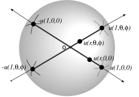
Figure 1: The Poincaré or Bloch sphere. Each point of the sphere represents a state of the spin 1/2. We have indicated 6 states explicitly, $u(1,\theta,\phi),u(r,\theta,\phi)$ and $-u(1,\theta,\phi)$, which are three states in the spin direction $(\theta,\phi)$, and $u(1,0,0),u(r,0,0)$ and $-u(1,0,0)$, which are three states in the spin direction $(0,0)$.

Next to this, the sphere model allows a representation of measurements by introducing an elastic band that is located along the measurement direction $u(\theta,\phi)$ (we omit the radius $1$ since the measurement direction is completely defined by angles $(\theta,\phi)$). We introduce a test $\alpha_{u(\theta,\phi)}^{\epsilon}$ that is the following. We put a piece of elastic of length $2\epsilon$ in the middle of the sphere and connect it with ‘unbreakable’ cords with the point $u(1,\theta,\phi)$ on the surface of the sphere and its diametrically opposite point $-u(1,\theta,\phi)$ (Fig. 1). Suppose that the spin is in a state represented by the point $u(r^{\prime},\theta^{\prime},\phi^{\prime})$. Once the elastic is placed, the point particle falls orthogonally from its place $u(r^{\prime},\theta^{\prime},\phi^{\prime})$ onto the elastic, and stays stuck to it in the point $u(1,\theta,\phi)\cdot u(r^{\prime},\theta^{\prime},\phi^{\prime})$. Then the piece of elastic breaks with uniform probability. If the elastic breaks in the interval $\left(-\epsilon,u(1,\theta,\phi)\cdot u(r^{\prime},\theta^{\prime},\phi^{\prime})\right)$ the elastic pulls the particle to the point $u(1,\theta,\phi)$ where it stays and the test $\alpha_{u(\theta,\phi)}^{\epsilon}$ yields answer ‘yes’. If on the other hand the elastic breaks in the interval $\left(u(1,\theta,\phi)\cdot u(r^{\prime},\theta^{\prime},\phi^{\prime}),\epsilon\right)$ the particle ends up in $-u(1,\theta,\phi)$ and the test $\alpha_{u(\theta,\phi)}^{\epsilon}$ yields the answer ‘no’.

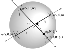
Figure 2: Between $-u(1,\theta,\phi)$ and $u(1,\theta,\phi)$ is a connection consisting of an elastic of length $2\epsilon$ around $0$, and an unbreakable cord for the rest. The point particle in $u(r^{\prime},\theta^{\prime},\phi^{\prime})$ falls orthogonally on this connection. Then the elastic breaks at random uniformly, and one of the two pieces of the connection drags the point particle to one of the two points $-u(1,\theta,\phi)$ or $u(1,\theta,\phi)$, respectively with probabilities that are the quantum spin 1/2 transition probabilities.

If the elastic breaks exactly in the point $u(1,\theta,\phi)\cdot u(r^{\prime},\theta^{\prime},\phi^{\prime})$ we make the hypothesis that the test $\alpha_{u(\theta,\phi)}^{\epsilon}$ yields the outcome ‘yes’. If $\epsilon=1,$ it can be proven that the sphere model reduces to a model for the spin measurements on a spin 1/2 particle, since the probabilities of the outcome ‘yes’ (respectively ‘no’) for the test $\alpha_{u(\theta,\phi)}^{1}$ coincide with the quantum probabilities for a spin measurement with a Stern-Gerlach apparatus along the $(\theta,\phi)$-direction (Fig. 2) [6, 7, 8, 9, 20]. Also, the corresponding state transitions are the same, namely a collapse from the initial state towards an eigenstate of the observed outcome. If $\epsilon=0$, the model reduces to a classical model: all tests $\alpha_{u(\theta,\phi)}^{0}$ are classical, in the sense of definition 4. Remark that in this classical limit ($\epsilon=0$) still a state transition occurs, but from the probabilistic point of view measurements behave classical (i.e. deterministic). For $0<\epsilon<1$ we find a situation in between quantum and classical [19, 21, 22, 17, 18]. Assuming uniform distribution of where the elastic breaks, probabilities are given by

$$P(\alpha_{u(\theta,\phi)}^{\epsilon},\hbox{`yes'}\mid p) = \frac{\epsilon+\cos\theta_{up}}{2\epsilon}$$

$$P(\alpha_{u(\theta,\phi)}^{\epsilon},\hbox{`no'}\mid p) = \frac{\epsilon-\cos\theta_{up}}{2\epsilon}$$

for $-\epsilon<\cos\theta_{up}<\epsilon,$ $P(\alpha_{u(\theta,\phi)}^{\epsilon},\hbox{`yes'}\mid p)=1$ for $\cos\theta_{up}\geq\epsilon,$ $P(\alpha_{u(\theta,\phi)}^{\epsilon},\hbox{`no'}\mid p)=1$ for $\cos\theta_{up}\leq-\epsilon.$

The connected vessels of water entity is already an example of a macroscopic system which violate Bell’s inequalities [1]. However, the expectation values it attains violate Bell’s inequalities more than possible for any quantum system of two entangled spin 1/2. In a way, this follows from the fact that the connected vessels of water entity behaves ‘too deterministic’: if we allow indeterminism in the tests one can obtain expectation values which still violate Bell’s inequalities but within the bounds of quantum probability [14]. In effect, in [9] a macroscopic system was considered which violates Bell’s inequalities in exactly the same way as a quantum system of two entangled spin 1/2 in the singlet state. The model consists of two sphere models, such that the point particles are connected by a rigid but extendable rod (Fig. 3). The singlet state is represented by the two point particles being in the center of the respective Poincaré sphere, which corresponds with a density state of the sphere model.

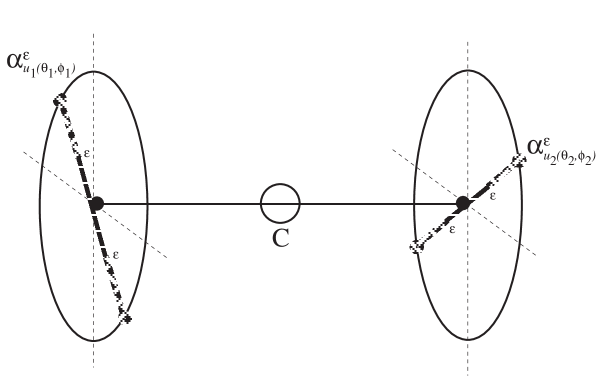
Figure 3: Symbolic representation of the singlet state in the model as two dots in the centers of their respective spheres. Also shown is the connecting rod and the measurement directions chosen at the left and right location

A joint test $E\left(\alpha_{1},\alpha_{2}\right)$ on the compound system is defined by performing first the test $\alpha_{1}$ and next the test $\alpha_{2}$ as follows. First let us consider the quantum case with $\epsilon=1$ and show that the model indeed is a model for the singlet state. When the first test $\alpha_{u(\theta_{1},\phi_{1})}^{1}$ is performed, one of the two possible outcomes occurs with probability 1/2 since the point particle is in the middle of the sphere and the elastic pulls the left point particle to the corresponding eigenstate. However, because of the rod between the two particles, the other particle which initially was in the center of the right sphere is drawn towards a point on the surface of the sphere, namely the point diametrically opposite to the eigenstate of the observed outcome of the first test. Only then the second test is performed on the point particle, following the same description as for a single sphere model. When the frequency of the coincidence counts is calculated it turns out to be in exact accordance with the quantum mechanical prediction for the spin measurements on a quantum system of two entangled spin 1/2 in the singlet state [10, 14]. Actually, because of symmetry in the initial singlet state it does not matter which test is performed first (left or right), since the results (i.e. probabilistic distribution over the set of outcomes and the corresponding final states) are the same.

There are two key ingredients of this model that seem particularly important in order to make it a model for the singlet state. First we have the rigid rod, which shows the non-separable wholeness of the singlet coincidence measurement (cfr. the role of the connecting tube between the vessels of water) and which reflects the role of non-locality in quantum theory. Secondly, we have the elastic that breaks which gives rise to the probabilistic nature (cfr. the role of the siphon in the vessels of water) of the outcomes which reflects the intrinsic indeterminism in quantum experiments. Together these features establish the meaning of the violation of Bell’s inequalities as the ‘non-existence of local realism’. Let us now explore the role of indeterminism for the concepts of separability and compatibility by introducing the parameter $\epsilon$ for the compound system in the singlet state in an analogous way as for a single spin 1/2 model (Fig 3).

We analyze for different values of the parameter $\epsilon$ which tests are compatible or separated. Consider the case $\epsilon=1$, which means that our model becomes a quantum model for two coupled spin 1/2 in the singlet spin state. Consider the tests $\alpha_{u_{1}(\theta_{1},\phi_{1})}^{1}$ and $\alpha_{u_{2}(\theta_{2},\phi_{2})}^{1}$ for $\theta_{1}=\theta_{2}$ and $\phi_{1}=\phi_{2}$, hence the case of two aligned spin directions.

Then the coupled sphere models are compatible but not separable: while for each test $\alpha_{1}$ and $\alpha_{2}$ the result ‘yes’ or ‘no’ is possible (with probability 1/2), the joint test $E\left(\alpha_{1},\alpha_{2}\right)$ only has possible outcomes (‘yes’,‘no’) or (‘no’,‘yes’) for the compound system in the singlet state, each with probability 1/2. Hence $P(E,x_{2}\mid p)=P(E,x_{3}\mid p)=1/2$ and the two tests are compatible but not separable: $P(E,x_{1}\mid p)=0\neq 1/4=P(\alpha_{1},\hbox{`yes'}\mid p)P(\alpha_{2},\hbox{`yes'}\mid p).$ The same situation occurs if we consider the tests $\alpha_{u_{1}(\theta_{1},\phi_{1})}^{1}$ and $\alpha_{u_{2}(\theta_{2},\phi_{2})}^{1}$, with $\theta_{1}=\pi-\theta_{2}$ and $\phi_{1}=\pi+\phi_{2}$ (i.e. $u_{1}$ and $u_{2}$ are opposite directions): for both tests the result ‘yes’ or ‘no’ are possible outcomes (with probability 1/2), while the joint test only has possible outcomes (‘yes’,‘yes’) or (‘no’,‘no’) for the compound system in the singlet state. Hence also these tests are compatible but not separable. We remark that if we consider tests $\alpha_{u_{1}(\theta_{1},\phi_{1})}^{1}$ and $\alpha_{u_{2}(\theta_{2},\phi_{2})}^{1}$ along different measurement directions $(\theta_{1},\phi_{1})$ and $(\theta_{2},\phi_{2})$, we find that these tests are always compatible:

$$P(E,x_{1}\mid p) = \frac{1}{2}\sin^{2}\left(\frac{\theta_{uv}}{2}\right)$$

$$P(E,x_{2}\mid p) = \frac{1}{2}\cos^{2}\left(\frac{\theta_{uv}}{2}\right)$$

$$P(E,x_{3}\mid p) = \frac{1}{2}\cos^{2}\left(\frac{\theta_{uv}}{2}\right)$$

$$P(E,x_{4}\mid p) = \frac{1}{2}\sin^{2}\left(\frac{\theta_{uv}}{2}\right)$$

but that they are only separable if $\theta_{u_{1}u_{2}}=\frac{\pi}{2}$ in which case the second measurement yields the same probability distribution after performing the first experiment as for a single measurement, and it is as if the subtests could be performed independently of each other.

Let us now consider the case $0<\epsilon<1$ and determine which tests are compatible, respectively separable. Let us first notice that for the system prepared in the singlet state we have $P\left(\alpha_{i},\hbox{`yes'}\right)=P\left(\alpha_{i},\hbox{`no'}\right)=1/2.$ Following the description of the compound tests $E\left(\alpha_{u_{1}(\theta_{1},\phi_{1})}^{\epsilon},\alpha_{u_{2}(\theta_{2},\phi_{2})}^{\epsilon}\right)$ for the system prepared in the singlet state, the point particle in the second sphere will be pulled by means of the rod to the point $-u_{1}(1,\theta_{1},\phi_{1})$ on the sphere in the event of an answer ‘yes’ in the first test, and to the point $u_{1}(1,\theta_{1},\phi_{1})$ in the event of an outcome ‘no’. Hence if in the first subtest of the joint experiment $E\left(\alpha_{u_{1}(\theta_{1},\phi_{1})}^{\epsilon},\alpha_{u_{2}(\theta_{2},\phi_{2})}^{\epsilon}\right)$ the outcome ‘yes’ was found, then outcome ‘yes’ occurs in the second measurement with probability

$$P(\alpha_{2},\hbox{`yes'}\mid-u_{1}(1,\theta_{1},\phi_{1}))=\frac{\epsilon+\cos\theta_{-u_{1}u_{2}}}{2\epsilon}=\frac{\epsilon-\cos\theta_{u_{1}u_{2}}}{2\epsilon}$$ (11)

if $-\epsilon<\cos\theta_{u_{1}u_{2}}<\epsilon$, such that $P(E,x_{1}\mid p)=\frac{1}{2}\frac{\epsilon-\cos\theta_{u_{1}u_{2}}}{2\epsilon}.$ If $\cos\theta_{u_{1}u_{2}}\geq\epsilon$ we obtain $P(E,x_{1}\mid p)=0,$ and if $\cos\theta_{u_{1}u_{2}}\leq-\epsilon$ then $P(E,x_{1}\mid p)=1/2.$ Similarly, we find for $-\epsilon\leq\cos\theta_{u_{1}u_{2}}\leq\epsilon$

$$P(E,x_{1}\mid p) = \frac{1}{2}\frac{\epsilon-\cos\theta_{u_{1}u_{2}}}{2\epsilon}$$

$$P(E,x_{2}\mid p) = \frac{1}{2}\frac{\epsilon+\cos\theta_{u_{1}u_{2}}}{2\epsilon}$$

$$P(E,x_{3}\mid p) = \frac{1}{2}\frac{\epsilon+\cos\theta_{u_{1}u_{2}}}{2\epsilon}$$

$$P(E,x_{4}\mid p) = \frac{1}{2}\frac{\epsilon-\cos\theta_{u_{1}u_{2}}}{2\epsilon}$$

Clearly, the two experiments $\alpha_{u_{1}(\theta_{1},\phi_{1})}^{\epsilon}$ and $\alpha_{u_{2}(\theta_{2},\phi_{2})}^{\epsilon}$ are always compatible but only separated if $\cos\theta_{u_{1}u_{2}}=0,$ i.e. $\theta_{u_{1}u_{2}}=\frac{\pi}{2}.$

Finally, let us see what happens in the classical situation $\epsilon=0$ for $\alpha_{u_{1}(\theta_{1},\phi_{1})}^{0},\alpha_{u_{2}(\theta_{2},\phi_{2})}^{0}$. The first test $\alpha_{u_{1}(\theta_{1},\phi_{1})}^{0}$ is deterministic since it yields answer ‘yes’ with certainty, such that the second particle is pulled towards the state $-u_{1}(1,\theta_{1},\phi_{1})$. If $u_{2}(1,\theta_{2},\phi_{2})\cdot u_{1}(1,\theta_{1},\phi_{1})>0$ the second test $\alpha_{u_{2}(\theta_{2},\phi_{2})}^{0}$ yields answer ‘no’ with certainty. If $u_{2}(1,\theta_{2},\phi_{2})\cdot u_{1}(1,\theta_{1},\phi_{1})\leq 0$ the second test will yield the outcome ‘yes’ with certainty. Hence depending on the angle between the measurement directions $u_{2}(1,\theta_{2},\phi_{2})$ and $u_{1}(1,\theta_{1},\phi_{1})$ we obtain that the set of possible outcomes for the joint test $E\left(\alpha_{u_{1}(\theta_{1},\phi_{1})}^{0},\alpha_{u_{2}(\theta_{2},\phi_{2})}^{0}\right)=\left\{\left(\hbox{`yes'},\hbox{`no'}\right)\right\}$ if $u_{2}(1,\theta_{2},\phi_{2})\cdot u_{1}(1,\theta_{1},\phi_{1})>0$ and $E\left(\alpha_{u_{1}(\theta_{1},\phi_{1})}^{0},\alpha_{u_{2}(\theta_{2},\phi_{2})}^{0}\right)=\left\{\left(\hbox{`yes'},\hbox{`yes'}\right)\right\}$ if $u_{2}(1,\theta_{2},\phi_{2})\cdot u_{1}(1,\theta_{1},\phi_{1})\leq 0.$ Since for $\epsilon=0$ both test $\alpha_{u_{1}(\theta_{1},\phi_{1})}^{0}$ and $\alpha_{u_{2}(\theta_{2},\phi_{2})}^{0}$ yield positive outcome with certainty: $P\left(\alpha_{u_{1}(\theta_{1},\phi_{1})}^{0},\hbox{`yes'}\right)=1=P\left(\alpha_{u_{2}(\theta_{2},\phi_{2})}^{0},\hbox{`yes'}\right)$, we can conclude that for $u_{2}(1,\theta_{2},\phi_{2})\cdot u_{1}(1,\theta_{1},\phi_{1})\leq 0$ the two tests are compatible, and from theorem 1 (or simple verification) follows that they are also separable. For $u_{2}(1,\theta_{2},\phi_{2})\cdot u_{1}(1,\theta_{1},\phi_{1})>0$ we have $P(E,x_{2}\mid p)=1=P(\alpha_{u_{1}(\theta_{1},\phi_{1})}^{0},\hbox{`yes'}\mid p)=P(\alpha_{u_{2}(\theta_{2},\phi_{2})}^{0},\hbox{`yes'}\mid p)$. Hence tests along these directions are neither compatible nor separable, which is in agreement with theorem 1 which states that for classical tests the concepts of compatibility and separability coincide.

4 Conclusions

We have studied a macroscopic model for the singlet state of a quantum system of two spin 1/2 consisting of two sphere models connected by a rigid but extendable rod. By considering a parameter representing indeterminism in the measurement procedure, we have described a continuous transition from a quantum to a classical system and shown which tests are compatible or separable. We have proven that for classical, i.e. deterministic, systems the concepts of separability and compatibility coincide, and that the joint test of two compatible classical subtests is classical. As an illustration we considered an example of a nonclassical joint test of two classical but noncompatible subtests. For the compound system in the quantum limit tests along non orthogonal measurement directions are always compatible but not separable. Therefore, these tests and a fortiori the subsystems are not separated, which is in agreement with previous results stating that separated quantum entities cannot be described in quantum theory [1, 2, 4, 23, 24, 25]. For intermediate values of the parameter we found that all tests are compatible, but they are only separable if $\theta_{u_{1}u_{2}}=\frac{\pi}{2}.$ In the classical limit $\epsilon=0$ tests $\alpha_{u_{1}(\theta_{1},\phi_{1})}^{0}$ and $\alpha_{u_{2}(\theta_{2},\phi_{2})}^{0}$ are compatible and therefore also separable if $u_{2}(1,\theta_{2},\phi_{2})\cdot u_{1}(1,\theta_{1},\phi_{1})\leq 0$. In these cases, the two subsystems behave as if they are really separated and their is no rigid rod connecting the two point particles. If $u_{2}(1,\theta_{2},\phi_{2})\cdot u_{1}(1,\theta_{1},\phi_{1})>0$ tests $\alpha_{u_{1}(\theta_{1},\phi_{1})}^{0}$ and $\alpha_{u_{2}(\theta_{2},\phi_{2})}^{0}$ are not compatible and in accordance with theorem 1 also not separated, the role of the rigid rod cannot be neglected.

References

- [1] Aerts, D., 1981, The One and the Many: Towards a Unification of the Quantum and Classical Description of One and Many Physical Entities, Doctoral dissertation, Brussels Free University.
- [2] Aerts, D., 1982, Description of many physical entities without the paradoxes encountered in quantum mechanics, Foundations of Physics, 12, 1131-1170.
- [3] Aerts, D., 1982, Example of a macroscopical situation that violates Bell inequalities, Lettere al Nuovo Cimento, 34, 107-111.
- [4] Aerts, D., 1983, The description of one and many physical systems. In C. Gruber (Ed.), Foundations of Quantum Mechanics (63-148), Lausanne, AVCP.
- [5] Aerts, D., 1983, Classical theories and nonclassical theories as a special case of a more general theory, Journal of Mathematical Physics, 24, 2441-2453.
- [6] Aerts, D., 1985, A possible explanation for the probabilities of quantum mechanics and a macroscopical situation that violates Bell inequalities. In P. Mittelstaedt and E. W. Stachow (Eds.), Recent Developments in Quantum Logic, Grundlagen der Exacten Naturwissenschaften, vol.6, Wissenschaftverlag (235-251), Mannheim, Bibliographisches Institut.
- [7] Aerts, D., 1986, A possible explanation for the probabilities of quantum mechanics, Journal of Mathematical Physics, 27, 202-210.
- [8] Aerts, D., 1987, The origin of the non-classical character of the quantum probability model. In A. Blanquiere, S. Diner and G. Lochak (Eds.), Information, Complexity, and Control in Quantum Physics (77-100), New York, Springer.
- [9] Aerts, D., 1991, A macroscopical classical laboratory situation with only macroscopical classical entities giving rise to a quantum mechanical probability model. In L. Accardi (Ed.), Quantum Probability and Related Topics, Volume VI (75-85), Singapore, World Scientific.
- [10] Aerts, D., 1991, A mechanistic classical laboratory situation violating the Bell inequalities with , exactly ‘in the same way’ as its violations by the EPR tests, Helvetica Physica Acta, 64, 1-24.
- [11] Aerts, D., 1994, Quantum structures, separated physical entities and probability, Foundations of Physics, 24, 1227-1259.
- [12] Aerts, D., 1999, Foundations of quantum physics: a general realistic and operational approach, International Journal of Theoretical Physics, 38, 289-358.
- [13] Aerts, D., Aerts, S., 1997, The hidden measurement formalism: quantum mechanics as a consequence of fluctuations on the measurement. In M. Ferrero and A. van der Merwe (Eds.), New Developments on Fundamental Problems in Quantum Physics, Dordrecht, Kluwer Academic.
- [14] Aerts, D., Aerts, S., Broekaert, J. and Gabora, L. 2000. The violation of Bell inequalities in the macroworld. Foundations of Physics, 30, pp. 1387-1414. Archive reference and link: http://uk.arxiv.org/abs/quant-ph/0007044.
- [15] Aerts, D., Aerts, S., Coecke, B., D’Hooghe, B., Durt, T. and Valckenborgh, F, 1997, A model with varying fluctuations in the measurement context. In M. Ferrero and A. van der Merwe (Eds.), New Developments on Fundamental Problems in Quantum Physics, Dordrecht, Kluwer Academic.
- [16] Aerts, D., Aerts, S., Coecke, B. and Valckenborgh, F., 1995, The meaning of the violation of Bell Inequalities: nonlocal correlation or quantum behavior?, preprint, Brussels Free University.
- [17] Aerts, D., Coecke, B., Durt, T. and Valckenborgh, F., 1997, Quantum, classical and intermediate I: a model on the poincare sphere, Tatra Mountains Mathematical Publications, 10, 225.
- [18] Aerts, D., Coecke, B., Durt, T. and Valckenborgh, F., 1997, Quantum, classical and intermediate II: the vanishing vector space structure, Tatra Mountains Mathematical Publications, 10, 241.
- [19] Aerts, D., Durt, T., Van Bogaert, B., 1993, A physical example of quantum fuzzy sets and the classical limit, Tatra Mountains Mathematical Publications, 1, 5-15.
- [20] Aerts, D., D’Hondt, E. and D’Hooghe, B. (in press). A geometrical representation of entanglement as internal constraint. International Journal of Theoretical Physics. Archive reference and link: http://uk.arxiv.org/abs/quant-ph/0211094.
- [21] Aerts, D., Durt, T., 1994, Quantum, classical and intermediate, an illustrative example, Foundations of Physics, 24, 1353-1369.
- [22] Aerts, D., Durt, T., 1994, Quantum, classical and intermediate: a measurement model. In K. V. Laurikainen, C. Montonen and K. Sunnaborg (Eds.), Symposium on the Foundations of Modern Physics, Gives Sur Yvettes, France, Editions Frontieres.
- [23] Aerts, D. and Valckenborgh, F., 2002, The linearity of quantum mechanics at stake: the description of separated quantum entities. In D. Aerts, M. Czachor and T. Durt (Eds.), Probing the Structure of Quantum Mechanics: Nonlinearity, Nonlocality, Probability and Axiomatics (pp. 20-46), Singapore, World Scientific. Archive reference and link: http://uk.arxiv.org/abs/quant-ph/0205161.
- [24] Aerts, D. and Valckenborgh, F., 2002, Linearity and compound physical systems: the case of two separated spin 1/2 entities. In D. Aerts, M. Czachor and T. Durt (Eds.), Probing the Structure of Quantum Mechanics: Nonlinearity, Nonlocality, Probability and Axiomatics (pp. 47-70), Singapore, World Scientific. Archive reference and link: http://uk.arxiv.org/abs/quant-ph/0205166.
- [25] Aerts, D. and Valckenborgh, F., 2004, Failure of standard quantum mechanics for the description of compound quantum entities. International Journal of Theoretical Physics, 43, 251-264.
- [26] Bell, J. 1964, On the Einstein-Podolsky-Rosen paradox, Physics, 1, 195.
- [27] Bohm, D. 1989, Quantum Theory. New York: Dover Publications.
- [28] Einstein, A. Podolsky, B. and Rosen, N., 1935, Can quantum-mechanical description of reality be considered complete? Physical Review 47, 777-780.
- [29] Piron, C., 1964, Axiomatique quantique, Helvetica Physica Acta, 37, 439.
- [30] Piron, C., 1976, Foundations of Quantum Physics, Reading, Mass., W. A. Benjamin.
- [31] Piron, C., 1989, Recent Developments in Quantum Mechanics, Helvetica Physica Acta, 62, 82.
- [32] Piron, C., 1990, Mècanique Quantique: Bases et Applications,, Press Polytechnique de Lausanne.