Dissipative quantum chaos: transition from wave packet collapse to explosion

Abstract

Using the quantum trajectories approach we study the quantum dynamics of a dissipative chaotic system described by the Zaslavsky map. For strong dissipation the quantum wave function in the phase space collapses onto a compact packet which follows classical chaotic dynamics and whose area is proportional to the Planck constant. At weak dissipation the exponential instability of quantum dynamics on the Ehrenfest time scale dominates and leads to wave packet explosion. The transition from collapse to explosion takes place when the dissipation time scale exceeds the Ehrenfest time. For integrable nonlinear dynamics the explosion practically disappears leaving place to collapse.

Technological progress leads to the investigation of physical phenomena at smaller and smaller scales, where both quantum and dissipative effects play a very important role. At present, general theoretical concepts for the description of quantum dissipative systems are well developed and established weissbook ; ingold . A major tool is the master equation, that governs the evolution of the density matrix lindblad . For the simplest dynamics this equation can be solved exactly. However, for complex nonlinear systems analytical solution is absent and even numerical simulations become very difficult. Indeed, for a system whose Hilbert space has dimension $N$, one has to store and evolve a density matrix of size $N\times N$. In spite of these limitations, numerical simulations of the master equation allowed to perform the first studies of the quantum dynamics of classically chaotic dissipative systems showing a quantum strange attractor graham .

Quantum trajectories are a very convenient tool to simulate dissipative systems schack ; brun . Instead of direct solution of the master equation, quantum trajectories allow us to store only a stochastically evolving state vector of size $N$. By averaging over many runs we get the same probabilities (within statistical errors) as the ones obtained through the density matrix directly. Besides their practical convenience, quantum trajectories also provide a good illustration of individual experimental runs dalibard . Indeed, modern experiments often enable us to address a single quantum system evolving under the unavoidable influence of the environment.

It is known that for linear systems dissipation leads to wave packet localization linear . Numerical results as well as theoretical arguments indicated that localization can occur also in nonlinear systems schack2 ; percival . On the other side, in absence of dissipation it is known that the instability of classical dynamics leads to exponentially fast spreading of the quantum wave packet on the logarithmically short Ehrenfest time scale $t_{E}\sim|\ln\hbar|/\lambda$ berman ; chirikov81 . Here $\lambda$ denotes the Lyapunov exponent which gives the rate of exponential instability of classical chaotic motion, and $\hbar$ is the dimensionless effective Planck constant of the system. In this paper we show that for the dissipative quantum chaos there exist two regimes: one with the wave packet explosion (delocalization) induced by chaotic dynamics and another with the wave packet collapse (localization) caused by dissipation. We argue that the transition (or crossover) from collapse to explosion takes place when the dissipation time $1/\gamma$ becomes larger than the Ehrenfest time $t_{E}$ ($\gamma$ is the dissipation rate).

We investigate the quantum evolution of a kicked system subjected to a dissipative friction force. Assuming the Markov approximation, we can write a master equation in the Lindblad form lindblad :

$$\dot{\hat{\rho}}=-i[\hat{H},\hat{\rho}]-\frac{1}{2}\sum_{\mu}\{\hat{L}_{\mu}^{{\dagger}}\hat{L}_{\mu},\hat{\rho}\}+\sum_{\mu}\hat{L}_{\mu}\hat{\rho}\hat{L}_{\mu}^{{\dagger}},$$ (1)

where $\hat{\rho}$ is the density operator, { , } denotes the anticommutator, $\hat{L}_{\mu}$ are the Lindblad operators, which model the effects of the environment, and $\hat{H}$ is the Hamiltonian of the system. We consider a kicked system, described by the Hamiltonian

$$\hat{H}=\frac{\hat{n}^{2}}{2}+k\cos\,(\hat{x})\sum_{m=-\infty}^{+\infty}\delta(\tau-mT),$$ (2)

where $T$ is the kicking period and the operators $\hat{x}$ and $\hat{n}=-i(d/dx)$ come from quantizing the classical variables $x\in[0,2\pi[$ and $n\in(-\infty,+\infty)$. This Hamiltonian corresponds to the kicked rotator izrailev , a paradigmatic model in the fields of nonlinear dynamics and quantum chaos. This model is also on the focus of experimental investigations with cold atoms in optical lattices raizen . We assume that dissipation is described by the lowering operators

$$\begin{array}[]{l}\hat{L}_{1}=g\sum_{n}\sqrt{n+1}\;|n\rangle\,\langle n+1|,\\ \hat{L}_{2}=g\sum_{n}\sqrt{n+1}\;|-n\rangle\,\langle-n-1|,\end{array}$$ (3)

with $n=0,1,...$ eigenvalues of the operator $\hat{n}$. At the classical limit, the evolution of the system in one period is described by the Zaslavsky map zaslavsky

$$\left\{\begin{array}[]{l}n_{t+1}=(1-\gamma)n_{t}+k\sin x_{t},\\ x_{t+1}=x_{t}+Tn_{t+1},\end{array}\right.$$ (4)

where the discrete time $t$ is measured in number of kicks and $1-\gamma=\exp(-g^{2})$. This map describes a friction force proportional to velocity. We have $0\leq\gamma\leq 1$; the limiting cases $\gamma=0$ and $\gamma=1$ correspond to Hamiltonian evolution and overdamped case, respectively. Introducing the rescaled momentum variable $p=Tn$, we can see that the classical dynamics depends only on the parameters $K=kT$ and $\gamma$. Since $[\hat{x},\hat{p}]=[\hat{x},T\hat{n}]=iT$, the effective Planck constant is $\hbar=T$. The classical limit corresponds to $\hbar\to 0$, while keeping $K=\hbar k=const$.

The first two terms of Eq. (1) can be regarded as the evolution governed by an effective non-Hermitian Hamiltonian, $\hat{H}_{\rm eff}=\hat{H}_{s}+i\hat{W}$, with $\hat{W}=-1/2\sum_{\mu}\hat{L}_{\mu}^{{\dagger}}\hat{L}_{\mu}$. In turn, the last term is responsible for the so-called quantum jumps. Taking an initial state $|\phi(\tau_{0})\rangle$, the jump probabilities $dp_{\mu}$ in an infinitesimal time $d\tau$ are defined by $dp_{\mu}\!=\!\langle\phi(\tau_{0})|\hat{L}_{\mu}^{{\dagger}}\hat{L}_{\mu}|\phi(\tau_{0})\rangle d\tau,$ and the new states after the jumps by $|\phi_{\mu}\rangle=\hat{L}_{\mu}|\phi(\tau_{0})\rangle/||{L}_{\mu}|\phi(\tau_{0})\rangle||$. With probability $dp_{\mu}$ a jump occurs and the system is left in the state $|\phi_{\mu}\rangle$. With probability $1-\sum_{\mu}dp_{\mu}$ there are no jumps and the system evolves according to the effective Hamiltonian $\hat{H}_{\rm eff}$. In this case we end up with the state $|\phi_{0}\rangle={(\openone-iH_{\rm eff}dt/\hbar)|\phi(t_{0})\rangle}/{\sqrt{1-\sum_{k}dp_{k}}}$. We note that the normalization is included also in this case because the evolution governed by $\hat{H}_{\rm eff}$ is non-Hermitian. To simulate numerically the above described jump picture we use the so-called Monte Carlo wave function approach dalibard . The changing state of a single open quantum system is represented directly by a stochastically evolving quantum wave function, as for a single run of a laboratory experiment. We say that a single evolution is a quantum trajectory.

We focus first on the chaotic regime for the kicked rotator dynamics. Therefore, we consider $K=7$, corresponding to a positive Lyapunov exponent $\lambda\approx\ln(K/2)=1.25$. The localization-delocalization transition is clearly illustrated in the two top panels of Fig. 1. They show the Husimi function Husimi corresponding to a single quantum trajectory evolution, computed after $t=300$ kicks. In both cases the initial wave packet is a Gaussian state with equal uncertainties $\Delta x=\Delta p=\sqrt{\hbar/2}$. We can see that for strong dissipation ($\gamma=0.5$) the wave function of a single quantum trajectory at $t=300$ is localized in the phase space (top left panel in Fig. 1). In contrast, the case of weak dissipation ($\gamma=0.01$, top right) is characterized by wave packet delocalization. Since for strong dissipation the wave packet is localized in phase space, it makes sense to draw a quantum Poincaré section by printing the expectation values $\langle x\rangle$ and $\langle p\rangle$ at each map step. The quantum Poincaré section is shown in Fig. 1 (bottom left) and is characterized by the appearance of a strange attractor. A very similar strange attractor is obtained also from the classical Poincaré section corresponding to the Zaslavsky map (4) (see Fig. 1 bottom right). We also note that the Husimi function obtained in the case of weak dissipation exhibits a spreading of the quantum wave packet over the strange attractor. Also in the strongly dissipative regime the localized wave packet is stretched along the direction of the attractor.

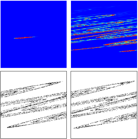
Figure 1: (color online) Top: Husimi functions in phase space for a single quantum trajectory taken after $t=300$ kicks, at $K=7$, $\hbar=0.012$, $\gamma=0.5$ (left) and $\gamma=0.01$ (right). Here the coordinates $x$ (horizontal axis) and $p$ (vertical axis) vary in the intervals: $0\leq x<2\pi$, $-25\leq p\leq 25$ (left) and $-100\leq p\leq 50$ (right); the width of the $p$-interval is the same in both cases for comparison purposes. The initial Gaussian wave packet is located at $(\langle x\rangle,\langle p\rangle)=(5\pi/4,0)$. The color is proportional to density: blue for zero and red for maximum. Bottom: quantum Poincaré section (left), obtained from average quantum $x,p$ values for the case of top left panel and its classical counterpart (right). In these panels $0\leq x<2\pi$ and $-15\leq p\leq 15$.

A further confirmation of the good agreement between the classical and quantum dissipative evolutions is obtained by computing the function $f\equiv\langle p\rangle_{t+1}-(1-\gamma)\langle p\rangle_{t}$ noted . From the classical map (4) we expect $f(x)=K\sin x$. The comparison between $f(\langle x\rangle)$ and the function $f(x)$, shown in Fig. 2, indicates that the Zaslavsky map provides a good description of the quantum wave packet motion. Indeed the points $f(\langle x\rangle)$ are concentrated around the curve $f(x)$, with dispersion proportional to $\sqrt{\hbar}$ (see Fig. 4 below). Therefore a quantum trajectory exhibits the same important features of a classical trajectory, including the exponential instability, with rate given by the classical Lyapunov exponent. A significant difference between quantum and classical trajectories is the presence of quantum noise noise . Therefore, a more precise identification can be done between quantum evolution and noisy classical evolution, the noise amplitude being $\Delta x\sim\Delta p\propto\sqrt{\hbar}$. It is interesting to note that the chaotic behavior of classical systems can be reproduced also by non-dissipative continuously measured quantum systems habib ; milburn ; deutsch .

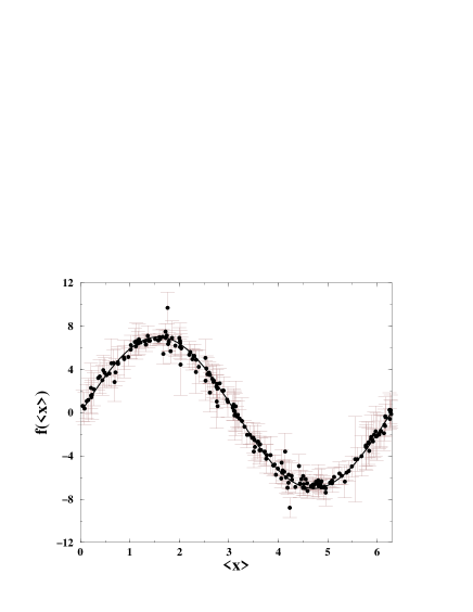
Figure 2: Comparison between $f(\langle x\rangle)$ computed from the quantum dynamics (circles) and the kick function $f(x)=K\sin x$ (solid curve). Parameter values and initial conditions are as in Fig. 1 (left top and bottom panels). Error bars represent the quantum uncertainty in $f(\langle x\rangle)$.

The wave packet dispersion is measured by $\sigma_{t}=\sqrt{(\Delta x)_{t}^{2}+(\Delta p)_{t}^{2}}$. This quantity is evaluated, for weak and strong dissipation, in Fig. 3 (left panel), using the same parameter values and initial conditions as in Fig. 1. In both cases there are strong fluctuations, which we smooth down by computing the cumulative average $\overline{\sigma}_{t}\equiv\frac{1}{t}\sum_{j=1}^{t}\sigma_{j}$. The convergence of the time averaged quantity $\overline{\sigma}_{t}$ to a limiting value is clear. It is also evident that the wave packet spreading is much stronger at weak than at strong dissipation. We would like to stress that the same limiting value of the average dispersion $\overline{\sigma}$ is obtained for any quantum trajectory, independently of the initial condition. This is demonstrated in the right panel of Fig. 3, where we compare $\overline{\sigma}_{t}$ for two completely different initial conditions: a Gaussian wave packet and an eigenstate of the operator $\hat{x}$, that is, $|x\rangle=|x_{0}\rangle$. In the latter case there is a complete delocalization along $p$ (limited only by the size of the basis considered in our numerical simulations) and dissipation leads to the collapse of the wave packet, which eventually becomes localized in phase space.

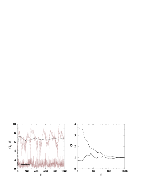
Figure 3: Left: Dispersion $\sigma$ (fluctuating curves) and cumulative average $\overline{\sigma}$ (smooth curves) as a function of the number of kicks $t$, for the cases considered in Fig. 1, with $\gamma=0.01$ (dashed curves) and $\gamma=0.5$ (full curves). Right: $\overline{\sigma}$ versus time $t$ at $\gamma=0.5$, starting from an initial Gaussian wave packet (full curve, also shown in the left panel) and a coordinate eigenstate $|x\rangle=|x_{0}\rangle$, with $x_{0}=\pi$ (dashed curve).

The average dispersion $\overline{\sigma}$ of the wave packet as a function on the dissipation strength $\gamma$ is shown in Fig. 4, for a few values of the effective Planck constant $\hbar$, with $0.012\leq\hbar\leq 0.33$. The localization-delocalization transition can be seen for all $\hbar$ values. In Fig. 4 inset we consider the scaled dispersion $\overline{\sigma}_{s}\equiv\overline{\sigma}/\sqrt{\hbar}$. At strong dissipation all curves collapse, while at weak dissipation the scaling $\overline{\sigma}\propto\sqrt{\hbar}$ is not fulfilled. Our numerical results can be explained as follows. Due to the exponential instability of chaotic dynamics the wave packet spreads exponentially and for times shorter than the Ehrenfest time we have $\sigma_{t}\sim\sqrt{\hbar}\exp(\lambda t)$. The dissipation localizes the wave packet on a time scale of the order of $1/\gamma$. Therefore, for $1/\gamma\ll t_{E}$, we obtain $\overline{\sigma}\sim\sqrt{\hbar}\exp(\lambda/\gamma)\ll 1$. In contrast, for $1/\gamma>t_{E}$ the chaotic wave packet explosion dominates over dissipation and we have complete delocalization over the angle variable. In addition, in this case, the wave packet spreads algebraically due to diffusion for $t>t_{E}$. For $t\gg t_{E}$ we have $\sigma_{t}\sim\sqrt{D(K)t}$, $D(K)\approx K^{2}/2$ being the diffusion coefficient. This regime continues up to the dissipation time $1/\gamma$, so that $\overline{\sigma}\sim\sqrt{D(K)/\gamma}$. According to the above argument, the transition from collapse to explosion, which we wish to call Ehrenfest explosion, takes place at

$$t_{E}\sim|\ln\hbar|/\lambda\sim 1/\gamma\;.$$ (5)

Our numerical data at moderate values of $\hbar>0.01$ indicate a smooth transition (crossover). However, we cannot exclude from our data that in the limit $\hbar\rightarrow 0$ the transition becomes sharp. Since the dependence on $\hbar$ is only logarithmic it is difficult to check numerically the above relation. However, it is compatible with our data obtained for $\hbar>0.01$. First of all, in the localized regime $\gamma t_{E}>1$ the scaling law $\overline{\sigma}\propto\sqrt{\hbar}$ is satisfied. Moreover, it is satisfied down to smaller and smaller $\gamma$ values when $\hbar$ is reduced. Therefore, even for infinitesimal dissipation strengths the quantum wave packet is eventually localized when $\hbar\to 0$: we have $\lim_{\hbar\to 0}\overline{\sigma}=0$. In contrast, in the Hamiltonian case ($\gamma=0$) $\lim_{\hbar\to 0}\overline{\sigma}=\infty$. This result underlines the importance of a (dissipative) environment in driving the quantum to classical transition: only for open quantum systems the classical concept of trajectory is meaningful for arbitrarily long times. On the contrary, for Hamiltonian systems a description based on wave packet trajectories is possible only up to the Ehrenfest time scale.

We would like to emphasize the role played by chaotic motion. For this purpose, in Fig. 4 we also show $\overline{\sigma}$ as a function of $\gamma$ in the integrable regime at $K=0.7$, for $\hbar=0.012$. In this case the wave packet dispersion is much smaller than in the chaotic regime: the Ehrenfest time scale is algebraic and not logarithmic in $\hbar$. Thus, a much weaker dissipation is sufficient to localize the wave function in the case of integrable dynamics. This can be clearly seen from our numerical data shown in Fig. 4.

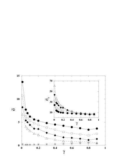
Figure 4: Average dispersion $\overline{\sigma}$ as a function of $\gamma$, for $K=7$, $\hbar=0.33$ (circles), $0.11$ (squares), $0.036$ (diamonds) and $0.012$ (triangles). Stars show the same quantity for the integrable case $K=0.7$, at $\hbar=0.012$. Inset: scaled dispersion $\overline{\sigma}_{s}=\overline{\sigma}/\sqrt{\hbar}$ versus $\gamma$, with same meaning of symbols as in the main figure.

Finally, we would like to point out that the transition described here could be observed by means of Bose-Einstein condensates in optical lattices. A first experimental implementation of the kicked rotator model using a Bose-Einstein condensate has been recently reported newzeland . Dissipative cooling techniques are possible in these systems. Moreover, images of atomic clouds can be taken, thus measuring their dispersion. Also the measured condensate positions should give a clean kick function (like in Fig. 2) in the case of collapse and random scattered points in the case of explosion. Such experiments would give important information not only on the interplay between chaos and dissipation but also on the stability of the condensate raizen2 under the joint effects of chaotic dynamics and dissipation.

This work was supported in part by EU (IST-FET-EDIQIP).

References

- (1) U. Weiss, Quantum dissipative systems (2nd Edition), World Scientific, Singapore (1999).
- (2) T. Dittrich, P. Hänggi, G.-L. Ingold, B. Kramer, G. Schön, and W. Zwerger, Quantum transport and dissipation (Wiley, Weinheim, 1998).
- (3) G. Lindblad, Commun. Math. Phys. 48, 119 (1976); V. Gorini, A. Kossakowski, and E.C.G. Sudarshan, J. Math. Phys. 17, 821 (1976).
- (4) T. Dittrich and R. Graham, Annals of Physics 200, 363 (1990).
- (5) T.A. Brun, I.C. Percival, and R. Schack, J. Phys. A 29, 2077 (1996).
- (6) T.A. Brun, Am. J. Phys. 70, 719 (2002).
- (7) J. Dalibard, Y. Castin, and K. Mølmer, Phys. Rev. Lett. 68, 580 (1992).
- (8) J. Halliwell and A. Zoupas, Phys. Rev. D 52, 7294 (1995).
- (9) R. Schack, T.A. Brun, and I.C. Percival, J. Phys. A 28, 5401 (1995).
- (10) I.C. Percival, J. Phys. A 27, 1003 (1994).
- (11) G.P. Berman and G.M. Zaslavsky, Physica A 91, 450 (1978).
- (12) B.V. Chirikov, F.M. Izrailev, and D.L. Shepelyansky, Sov. Scinet. Rev. (Gordon & Bridge), 2C, 209 (1981); Physica D 33, 77 (1988); D.L. Shepelyansky, Dokl. Akd. Nauk (SSSR) 256, 586 (1981) [Sov. Phys. Dokl. 26, 80 (1981).
- (13) F.M. Izrailev, Phys. Rep. 196, 299 (1990).
- (14) F.L. Moore, J.C. Robinson, C.F. Bharucha, B. Sundaram, and M.G. Raizen, Phys. Rev. Lett. 75, 4598 (1995).
- (15) R.Z. Sagdeev, D.A. Usikov, and G.M. Zaslavsky, Nonlinear Physics, Harwood Acad. Pub., NY (1988).
- (16) The Husimi function is obtained from smoothing the Wigner function on the scale of the Planck constant, see e.g. S.-J. Chang and K.-J. Shi, Phys. Rev. A 34, 7 (1986).
- (17) We note that can be determined from average positions.
- (18) Note that this difference is hardly visible in the Poincaré sections of Fig. 1, drawn on a scale much larger than the Planck cell.
- (19) T. Bhattacharya, S. Habib, and K. Jacobs, Phys. Rev. Lett. 85, 4852 (2000).
- (20) A.J. Scott and G.J. Milburn, Phys. Rev. A 63, 042101 (2001)
- (21) S. Ghose, P. Alsing, I. Deutsch, T. Bhattacharya, and S. Habib, Phys. Rev. A 69, 052116 (2004).
- (22) G.J. Duffy, S. Parkins, T. Müller, M. Sadgrove, R. Leonhardt, and A.C. Wilson, Phys. Rev. E 70, 056206 (2004).
- (23) C. Zhang, J. Liu, M.G. Raizen, and Q. Niu, Phys. Rev. Lett. 92, 054101 (2004).