The Bell Theorem as a Special Case of a Theorem of Bass

Abstract

The theorem of Bell states that certain results of quantum mechanics violate inequalities that are valid for objective local random variables. We show that the inequalities of Bell are special cases of theorems found ten years earlier by Bass and stated in full generality by Vorob’ev. This fact implies precise necessary and sufficient mathematical conditions for the validity of the Bell inequalities. We show that these precise conditions differ significantly from the definition of objective local variable spaces and as an application that the Bell inequalities may be violated even for objective local random variables.

1 Introduction

Einstein-Podolsky-Rosen (EPR) [1] suggested that quantum mechanics was incomplete and that hidden variables may be needed for completion. This was the subject of an extensive debate with Bohr [2] who denied the existence of such hidden variables using his well known reasoning that is at the basis of the Copenhagen interpretation of quantum mechanics. A mathematical non-existence proof for these hidden variables was presented by von Neumann within the framework of quantum mechanics. Bell [3], however, showed that von Neumann’s proof assumed the simultaneous measurability of certain quantities that could not possibly be simultaneously measured. Subsequently Bell himself presented a non-existence proof [4] in form of inequalities that are derived by using more complex assumptions that did not necessarily include simultaneous measurability.

The inequalities of Bell [4] are derived by the use of probability theory, in essence by the use of very elementary facts about random variables within the framework pioneered by Kolmogorov. The derivation of the inequalities does not involve physics or quantum mechanics, yet the inequalities have assumed an important role for the foundations of quantum mechanics. This role is a consequence of the assumptions for the random variables (and other possible variables) that are used to derive the Bell inequalities. It is commonly believed that these assumptions are needed and moreover are equivalent to the basic postulates of an “objective local” parameter space [5]. These postulates or conditions encompass Einstein-locality and the existence of elements of reality in the sense of Mach that co-determine the outcome of measurements. The fact that some results of quantum mechanics violate the Bell inequalities has therefore led to the belief that no objective local parameter space can exist that explains all the results of quantum mechanics.

Subsequent to these discussions experiments were proposed [6], [7] and later realized [8] that confirmed the theoretical result of quantum mechanics. This seemed to leave only difficult options for theoretical physics such as (i) to deny that the microscopic entities of physics have objective reality (non-existence of objective local parameters) or (ii) to assert that an influence can be propagated faster than the speed of light [9]. Additional options involving the validity of counterfactual reasoning have also been suggested and will be discussed below.

We show in this paper that because of the historical sequence of events, viz. the development of Bell’s theory before the performance of the actual experiments, some very important facts of probability theory have not been considered and/or misinterpreted . These facts are connected with the concept of a probability space that is important to link probability theory and mathematical statistics to the evaluation of actual experiments. We reconsider here these concepts and show that violations of the Bell inequalities have a purely mathematical reason, in particular that the Bell inequalities represent a special case of theorems given earlier by Bass [10], Vorob’ev [11], [12] and Schell [13]. These theorems permit us to deduce that, for all the possible Bell inequalities to be valid, it is a necessary and sufficient condition that the random variables involved in their proof are defined on one common probability space. Beyond this we show that the requirement of the use of one common probability space does not follow from the requirements of objective local spaces and vice versa. In fact, we show that there exist objective local random variables that can not be defined on a common probability space and therefore do not need to obey the Bell inequalities. As mentioned, Bell has dismissed von Neumann’s proof that assumed from the start the simultaneous measurability of the observables that correspond to our random variables and that can not be measured simultaneously. Our contribution here is that we also dismiss non-existence proofs of certain systems of random variables that need to be defined on one common probability space when it is clear from the outset that these systems of random variables can not be defined on any common probability space. We believe that our results give additional options of explanation for Aspect-type experiments without violating relativity or denying objective reality.

2 Mathematical model of a singlet spin state EPR experiment

As outlined above, probability theory provides a probability space and random variables and the link to the statistical treatment of the data from an actual experiment. Bell [4] considered an experimental situation advocated by Bohm and Aharonov [6], and by Bohm and Hiley [7]. This proposal was transformed into an actual experiment by Aspect et al. [8] including the suggestion of Bell and others that a rapid change of the settings needed to be implemented to accomplish a delayed choice situation [8]. We develop now an idealized experiment and a probability model for this actual experiment by Aspect et al within the framework of Kolmogorov. We note that our procedure also applies to other related experiments.

We first recall the concepts of a (discrete) probability space and of a random variable defined on it. As Feller states [14]“If we want to speak about experiments or observations in a theoretical way and without ambiguity, we first must agree on the simple events representing the thinkable outcomes; they define the idealized experiment…… By definition every indecomposable result of the (idealized) experiment is represented by one, and only one, sample point. The aggregate of all sample points will be called the sample space.” In our case of the idealized EPR experiment, the simple event can be chosen, for example, as the event of sending out one (and only one) correlated pair. With this event we associate an element $\omega$. In order to avoid mathematical technicalities that are not needed for the purpose of our paper we assume that the sample space $\Omega$ is at most countable. Each simple event $\omega\in\Omega$ is assigned the probability $P(\omega)$ that $\omega$ occurs. $P$ is a set function, defined for all subsets of $\Omega$, that satisfies the usual axioms, such as countable additivity and it assigns to $\Omega$ the value $P(\Omega)=1$. The pair $(\Omega,P)$ is called a probability space. A random variable is a real-valued function on $\Omega$, but if needed it also can assume values in high-dimensional space.

We now turn to the specifics of an idealized EPR-experiment. A correlated spin pair in the singlet state is sent out from a source in opposite directions toward measurement stations. These stations are characterized by certain randomly and rapidly switched settings which we denote by three dimensional unit vectors ${\bf a},{\bf b},{\bf c},...$. The measurements in the stations are mathematically represented by random variables $A=\pm 1,B=\pm 1,C=\pm 1,...$ that may in turn be functions of other random variables e.g. a source parameter $\Lambda$ that characterizes all the properties of the particles sent out from the source. $A$ indicates that the measurements that correspond to the outcomes of random variable $A$ have been performed using the setting $\bf a$ and similarly for $B$ and $C$.

We perform three categories of experiments, each with a different pair of setting vectors. The first category is characterized by the vectors $\bf a$ in station $S_{1}$ and $\bf b$ in station $S_{2}$. According to our notational convention we denote the pair of measurements $(A,B)$ and the joint probability density of $A$ and $B$ by $f_{1}$. Thus $f_{1}$ is given by

$$f_{1}(+1,+1)=P(A=+1,B=+1)\text{ , }f_{1}(-1,+1)=P(A=-1,B=+1)$$

$$f_{1}(+1,-1)=P(A=+1,B=+-1)\text{ , }f_{1}(-1,-1)=P(A=-1,B=-1)$$ (1)

The second category of experiments will be characterized by the vectors $\bf a$ in $S_{1}$ and $\bf c$ in $S_{2}$ with the resulting pair of measurements $(A,C)$ having density $f_{2}$, and the third category by the vectors $\bf b$ in $S_{1}$ and $\bf c$ in $S_{2}$ resulting in a pair of measurements $(B,C)$ with density $f_{3}$.

The measurement outcomes on both sides need to be completely random and $\pm 1$ with equal probability, i.e. all three distributions have identical marginals. This is dictated by the rules of quantum mechanics and verified by experiment. From this it follows that the $f_{i},i=1,2,3$ have the center of gravity for their point masses at the origin $(0,0)$ and

$$f_{i}(+1,-1)+f_{i}(+1,+1)=\frac{1}{2}=f_{i}(+1,+1)+f_{i}(-1,+1)\text{ for }i=1,2,3$$ (2)

The idealized mathematical model with exactly the properties described above and used within the framework of Kolmogorov is the basis for all our further considerations and we call it the Ma-EPR model.

3 Ma-EPR and the theorems of Bass and Vorob’ev

We start with an example that illustrates the theorems of Bass [10] and Vorob’ev [12] for the special case of the Ma-EPR model. The essential point of these theorems is that, in general, it is not possible to find three random variables $A,B$ and $C$, defined on a common probability space such that the three pairs $(A,B)$, $(A,C)$, and $(B,C)$ of random variables have their joint densities equal to $f_{1},f_{2}$ and $f_{3}$, respectively. Hence the notation that is commonly used and that we also introduced in section 2 above is misleading in the sense that it suggests there exist three random variables $A,B$ and $C$ that can reproduce the joint densities $f_{1}$, $f_{2}$ and $f_{3}$, when in fact they can not. Here is a modification of an example of Vorob’ev [12].

	$(+1,+1)$	$(+1,-1)$	$(-1,+1)$	$(-1,-1)$
$f_{1}(.,.)$	$3/8$	$1/8$	$1/8$	$3/8$
$f_{2}(.,.)$	$3/8$	$1/8$	$1/8$	$3/8$
$f_{3}(.,.)$	$1/8$	$3/8$	$3/8$	$1/8$

Table 1: Vorob’ev-type example [12].

Clearly Eq(2) holds. Suppose now that three such random variables $A,B$ and $C$ exist and are defined on one common probability space. Then the first two rows would imply that $P(A=B)=\frac{3}{4}=P(A=C)$, and so $P(B\neq C)\leq\frac{1}{2}$ , contradicting the fact that according to the third row $P(B=C)=\frac{1}{4}$. Another easy way to see that three such random variables cannot be defined on a common probability space follows from the fact that, for instance, it is not possible to assign a probability to the event $(A=1,B=1,C=1)$. According to the first entry of the third row this probability could not exceed $\frac{1}{8}$. Subtracting this value from the first entry of the first row we obtain that P(A = 1, B = 1, C = -1) would have to be at least $\frac{1}{4}$. But this is in conflict with the second entry of the second row. The reason for this phenomenon is that, picturesquely speaking, the three pair distributions form a closed loop. The joint densities of $(A,B)$ and of $(A,C)$ already contain some information about the joint density of $(B,C)$. Hence we do not have complete freedom to choose the latter one. This was shown for three general pair distributions by Jean Bass [10] and independently by Schell [13] who also investigated the connection with certain problems in economics. Vorob’ev [11], [12] established necessary and sufficient conditions that any complex of distributions must possess so that these distributions can be realized as marginal distributions of a set of random variables defined on a common probability space.

	$(+1,+1)$	$(+1,-1)$	$(-1,+1)$	$(-1,-1)$
$f_{1}(.,.)$	${\frac{1}{4}}(1+\sigma_{1})$	${\frac{1}{4}}(1-\sigma_{1})$	${\frac{1}{4}}(1-\sigma_{1})$	${\frac{1}{4}}(1+\sigma_{1})$
$f_{2}(.,.)$	${\frac{1}{4}}(1+\sigma_{2})$	${\frac{1}{4}}(1-\sigma_{2})$	${\frac{1}{4}}(1-\sigma_{2})$	${\frac{1}{4}}(1+\sigma_{2})$
$f_{3}(.,.)$	${\frac{1}{4}}(1+\sigma_{3})$	${\frac{1}{4}}(1-\sigma_{3})$	${\frac{1}{4}}(1-\sigma_{3})$	${\frac{1}{4}}(1+\sigma_{3})$

Table 2: Pair densities in terms of covariances

It is easy to show that under the assumption of Eq(2) the joint pair densities can be expressed in terms of the covariances $\sigma_{i},i=1,2,3$ defined by these pair densities. The pair densities are then given by Table 2 (see also the Lemma below). Note that the covariances $\sigma_{i}$ do not exceed $1$ in absolute value. Suppose now that there exist three random variables $A,B,C$ defined on one common probability space that reproduce the densities $f_{1},f_{2},f_{3}$ in Table 2. Then $\sigma_{1}=E(AB)$, $\sigma_{2}=E(AC)$, and $\sigma_{3}=E(BC)$ where $E$ denotes the expectation value. Expressing the entries of Table 2 in terms of the eight unknown probabilities $P(A=\pm 1,B=\pm 1,C=\pm 1)$ will result in a system of twelve linear equations in these eight unknowns that can be solved in an elementary way. In particular, solving this system shows that these eight probabilities can be expressed in terms of the three covariances $\sigma_{i},i=1,2,3$. It turns out that five of these twelve linear equations are redundant. Thus this system has infinitely many solutions. Taking into account that the solutions of this system represent probabilities $P\geq 0$ we obtain in a straightforward way that the following four inequalities are necessary and sufficient conditions for the solvability of the consistency problem for the three pair distributions given in Table 2:

$$1+\sigma_{1}+\sigma_{2}+\sigma_{3}\geq 0$$ (3)

$$1+\sigma_{1}-\sigma_{2}-\sigma_{3}\geq 0$$ (4)

$$1-\sigma_{1}+\sigma_{2}-\sigma_{3}\geq 0$$ (5)

$$1-\sigma_{1}-\sigma_{2}+\sigma_{3}\geq 0$$ (6)

Of course, the necessity part of this conclusion can be shown directly and trivially by modifying the standard proofs of the Bell inequality along the lines shown in [4].

4 Bell’s inequalities as a special case of Bass-Vorob’ev

Replacing the covariances $\sigma$ by the corresponding expectation values, one obtains from Eqs.(4-5):

$$E(AB)-E(AC)\leq 1-E(BC)$$ (7)

and

$$-E(AB)+E(AC)\leq 1-E(BC)$$ (8)

Eqs.(7) and (8) give

$$|E(AB)-E(AC)|\leq 1-E(BC)$$ (9)

This is, of course, one of the celebrated Bell inequalities. Five more can be obtained in analogous fashion from Eqs.(3-6) giving a total of 6 (4 choose 2). These can also be obtained by cyclic permutation in Eq.(9) and replacing both minus signs by plus signs.

Bass [10] proved that for three general pair distributions the consistency problem can be solved if and only if the triple $(\sigma_{1},\sigma_{2},\sigma_{3})$ considered as a point in $R^{3}$ belongs to a certain domain. In the special case we have been considering this domain reduces to the tetrahedron defined by the inequalities of Eqs.(3-6). We shall call it the covariance tetrahedron. It is diplayed in Fig. 1.

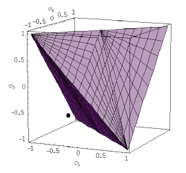
Figure 1: Covariance Tetrahedron. The solid point represents a choice of values that violates the Bell inequalities.

We formulate now our findings for the Ma-EPR experiment as a theorem. We first collect a few facts of section 3 above in form of a lemma.

Lemma: Let $f$ be a density supported on the four vertices $(\pm 1,\pm 1)$ of a square. Suppose that

$$f(+1,+1)+f(+1,-1)=f(+1,+1)+f(-1,+1)=\frac{1}{2}$$ (10)

Then

$$\sum xf(x,y)=\sum yf(x,y)=0$$ (11)

where the sums are extended over the four points $(x,y)=(\pm 1,\pm 1)$. Conversely, if $f$ satisfies Eq.(11) then $f$ also satisfies Eq.(10).

Set

$$\sigma:=\sum xyf(x,y)$$ (12)

with the same proviso for the sum. Then $f$ can be expressed in terms of $\sigma$ by the equations

$$f(+1,+1)=f(-1,-1)={\frac{1}{4}}(1+\sigma)$$ (13)

$$f(-1,+1)=f(+1,-1)={\frac{1}{4}}(1-\sigma)$$ (14)

Theorem1: Let $f_{1},f_{2},f_{3}$ be three probability densities satisfying the hypotheses of the Lemma with corresponding covariances $\sigma_{1},\sigma_{2},\sigma_{3}$. Then the following statements are equivalent

1. The point $(\sigma_{1},\sigma_{2},\sigma_{3})\in R^{3}$ satisfies the system of inequalities Eqs.(3-6) and therefore belongs to the covariance tetrahedron.

2. The point $(\sigma_{1},\sigma_{2},\sigma_{3})$ satisfies the following six Bell-type inequalities

   $$|\sigma_{1}-\sigma_{2}|\leq 1-\sigma_{3}\text{ , }|\sigma_{1}+\sigma_{2}|\leq 1+\sigma_{3}$$

   $$|\sigma_{1}-\sigma_{3}|\leq 1-\sigma_{2}\text{ , }|\sigma_{1}+\sigma_{3}|\leq 1+\sigma_{2}$$

   $$|\sigma_{2}-\sigma_{3}|\leq 1-\sigma_{1}\text{ , }|\sigma_{2}+\sigma_{3}|\leq 1+\sigma_{1}$$ (15)

3. There exist three random variables $A,B,C$ defined on a single common probability space with the following properties. The joint probability densities of $(A,B),(A,C)$ and $(B,C)$ are $f_{1},f_{2}$ and $f_{3}$ respectively. In particular, the expectation values equal

   $$E(A)=E(B)=E(C)=0$$ (16)

   the covariances equal

   $$E(AB)=\sigma_{1}\text{ , }E(AC)=\sigma_{2}\text{ , }E(BC)=\sigma_{3}$$ (17)

   Using Eqs.(15) and (17) one obtains the six Bell inequalities for the expectation values $E(AB),E(AC),E(BC)$.

Proofs: The proof of the Lemma is straightforward. The proof that conditions (I) and (II) of Theorem1 are equivalent can be done by inspection. The proof that (III) implies (II) or the six Bell inequalities obtained from Eq.(15) and Eq.(17) can be carried out by a simple modification of the standard proof of the Bell inequalities [4]. Finally, the proof that (I) implies (III) was outlined at the end of section 3.

We have shown therefore the following. The inequalities of Bell are a special case of the theorems of Bass and Vorob’ev for the Ma-EPR experiment. If the 6 Bell inequalities are valid then it is possible to find three random variables $A,B$ and $C$, defined on one common probability space that reproduce the three joint pair densities $f_{i}$ of Table 2 and their covariances $\sigma_{1}=E(AB),\sigma_{2}=E(AC)$ and $\sigma_{3}=E(BC)$. These covariances satisfy the Bell inequalities. Therefore, if quantum mechanics predicts that, for a given idealized experiment involving random variables $A,B$ and $C$ and $E(AB)$, $E(AC)$, and $E(BC)$, one of the six Bell inequalities in Eq.(15) will be violated or equivalently if the point with coordinates $(E(AB),E(AC),E(BC))\in R^{3}$ does not belong to the covariance tetrahedron of Fig. 1, then the random variables $A,B$ and $C$, that are supposed to form the basis for the model of this idealized experiment, can not be defined on one common probability space. We note that the work of Fine [15] has already shown the importance of a joint density and therefore of a common probability space in the derivations of Bell-type inequalities. The importance of a common probability space was also stressed more recently in [16] and other publications.

In summary, we have shown that the definability of $A,B$ and $C$ on one common probability space (OCPS) is a necessary and sufficient condition for the validity of Bell’s inequalities and that this condition is of a purely mathematical nature and has nothing to do with the questions of non-locality or counterfactual reasoning that usually surround discussions of the Bell inequalities. The condition is, however, related to some of the physics of EPR experiments in a variety of ways that will be discussed in section 6.

We add here that other inequalities of similar type such as the Clauser-Horne-Holt-Shimony (CHHS) [19] inequalities can be treated similarly, although with greater algebraic exertion (16 linear equations in 16 unknowns). Their validity is again a necessary and sufficient reason that all involved random variables are defined on one common probability space. In fact, a theorem analogous to Theorem1 above holds, with the covariance tetrahedron replaced by a four-dimensional polytope. This polytope equals the intersection of the four-dimensional parallelepiped, defined by the four CHHS inequalities, and the four-dimensional cube with vertices $(\pm 1,\pm 1,\pm 1,\pm 1)$. The details will be published elsewhere.

5 Bell-type proofs and Bass-Vorob’ev

In view of the OCPS condition and the theorems of Bass and Vorob’ev, the proofs for the Bell inequalities as given by Bell and others become obvious and at the same time lacking physical justification.

Consider Bell’s original proof [4]. Here Bell assumes that all random variables $A,B,C$ are in turn functions of a single random variable $\Lambda$. Then it is clear that $A,B,C$ are defined on one common probability space and therefore the inequalities can not be violated by the pair expectation values as explained above. It is clear that no $\Lambda$ can exist that leads to a violation of the inequalities for purely mathematical reasons as already found by Bass much earlier. Bell’s physical justification is wanting because he attempts to show that the inequalities follow from the fact that $\Lambda$ does not depend on the settings ${\bf a},{\bf b},...$. In fact, it does not matter on what $\Lambda$ depends as long as the resulting $A,B$ and $C$ are random variables defined on one probability space. We will discuss this in more detail below.

Other well known proofs [5] invoke “counterfactual” reasoning of the following kind: If, for example, $A$ is measured given a certain information that we denote by $\lambda$ (a value that $\Lambda$ assumes in a given experiment) and that is carried by the correlated spin pair, then one could have measured with another setting, say $\bf b$ and the same $\lambda$. As we have explained in more detail previously [18], it is permissible to ask the question of what would have been obtained if the measurement had been performed with a different setting. It is also permissible to hypothesize the existence of an element of reality related to that different setting if that different setting had been chosen. However, to assume then, as is always done in Bell type proofs, that all these possible different measurement results are actually contained in the data set of actual outcomes of the idealized experiment is arbitrary and against all the rules of modelling and simulation especially for the particular case of the Aspect-type experiment and all other known EPR experiments [18]. Naturally, we do not have to pay for all items on a restaurant’s menu just because we could have chosen them. We call this latter assumption the extended counterfactual assumption (ECA). ECA is equivalent to the assumption that $A,B$ and $C$ only depend on one random variable $\Lambda$ and is therefore an assumption, not a proof. As a consequence, ECA implies that $A,B$ and $C$ are defined on one common probability space. In view of the Bass-Vorob’ev theorem it leads to a contradiction from the outset irrespective and independent of any physical considerations.

6 EPR-physics and probability spaces

A number of physical conditions have been given in the past that have been thought to be necessary and sufficient for the Bell inequalities to be valid. Most prominently among these conditions ranks the definition of an objective local parameter space [17], [5]. This definition involves several conditions that are automatically fulfilled in our Kolmogorovian model as has been outlined before [18]; it further implies the existence of elements of reality that contain information related to the spin (represented by the random variable $\Lambda$) and, most importantly Einstein locality. Armed with the knowledge that the validity of the Bell inequalities as described above is equivalent to the assumption that $A,B,C$ can be defined on one common probability space, we must now ask the question how this fact can be related to the condition of an objective local parameter space i.e. essentially to Einstein locality and the existence of elements of reality.

We first deal with the question of the relation between the elements of reality that are “carried” by the correlated spin pair and the elements $\omega$ of a probability space. Part of the work around the Bell theorem concentrates on the question whether elements of reality that determine (or at least co-determine) the outcome of the spin measurement can exist. Is not $\omega$ such an element of reality and do we not assume then its existence to start with? The answer is that the $\omega$’s represent only a necessary tool to count and average all measurements correctly. Whether or not the outcome of a single measurement is the causal consequence of an element of reality is, at this point, not discussed. The symbol $\omega$ represents just the choice of the goddess Tyche (Fortuna) for the given experiment. Of course, if an element of reality exists, $\omega$ can just represent this element. The question of whether such elements of reality can exist in nature and do explain the EPR experiments was, of course, a subject of the Einstein-Bohr debate and is also subject of our discussion here. To explore this question using the Bell inequalities we need to explore whether there exist physical reasons that demand the definition of $A,B,C$ on one probability space.

6.1 Physical reasons for definition on one probability space for source parameters only

A very important and broadly applicable physical reason for the definition of $A,B,C$ on one common probability space arises for the case in which all random variables are characterized only by the information emanating from a common source. If in addition this information is stochastically independent of the settings (delayed choice arguments), then in line with our notational convention $A,B,C$ are completely determined by one random variable $\Lambda$ corresponding to the elements of reality $\lambda$. These elements of reality can be viewed as the value the random variable $\Lambda$ assumes for the experiment that we denoted by $\omega$ i.e. we have the relation $\Lambda(\omega)=\lambda$. The settings may, of course, also be treated as random variables and may be defined on a separate probability space. However, because $\Lambda$ and the settings are stochastically independent, all random variables can be defined on one common probability space namely the product space. We have discussed details of these facts in [18]. Under these conditions the Bell inequalities will hold and the mathematical model obeying these conditions is in contradiction to quantum mechanics. We will show in the next section how this contradiction can be resolved by still using a classical space-time framework and just adding time and setting dependent equipment random variables in addition to the source random variable $\Lambda$. We would like to emphasize, however, that even though the system consisting of source parameters only correctly can be ruled out, this fact does not necessarily have anything to do with Einstein locality. For example, we can introduce a source parameter represented by a random variable $\Lambda_{1}$ that operates only if the settings ${\bf a},{\bf b}$ and $\bf c$ are employed and $\Lambda_{1}$ “knows” of these settings by action at a distance. Similarly we admit a completely different source parameter $\Lambda_{2}$ that operates and operates only if the three different settings ${\bf d},{\bf e}$ and $\bf f$ are going to be chosen. Again $\Lambda_{2}$ “knows” of these settings ${\bf d},{\bf e}$, $\bf f$ by action at a distance. As long as $\Lambda_{1}$ is a random variable defined on some probability space and $\Lambda_{2}$ is a random variable defined on some possibly different probability space, the Bell inequalities formed as before for the settings ${\bf a},{\bf b}$, $\bf c$ respectively for ${\bf d},{\bf e}$,$\bf f$ are valid in spite of the assumption of action at a distance.

Thus a contradiction exists between the results of quantum mechanics and the physical assumptions that have just been described and that appear, on the surface, to be very general. This contradiction has therefore been explained by some authors invoking violations of Einstein locality [3]. Others have given more reasonable, albeit noncommittal, explanations by postulating that (i) the elements of reality simply do not exist and/or (ii) there exists a “contextuality” as discussed in [17]. Different contexts of measurements provide then different probability spaces. There were also other choices to explain the difficult situation such as (iii) counterfactual reasoning was held responsible for the difficulties [17]. As we have shown, no counterfactual reasoning is necessary to derive the inequalities and the extended counterfactual reasoning (ECA) described above is flawed from the viewpoint of mathematical modelling. We will show in the next section that explanations (i) and (ii) can, in principle, be reformulated in such a way as to have a natural explanation in the space-time of relativity. We note that (i) and (ii) contain in essence Bohr’s interpretation: the spin is determined in the moment of measurement and, with respect to measurements in any of the two wings of the experiment, there is essentially the question of “an influence on the very conditions which define the possible types of prediction…” [2].

6.2 A space-time interpretation of Ma-EPR that agrees with Bohr in essence

As the basis for our reasoning in this section, we will assume or postulate certain properties for the parameters and random variables of the probability theory that are in harmony with special relativity. We define with each basic experiment that corresponds to an element $\omega$ of the probability space a pair of light-cones corresponding to locations and time at which the experiments are performed as shown in Fig 2.

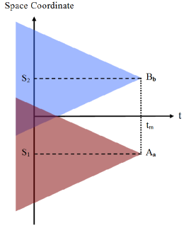
Figure 2: Light cone figure

The elements of reality and the corresponding random variables of the mathematical model are permitted to be functions of the space-time coordinates of the respective light-cones. As parameter random variables we admit not only source parameters but also equipment parameters for each measurement station. What we introduce below is a dependence of the equipment parameters of a given station on the setting vector in the light-cone of that station and an additional dependence on the time of measurement of a clock in the inertial frame of the equipment.

All we need to achieve is to derive a model for Ma-EPR within the space-time of relativity that is not refuted by Bell-type inequalities and agrees with (i) and (ii) in spirit (if not the letter). For this it is only necessary to find an Einstein local model with random variables $A,B,C$ that can not be defined on one common probability space. To show that this is possible we revert to the standard notation using the settings as subscripts and denoting the functions in the two experimental wings by $A_{\bf a},A_{\bf b}$ on one side and $B_{\bf b},B_{\bf c}$ on the other. We continue to permit all functions to be functions of a source parameter $\Lambda$ which may have a time dependence e.g. $\Lambda$ may depend on the time of emission of the correlated pair. However, we also add equipment random variables. Of course, equipment parameters have been discussed before in many research articles. But none of them considered the role of time dependencies of these equipment parameters except our work (see [18]). We permit that the probability densities of these additional random variables depend on the time of measurement $t_{m}$ as shown by a local clock and also to depend on the local setting. We indicate this latter fact by denoting the additional random variable e.g. for setting $\bf a$ by $\Lambda_{\bf a}(t_{m})$ we then have $A_{\bf a}=A_{\bf a}(\Lambda,\Lambda_{\bf a}(t_{m}))$ and similar for the other settings and the $B$’s on the other side e.g. $B_{\bf b}=B_{\bf b}(\Lambda,\Lambda_{\bf b}(t_{m}))$. Notice that all light-cones for different measurement times may contain different $\Lambda_{\bf a}(t_{m})$ even though the setting is the same. No matter how a probabilistic model is conceived, different light-cones can certainly support different probability distributions for the elements of reality. Assume now that as in the Aspect-type experiment the settings on each side are sequentially changed. Because according to relativity this change of settings to take place requires a time interval of length bounded away from 0 by a positive constant $c_{0}$, all light-cone pairs of a sequence of measurements are different and each such experiment may be on a different probability space with a different density of the involved random variables. Furthermore, let $\eta$ be an element of a probability space that determines the random times of measurement i.e. $t_{m}(\eta)$ is the actual measurement time of a given experiment. We now show that physical reasons, derived from the framework of relativity only, necessitate the involvement of different probability spaces if one postulates the existence of time and setting dependent Einstein local equipment parameters.

Theorem2: Assume that there exist a source parameter $\Lambda$ and equipment parameters $\Lambda_{\bf a},\Lambda_{\bf b}$ and $\Lambda_{\bf c}$ such that $\Lambda_{\bf a},\Lambda_{\bf b}$ and $\Lambda_{\bf c}$ not only depend on the setting vectors ${\bf a},\bf b$ and $\bf c$, respectively, but also on the time $t_{m}$ of a given measurement. Here we consider $t_{m}$ to be a random variable $t_{m}=t_{m}(\eta)$. Thus

$$\Lambda_{\bf a}=\Lambda_{\bf a}(t_{m}(\eta))\text{ , }\Lambda_{\bf b}=\Lambda_{\bf b}(t_{m}(\eta))\text{ , }\Lambda_{\bf c}=\Lambda_{\bf c}(t_{m}(\eta))$$ (18)

The source parameter $\Lambda=\Lambda(\omega)$ is permitted to depend on emission time. We assume further that the random variables corresponding to the measurements of spin $A_{\bf a},A_{\bf b},B_{\bf b}$ and $B_{\bf c}$ all equal to $\pm 1$ are functions of the source parameter and of the equipment parameters $\Lambda_{\bf a},\Lambda_{\bf b}$ and $\Lambda_{\bf c}$. Then, under the assumption that the velocity of light in vacuo is an upper limit for the velocities by which the settings can be changed, there is no probability space on which all of

$$A_{\bf a}=A_{\bf a}(\Lambda(\omega),\Lambda_{\bf a}(t_{m}(\eta))$$

$$A_{\bf b}=A_{\bf b}(\Lambda(\omega),\Lambda_{\bf b}(t_{m}(\eta))$$

$$B_{\bf b}=B_{\bf b}(\Lambda(\omega),\Lambda_{\bf b}(t_{m}(\eta))$$

$$B_{\bf c}=B_{\bf c}(\Lambda(\omega),\Lambda_{\bf c}(t_{m}(\eta))$$ (19)

can be consistently defined.

Proof: Let $I$ be any time interval of length $|I|\leq\frac{1}{2}c_{0}$. Let $M$ be a measurable set in the range of $\Lambda$ and let $F,G$ and $H$ be sets in the ranges of $\Lambda_{\bf a}$, $\Lambda_{\bf b}$ and $\Lambda_{\bf c}$ respectively. Then

$$[(\omega,\eta):t_{m}(\eta)\in I,\Lambda(\omega)\in M,\Lambda_{\bf a}(t_{m}(\eta))\in F,\Lambda_{\bf b}(t_{m}(\eta))\in G,\Lambda_{\bf c}(t_{m}(\eta))\in H]$$ (20)

is the impossible event and therefore has probability 0. Recall that $\omega$ signifies the sending out of a particular particle pair from the source. This result simply reflects the impossibility in the space-time of relativity to accomplish two different settings on both sides within the same short time interval and all for the same $\omega$. Hence for each time interval $I$ each of the sixteen probabilities

$$P[(\omega,\eta):t_{m}(\eta)\in I,A_{\bf a}(\cdot)=\pm 1,A_{\bf b}(\cdot)=\pm 1,B_{\bf b}(\cdot)=\pm 1,B_{\bf c}(\cdot)=\pm 1]=0$$ (21)

must vanish. Here $(\cdot)$ denotes the dependence on source and equipment parameters that in turn depend on $\omega$ and $\eta$ respectively just as in Eq.(19). Now let $J$ be a finite but arbitrarily long time interval. Then $J$ can be split up into a large but finite number $N$ of intervals $I_{i},i=1,2,...,N$ with length $|I_{i}|\leq\frac{1}{2}c_{0}$. Then the probability in Eq.(21) with $I$ replaced by $J$ also must vanish because of finite additivity and thus $A_{\bf a},A_{\bf b},B_{\bf b}$ and $B_{\bf c}$ cannot be defined on a common probability space as claimed.

In other words, not only must we have different probability spaces involved in the Aspect-type experiment for mathematical reasons, we must have different probability spaces for physical reasons, the requirements of relativity. We emphasize that none of the assumptions in the above proof imply any synchronization of the measurement times with certain settings. Both settings and measurement times can be chosen randomly, only the measurement times in $S_{1}$ and $S_{2}$ are correlated for any given photon pair.

Note that the essence of Bohr’s discussion is not violated by the above. We just need to view both spin and measurement equipment in the sense of information theory: the measurement outcome is really not the single consequence of the source information $\lambda$ that characterizes particle properties but also that of the measurement equipment and the corresponding $\lambda_{\bf a}(t_{m})$ etc.. These equipment parameters correspond to the use of decoding machines in information theory [20]. Both the source information content together with that of the decoding machines or equipment parameters (that involve different probability spaces) determine the measurement outcomes i.e. the values $\pm 1$ that the functions $A_{\bf a}$ etc. assume. In a larger sense this fulfills the spirit of Bohr. The spin does not really exist before the measurement, but only in the very moment of measurement is the outcome determined (decoded) and can not be separated from the equipment and act of measurement. The contextuality is implicitly contained in the dependence of the probability densities of the various variables on measurement time. For example, it is now incorrect to say that it makes no difference if one measures with setting $\bf b$ or setting $\bf c$ on the other side. It does make a difference because one necessarily makes these different measurements during different time intervals. The measurements in both wings are also performed at the same clock-time or at least at correlated clock-times which opens the possibility of correlations between the two wings even though the settings are randomly chosen.

What is the meaning then of the Aspect et al. [8] experiment in view of the above discussions? If one assumes that this experiment is free from any problems related to non-ideal experimental conditions and if one assumes that a space-time explanation must be possible then the Aspect et al. experiment has proven the existence of setting and time dependent equipment parameters.

7 Conclusion

We have shown that the inequalities of Bell can be derived as special cases of a more general theorem found by Bass ten years earlier. We have further shown that the Bell inequalities are valid if and only if the three random variables involved can actually be defined on a common probability space. As a consequence the Bell theorem is correct at least for the following systems of hidden variables, in the sense that these systems can be ruled out:

1. Source parameter $\Lambda$ only,

2. Source parameter $\Lambda$ and equipment parameters $\Lambda_{\bf a}$, $\Lambda_{\bf b}$ and $\Lambda_{\bf c}$ that depend only on the respective settings.

On the other hand, equipment parameters that depend on the measurement times as well as on the respective instrument settings can not be ruled out. A space-time explanation of the Aspect et al. experiment is therefore not ruled out by Bell’s inequalities. Any such space-time explanation can not rely on source parameters only but must involve a certain type of time and setting dependent equipment parameter random variables. Thus, the validity of the Bell inequalities for objective local parameter spaces has not been proven by any of the proofs reported in the literature [3], [5], [17].

8 Acknowledgement

The authors would like to thank M. Aschwanden for creating the figures of the manuscript and helpful suggestions. Support of the Office of Naval Research (N00014-98-1-0604) is gratefully acknowledged.

References

- [1] A. Einstein, B. Podolsky, and N. Rosen, Phys. Rev. Vol. 47, 777 (1935).
- [2] N. Bohr, Phys. Rev. Vol. 48, 696 (1935).
- [3] J.S. Bell, ”Speakable and Unspeakable in Quantum Mechanics”, pp 1-13, Cambridge University Press (1993)
- [4] J. S. Bell, Physics, Vol. 1, 195 (1964).
- [5] A. J. Leggett, The Problems of Physics, Oxford University Press, pp 144-172 (1987).
- [6] D. Bohm and Y. Aharonov, Phys. Rev. 108, 1070, (1957)
- [7] D. Bohm and B. J. Hiley, Nonlocality in Quantum Theory Understood in Terms of Einstein’s Nonlinear Field Approach, Foundations of Physics 11 (1981) 529 - 546.
- [8] A. Aspect, J. Dalibard and G. Roger, Phys. Rev. Letters 49, 1804-1807 (1982).
- [9] W. Moore, Schrödinger, Cambridge University Press, paperback edition p 312 (1993).
- [10] J. Bass, C. R. Acad. Sci.(Paris), 839-841 (1955).
- [11] N.N. Vorob’ev,Dokl Akad. Nauk SSR 124, 253-256 (1959)
- [12] N. N. Vorob’ev, Theory of Probability and its Applications VII, 147-162 (1962).
- [13] E. D. Schell, Proc. 2-nd Symp. Lin. Programming, Washington, Vol. 2, 615-642 (1955).
- [14] W. Feller, “An Introduction to Probability Theory and its Applications” Vol 1, 3rd edition, Wiley Series in Probability and Mathematical Statistics, pp1-9 (1968)
- [15] A. Fine, J. Math. Phys. 23, 1306-1310 (1982).
- [16] N. J. Cerf and C. Adami, Phys. Rev. A 55, 3371-3374 (1997)
- [17] A. Peres, “Quantum Theory: Concepts and Methods”, Kluewer Academic Publishers (1995)
- [18] K. Hess and W. Philipp, Proceedings of the National Academy of Sciences (USA) 101 1799-1805 (2004).
- [19] J. F. Clauser, R. A. Holt, M. A. Horne and A. Shimony, Phys. Rev. Letters Vol. 23, 880 (1969).
- [20] C. E. Shannon and W. Weaver, The Mathematical Theory of Communication, University of Illinois Press, Urbana and Chicago, pp 81-86 (1998)