Abstract

New type of tomographic probability distribution which contains complete information on the density matrix (wave function) related to the Fresnel transform of the complex wave function is introduced. Relation to symplectic tomographic probability distribution is elucidated. Multimode generalization of the Fresnel tomography is presented. Examples of applications of the present approach are given.

keywords: tomographic map, phase space, Wigner function, Bose–Einstein condensate, Fresnel tomogram.

1 Introduction

Recently symplectic tomography introduced in quantum optics [1] and signal analysis [2, 3] was extended to the problem of soliton solutions for some nonlinear dynamical equations like nonlinear Schrödinger equation [4, 5] including the study of solitons in Bose–Einstein condensate [6] described by Gross–Pitaevsky equation [7]. The name “symplectic tomography” is related to using in the approach standard symplectic group transformations in phase space (linear canonical transformation in position and momentum preserving Poisson brackets in classical case and commutator in quantum case). The symplectic tomographic map associates with a function (analytic signal, soliton solution, etc.) a specific probability distribution function (symplectic tomogram) containing the same information on the signal as the initial function. It was found in [4, 5, 6] that due to the structure of symplectic tomogram depending on three real coordinates, one can construct another probability distribution (Fresnel tomogram). This tomogram depends on two real variables but information contained in the Fresnel tomogram is sufficient to reconstruct the initial function for which this tomogram is known. The inverse formula which permits to make explicit reconstruction of the initial function (signal, soliton, etc.) was not written until now and it is one of the aims of this work, namely, to present the reconstruction formula. Another goal of the work is to extend the Fresnel tomography to two-particle (multiparticle) systems to be able to consider in the tomographic representation, e.g., soliton solutions of nonlinear equations for 2D and 3D cases.

The paper is organized as follows.

In Section 2, we review the symplectic tomography scheme both for 1D case and multidimensional case. In Section 3, we present the basic concept of the Fresnel tomography for 1D case while in Section 4 we present an extension of the Fresnel tomographic approach to multidimensional problems. In Section 5, we apply our method to the case of 1D chirped Gaussian wave functions. Finally, the conclusions are summarized in Section 6.

2 Symplectic tomograms

Below we present symplectic tomograms associated with a complex function $\psi(x)$ describing either a quantum normalized state or analytic signal or soliton solution of a nonlinear equation. The tomogram is given by the formula [2]

$$w(X,\mu,\nu)=\frac{1}{2\pi|\nu|}\left|\int\psi(y)\exp\left(\frac{i\mu}{2\nu}\,y^{2}-\frac{iX}{\nu}\,y\right)\,dy\right|^{2}.$$ (1)

One can see that the tomogram which depends on three real variables has the homogeneity property

$$w(\lambda X,\lambda\mu,\lambda\nu)=\frac{1}{|\lambda|}\,w(X,\mu,\nu).$$ (2)

The inverse transform which relates the tomogram to the complex function (density matrix) reads [8]

$$\psi(X)\psi^{*}(X^{\prime})=\frac{1}{2\pi}\int w(Y,\mu,X-X^{\prime})\exp\left[i\left(Y-\mu\,\frac{X+X^{\prime}}{2}\right)\right]\,d\mu\,dY.$$ (3)

Since one can reconstruct the density matrix in view of the known symplectic tomogram, all other characteristics like Wigner–Ville function [9, 10] can be also expressed in terms of the symplectic tomogram [11, 12]

$$W_{\psi}(q,p)=\int w(X,\mu,\nu)\exp\Big{[}i(X-\mu q-\nu p)\Big{]}\,\frac{dX\,d\mu\,d\nu}{(2\pi)^{2}}\,,$$ (4)

where

$$W_{\psi}(q,p)=\frac{1}{2\pi}\int\psi\left(q+\frac{u}{2}\right)\psi^{*}\left(q-\frac{u}{2}\right)e^{-ipu}du.$$

The Wigner function is normalized $W_{\psi}(q,p)\,dq\,dp=1$. The symplectic tomogram provides the possibility to find the optical tomogram simply taking the parameter of the tomogram in the form $\mu=\cos\theta$, $\nu=\sin\theta$. One arrives at the formula for the optical tomogram in the form

$$w(X,\theta)=\frac{1}{2\pi|\sin\theta|}\left|\int\psi(y)\exp\left(\frac{i\,\cot\theta}{2}\,y^{2}-\frac{iX}{\sin\theta}\,y\right)dy\right|^{2}.$$ (5)

Thus optical tomogram can be used in order to reconstruct Wigner function [13, 14] by means of Radon transform [15].

The generalization of symplectic tomogram to the multidimensional case is straightforward.

To provide this generalization we introduce the following notation.

There are three real vectors

$$\vec{X}=(X_{1},X_{2},\ldots,X_{N}),\quad\vec{\mu}=(\mu_{1},\mu_{2},\ldots,\mu_{N}),\quad\vec{\nu}=(\nu_{1},\nu_{2},\ldots,\nu_{N})$$

and all the components of these vectors vary from $-\infty$ to $\infty$. The tomogram $w(\vec{X},\vec{\mu},\vec{\nu})$ associated to a complex function $\psi(\vec{x})$, $\vec{x}=(x_{1},x_{2},\ldots,x_{N})$ reads

$$w(\vec{X},\vec{\mu},\vec{\nu})=\left(\prod_{k=1}^{N}\frac{1}{2\pi|\nu_{k}|}\right)\left|\int\psi(\vec{y})\prod_{j=1}^{N}\exp\left(\frac{i\mu_{j}}{2\nu_{j}}\,y_{j}^{2}-\frac{iX_{j}}{\nu_{j}}\,y_{j}\right)\,d\vec{y}\right|^{2}.$$ (6)

The inverse formula has the form

$$\psi(\vec{X})\psi^{*}(\vec{X}^{\prime})=\left(\frac{1}{2\pi}\right)^{N}\int w(\vec{Y},\vec{\mu},\vec{X}-\vec{X}^{\prime})\left\{\prod_{k=1}^{N}\exp\left[i\left(Y_{k}-\mu_{k}\,\frac{X_{k}+X_{k}^{\prime}}{2}\right)\right]\right\}\,d\vec{\mu}\,d\vec{Y}.$$ (7)

3 Fresnel tomography in 1D case

In [4, 16, 17] the Fresnel tomogram $w_{F}(X,\nu)$ was introduced

$$w_{F}(X,\nu)=\left|\frac{1}{\sqrt{2\pi i\nu}}\int\exp\frac{i(X-y)^{2}}{2\nu}\psi(y)\,dy\right|^{2}.$$ (8)

Another version of Fresnel tomography based on using the Fresnel integral to reconstruct Wigner function of quantum state was suggested in [18].

Since the symplectic tomogram $w(X,\mu,\nu)$ is homogeneous function, there exists the relation

$$w(X,\mu,\nu)=\frac{1}{|\mu|}\,w_{F}\left(\frac{X}{\mu}\,,\frac{\nu}{\mu}\right).$$ (9)

This means that if one knows Fresnel tomogram $w_{F}(X^{\prime},\nu^{\prime})$, the symplectic tomogram is obtained by the substitution of the arguments of this function

$$X^{\prime}\to\frac{X}{\mu}\,,\qquad\nu^{\prime}\to\frac{\nu}{\mu}$$

and multiplication of the obtained function by the factor $|\mu|^{-1}$. The formulated relations provide the inverse formula to reconstruct density matrix by expressing it in terms of Fresnel tomogram

$$\psi(\vec{X})\psi^{*}(\vec{X}^{\prime})=\frac{1}{2\pi}\int\frac{1}{|\mu|}\,w_{F}\left(\frac{Y}{\mu}\,,\frac{X-X^{\prime}}{\mu}\right)\exp\left[i\left(Y-\mu\,\frac{X+X^{\prime}}{2}\right)\right]\,d\mu\,dY.$$ (10)

One can also reconstruct the Wigner function expressing it in terms of Fresnel tomogram

$$W(q,p)=\frac{1}{(2\pi)^{2}}\int\frac{1}{|\mu|}\,w_{F}\left(\frac{X}{\mu}\,,\frac{\nu}{\mu}\right)\exp\,[-i(\mu q+\nu p-X)]\,d\mu\,d\nu\,dX.$$ (11)

The inverse formula obtained gives a possibility to find the Wigner function and the density matrix in the position representation if one knows the Fresnel tomographic probability distribution $w_{F}(X,\nu)\geq 0$, which satisfies the normalization condition

$$\int w_{F}(X,\nu)\,dX=1.$$ (12)

4 Fresnel tomogram for multipartite system

Let us introduce the Fresnel tomogram for function $\psi(\vec{x})$ depending on several variables. This tomogram can be defined in terms of symplectic tomogram, i.e.,

$$w_{F}(\vec{X},\vec{\nu})=w(\vec{X},\vec{\mu}=1,\vec{\nu}),$$ (13)

where we have symplectic tomogram and $\vec{\mu}=\vec{1}$ means that the vector $\vec{\mu}$ is taken to have all the components equal to one. Thus the Fresnel tomogram is expressed in terms of the complex function $\psi(\vec{x})$ as follows:

$$w_{F}(\vec{X},\vec{\nu})=\left|\prod_{k=1}^{N}\frac{1}{\sqrt{2\pi i\nu_{k}}}\int\psi(\vec{y})\left(\prod_{j=1}^{N}\exp\frac{i(X_{j}-y_{j})^{2}}{2\nu_{j}}\right)d\vec{y}\right|^{2}.$$ (14)

To get the inverse of the above transform, we have to use the multidimensional analog of relation (9) which reads

$$w(\vec{X},\vec{\mu},\vec{\nu})=\frac{1}{|\mu_{1}\mu_{2}\cdots\mu_{N}|}\,w_{F}\left(\vec{X}_{\vec{\mu}}\,,\vec{\nu}_{\vec{\mu}}\right),$$ (15)

where vectors in the argument of Fresnel tomogram have the components

$$\vec{X}_{\vec{\mu}}=\left(\frac{X_{1}}{\mu_{1}}\,,\frac{X_{2}}{\mu_{2}}\,,\ldots,\frac{X_{N}}{\mu_{N}}\right),\qquad\vec{\nu}_{\vec{\mu}}=\left(\frac{\nu_{1}}{\mu_{1}}\,,\frac{\nu_{2}}{\mu_{2}}\,,\ldots,\frac{\nu_{N}}{\mu_{N}}\right).$$

Using relation (15) one can construct the expression of the density matrix in terms of the Fresnel tomogram analogous to 1D expression (10)

$$\psi(\vec{X})\psi^{*}(\vec{X}^{\prime})=\int\frac{d\vec{\mu}\,d\vec{Y}}{(2\pi)^{N}}\,w_{F}\left(\vec{Y}_{\vec{\mu}},\vec{X}_{\vec{\mu}}-\vec{X^{\prime}}_{\vec{\mu}}\right)\prod_{j=1}^{N}\frac{1}{|\mu_{j}|}\,\exp\left(iY_{j}-\mu_{j}\,\frac{X_{j}+X^{\prime}_{j}}{2}\right).$$ (16)

5 The chirped Gaussian case

In order to verify the validity of the method, we have numerically simulated the reconstruction of a 1D complex Gaussian chirped field (GCF) given by the following normalized form:

$$\psi(x)=\left({2\over\pi\sigma^{2}}\right)^{1/4}\exp\left[-{x^{2}\over\sigma^{2}}+i\alpha x^{2}\right]$$ (17)

having a chirp $\alpha$ and a width determined by the parameter $\sigma$. The above state is also known as correlated coherent state [19]. According to Eq. (3) the complex field given by Eq. (17) can be retrieved from its tomographic representation $w(X,\mu,x)$ by the following inversion integral:

$$\psi(x)\psi^{*}(0)={1\over 2\pi}\int\int w(X,\mu,x)\exp\left[i\left(X-\mu x/2\right)\right]\,dX\,d\mu.$$ (18)

The GCF tomogram can be calculated from Eqs. (1) and (17). The Gaussian distribution can be integrated and the tomogram can be written in the following form using, according to the notation of the previous sections, the symbol $\nu$ instead of $x$

$$w(X,\mu,\nu)=\sqrt{2\sigma^{2}\over\pi\left[4\nu^{2}+\sigma^{2}\left(\mu+2\alpha\nu\right)^{2}\right]}\,\exp\left\{-{2\sigma^{2}X^{2}\over 4\nu^{2}+\sigma^{4}\left(\mu+2\alpha\nu\right)^{2}}\right\}.$$ (19)

Equation (19) shows that the GCF tomogram is still characterized by a Gaussian distribution law but its width $\omega$ is, in general, different from the width of the original GCF and it can be expressed in terms of the phase-space variables $\mu$ and $\nu$, chirp parameter $\alpha$, and width $\sigma$, namely,

$$\omega^{2}={\left(\mu+2\alpha\nu\right)^{2}\sigma^{2}+4\nu^{2}\over 2\sigma^{2}}\,.$$ (20)

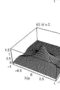
Figure 1: 3D plot of the tomogram distribution $w(X/\mu,1,\nu/\mu)$ of the Gaussian chirped wave function for a width of the Gaussian $\sigma=1$ and for increasing values of the chirp parameter $\alpha=0.5$ (a), 1 (b), 2 (c) and 3 (d).

It can be easily verified that the tomogram $w(X,\mu,\nu)$ in Eq. (19) coincides with the tomogram of a Gaussian field without chirp ($\alpha=0$) computed for the values of the phase-space variables $\mu^{{}^{\prime}}=\mu+2\alpha\nu$ and $\nu^{{}^{\prime}}=\nu$. We can admit a different transformation of the phase space, taking into account that the tomographic representation of the GCF can be also obtained from that of a Gaussian field without chirp with $\mu^{{}^{\prime}}=\mu$ and $\nu^{{}^{\prime}}=\nu\mu/(\mu+2\alpha\nu)$. In both instances, the effect of the chirp is that of shifting one of the two values of the phase-space variables while leaving unaltered the other one. To illustrate the behaviour of the GCF tomogram, we have displayed in Fig. 1 the 3D distribution of the tomographic map $w(X/\mu,1,\nu/\mu)$ for increasing values of the chirp parameter. This representation of the tomogram in terms of two parameters $X/\mu$ and $\nu/\mu$ rather than three is quite convenient since it allows one a clear visualization of the tomographic map in the 2D phase-space plane ($X/\mu$, $\nu/\mu$). Indeed, recalling the general homogeneity property of the tomogram we can obtain complete dependence of the tomogram from its three space variables by virtue of Eq. (9):

$$w(X,\mu,\nu)={1\over|\mu|}\,w(X/\mu,1,\nu/\mu).$$ (21)

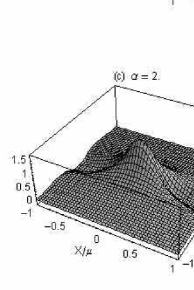
Figure 2: 3D plot of the tomogram distribution $w(X/\mu,1,\nu/\mu)$ of the Gaussian chirped wave function for a width of the Gaussian $\sigma=0.5$ and for increasing values of the chirp parameter $\alpha=0.5$ (a), 1 (b), 2 (c) and 3 (d).

According to the Fresnel-based interpretation of the optical tomogram discussed in the previous section, $w(X/\mu,1,\nu/\mu)$ represents the GCF intensity at distance $\nu$ and Eq. (21) tells us that the general dependence of the tomogram of its three real variables $X$, $\mu$, and $\nu$ can be recovered from a set of measurements of the intensity distributions of the propagated GCF performed at different distances with a varying scale factor $1/|\mu|$. Equation (21) can be verified immediately from the defining expression of the GCF tomogram given by Eq. (19). Figure 1 shows clearly that tomographic distributions shrink in the phase space with increasing the chirp parameter of the Gaussian field. The numerical results have been obtained for a GCF of width $\sigma=1$. In Fig. 2 we display the plots of the tomograms for the same set of values of Fig. 1 except that now the width of the GCF is $\sigma=0.5$. As can be seen by comparing Figs. 1 and 2, the shrinking of the 3D tomographic distribution in the phase space with increasing the chirp parameter is less pronounced when reducing the GCF width. A computationally efficient method for retrieving the wave function makes direct use of the inversion integral given by Eq. (18) which allows one to determine $\psi(x)$ up to the complex constant quantity $\psi(0)^{*}$. The method employs the fast Fourier transform (FFT) algorithm for computing the two-dimensional Fourier transform $\hat{w}(\omega_{X},\omega_{\mu},\nu)$ of the tomogram, namely,

$$\hat{w}(\omega_{X},\omega_{\mu},\nu)={1\over 2\pi}\int_{-\infty}^{\infty}\int_{-\infty}^{\infty}w(X,\mu,\nu)\exp\left[i\left(\omega_{X}X+\omega_{\mu}\mu\right)\right]\,dXd\mu,$$ (22)

where $\omega_{X}$ and $\omega_{\mu}$ are the spatial frequencies corresponding to the phase-space variables $X$ and $\mu$ of the tomogram. The inversion integral is a particular case of the two-dimensional Fourier transform of the tomogram given by Eq. (22). In fact, we have

$$\psi(\nu)\psi(0)^{*}=\hat{w}(1,-\nu/2,\nu).$$ (23)

Equation (23) shows that we can determine the complex quantity $\psi(\nu)\psi(0)^{*}$ from the values of two-dimensional Fourier transform of the tomogram at frequencies $\omega_{X}$ and $\omega_{\mu}$, where $\nu$ is allowed to vary in the range along which the tomographic measurements are performed. In principle, this procedure works well for reconstructing a wave field, if we have a sufficient number of sampled values of the tomographic distribution $w(X,\mu,\nu)$, i.e., if the sampling rate is at least larger than twice the Nyquist rate. In this case, the discrete two-dimensional Fourier transform $\hat{w}(r\Delta\omega_{X},s\Delta\omega_{\mu})$ corresponding to the continuous Fourier integral given by Eq. (22) can be written in the following form:

$$\hat{w}(r\Delta\omega_{X},s\Delta\omega_{\mu})=\Delta X\Delta\mu~{}\sum_{n=0}^{N-1}\sum_{m=0}^{N-1}~{}w(n\Delta X,m\Delta\mu,\nu)\exp\left[-2\pi i\left({rn\over N}+{sm\over M}\right)\right],$$ (24)

where $r,s$ and $n,m$ are integer numbers, $\Delta X$ and $\Delta\mu$ are the sampling intervals in the ($X,\mu$) phase space and $\Delta\omega_{X}$ and $\Delta\omega_{\mu}$ are the corresponding sampling intervals in the frequency space. Equation (24) allows one to compute a matrix of $N^{2}$ complex numbers $\hat{w}(r\Delta\omega_{X},s\Delta\omega_{\mu})$ from the sampled values $w(n\Delta X,m\Delta\mu,\nu)$ of the tomogram of the wave function via the discrete two-dimensional fast Fourier transform (FFT) algorithm. It should be remarked that in order to obtain accurate reconstruction of the wave function $\psi(\nu)$, the two-dimensional FFT algorithm needs to be repeatedly applied to every two-dimensional tomographic distribution corresponding to each $\nu$ value in the considered range and, if high accuracy is required, even this FFT-based reconstruction method becomes computationally expensive. However, in many cases of interest, symmetry consideration allows one to simplify somewhat the task through the consideration of a reduced set of sampled values of the tomogram. In the GCF case, the two-dimensional Fourier transform $\hat{w}(\omega_{X},\omega_{\mu},\nu)$ can be readily obtained in the following form:

$$\hat{w}(\omega_{X},\omega_{\mu},\nu)=\sqrt{2\over\pi\sigma^{2}\omega_{X}^{2}}\exp\left[-{\nu^{2}\over 2}\left({\omega_{X}\over\sigma}\right)^{2}-{2\over\sigma^{2}}\left({\omega_{\mu}\over\omega_{X}}\right)^{2}-2i\alpha\omega_{\mu}\nu\right].$$ (25)

By using Eq. (25) it can be easily verified that Eq. (23) gives correctly $\psi(\nu)\psi(0)^{*}$ with the wave function $\psi(\nu)$ given by the Gaussian chirped field in Eq. (17).

6 Conclusions

We summarize the main results of the paper.

We obtained the inverse formula which in explicit form reconstructs the wave function, density matrix and Wigner function from the known Fresnel tomographic probability distribution function. The Fresnel tomogram can be used to measure the phase of radiation by measuring the intensity of the radiation.

We introduced Fresnel tomogram for multimode system and found reconstruction formula for wave function and density matrix in terms of the tomograms for this case too. An example of soliton solution used also in analyzing some states of Bose–Einstein condensate can be studied from the viewpoint of Fresnel tomography [5, 6].

The symplectic tomography [1] has as a partial case the optical tomography procedure. In this work, we clarified that there exists another important partial case of the symplectic tomography which is named Fresnel tomography. This mean that there exists a connection of Fresnel tomography with well-developed optical tomography scheme. The tomographic probability of optical tomography scheme is connected with Fresnel tomogram by the relation:

$$w(x,\cos\theta,\sin\theta)=\frac{1}{|\cos\theta|}\,w_{F}\left(\frac{X}{\sin\theta}\,,\cot\theta\right).$$

One can generalize this formula to multidimensional case.

References

- [1] S. Mancini, V. I. Man’ko and P. Tombesi 1995 Quantum Semiclass. Opt. 7 615; Phys. Lett. A, 213, 1 (1996); Found. Phys., 27, 801 (1997).
- [2] V. I. Man’ko and R. V. Mendes 1999 Phys. Lett. A 263 53
- [3] M. A. Man’ko 1999 J. Russ. Laser Res. 20 226; 2000 ibid 21 411; 2001 ibid 22 505; 168; 2002 ibid 23 433
- [4] S. De Nicola, R. Fedele, M. A. Man’ko and V. I. Man’ko 2003 J. Opt. B: Quantum Semiclass. Opt. 5 95
- [5] S. De Nicola, R. Fedele, M. A. Man’ko and V. I. Man’ko 2003 ”Wigner picture and tomographic representation of envelope solitons” in: M. J. Ablowitz, M. Boiti and F. Pempinelli (eds.) “Proceedings of the International Workshop ‘Nonlinear Physics: Theory and Experiment. II’ (Gallipoli, Lecce, Italy, 27 June – 6 July 2002)” (Singapore: World Scientific), p. 372
- [6] S. De Nicola, R. Fedele, M. A. Man’ko and V. I. Man’ko 2004 J. Russ. Laser Res. 25 1; 2003 European J. Phys. B 36 385
-
[7]
E. P. Gross 1961 Nuovo Cim. 20 454
L. P. Pitaevskii 1961 Sov. Phys. JETP 1961 13 451 - [8] V. I. Man’ko, L. Rosa and P. Vitale 1998 Phys. Rev. A 57 3291
- [9] E. P. Wigner 1932 Phys. Rev. 40 749
- [10] J. Ville 1948 Cables et Transmission 2 61
- [11] G. M. D’Aiano, S. Mancini, V. I. Man’ko and P. Tombesi 1996 Quantum Semiclass. Opt. 8 1017
- [12] R. Fedele and V. I. Man’ko 1999 Phys. Rev. E 60 6042
- [13] J. Bertrand and P. Bertrand 1987 Found. Phys. 17 397
- [14] K. Vogel and H. Risken 1989 Phys. Rev. A 40 2847
- [15] J. Radon 1917 Ber. Verh. Sachs. Akad. 69 262
- [16] M. A. Man’ko 2002 “Wigner function and tomograms in signal processing and quantum computing” Talk at the Wigner Centennial Conference (Pecs, Hungary, July 2002)
- [17] S. De Nicola, R. Fedele, M. A. Man’ko and V. I. Man’ko 2002 “Tomographic analysis of envelope solitons: Concepts and applications” in “Abstracts of the International Workshop ‘Optics in Computing’. International Optical Congress ‘Optics XXI Centuary’ (St. Petersburg, Russia, 14–18 November 2002)”
- [18] P. Lougovski, E. Solano, Z. M. Zhang, H. Walter, H. Mack and W. P. Schleich 2002 “Fresnel transform: an operational definition of the Wigner function” Eprint quant-ph/0206083; 2003 Phys. Rev. Lett. 91 010401-1; O. Crasser, H. Mack and W. P. Schleich 2004 “Is Fresnel optics quantum mechanics in phase space?” Eprint quant-ph/0402115
- [19] V. V. Dodonov, E. V. Kurmyshev and V. I. Man’ko 1980 Phys. Lett. A 79 150