Static and Dynamic Casimir Effect Instabilities

Abstract

The static Casimir effect concerns quantum electrodynamic induced Lamb shifts in the mode frequencies and thermal free energies of condensed matter systems. Sometimes, the condensed matter constitutes the boundaries of a vacuum region. The static frequency shift effects have been calculated in the one photon loop perturbation theory approximation. The dynamic Casimir effect concerns two photon radiation processes arising from time dependent frequency modulations again computed in the one photon loop approximation. Under certain conditions the one photon loop computation may become unstable and higher order terms must be invoked to achieve stable solutions. This stability calculation is discussed for a simple example dynamical Casimir effect system.

1 Introduction

The Casimir effect concerns the Lamb shifts in the frequency of radiation modes due to the interaction between photon modes and electrical currents. The photon mode Lagrangian is discussed in Sec.2. Mode frequency shifts induce changes in the free energy which in the zero temperature limit[1, 2] reduce to changes in the zero point energy[3, 4] $\delta E_{0}=(\hbar/2)\sum_{a}\delta\Omega_{a}$. The Lamb frequency shifts are usually small and can be understood from a perturbation theory viewpoint. Such damping is discussed in Sec.3. The conventional Casimir effect theory thereby considers Feynman diagram corrections to the free energy containing one photon loop[5, 6]. In Sec.4 it is shown how a one loop instability can arise if the coupling between a photon oscillation mode and the surrounding currents is too strong.

If the damping functions and frequency shifts are also oscillating functions of time, then (over and above single photon absorption and emission processes) there is the absorption and emission of photon pairs[8]. The photon pair processes constitute a dynamical Casimir effect[7, 9]. Frequency modulations tend to heat up the cavity. In Sec.5, the noise temperature description is discussed. In Sec.6, the heating of a cavity mode by periodic frequency modulation is explored. In an unstable regime, the temperature of (say) a microwave cavity mode grows exponentially. The implied purely theoretical microwave oven would be much more hot than that which could be observed in experimental reality. Nonlinear higher loop photon processes producing dynamic microwave intensity stability are discussed in Sec.7.

2 Lagrangian Circuit Mode Description

Our purpose in this section is to provide a Lagrangian description of a single microwave cavity mode which follows from the action principle formulation of electrodynamics[10]. For this purpose we employ the Coulomb gauge, $div{\bf A}_{mode}=0$, for the vector potential. The vector potential representing the cavity mode may be written

$${\bf A}_{mode}({\bf r},t)=\Phi(t){\bf K}({\bf r}).$$ (1)

The mode electromagnetic fields are then given by

$${\bf E}_{mode}({\bf r},t)=-\frac{1}{c}\left[\frac{{\bf A}_{mode}({\bf r},t)}{\partial t}\right]=-\frac{\dot{\Phi}(t)}{c}{\bf K}({\bf r}),$$

$${\bf B}_{mode}({\bf r},t)=curl{\bf A}_{mode}({\bf r},t)=\Phi(t)\ curl{\bf K}({\bf r}).$$ (2)

The Lagrangian

$$L_{field}=\frac{1}{8\pi}\int_{cavity}\left[\left|{\bf E}_{mode}({\bf r},t)\right|^{2}-\left|{\bf B}_{mode}({\bf r},t)\right|^{2}\right]d^{3}{\bf r}$$ (3)

describes the mode in terms of a simple oscillator circuit. The capacitance $C$ and inductance $\Lambda$ of the circuit are defined, respectively, by

$$C=\frac{1}{4\pi}\int_{cavity}\left|{\bf K}({\bf r})\right|^{2}d^{3}{\bf r},$$

$$\frac{1}{\Lambda}=\frac{1}{4\pi}\int_{cavity}\left|curl{\bf K}({\bf r})\right|^{2}d^{3}{\bf r}.$$ (4)

The circuit electromagnetic field Lagrangian follows from Eqs.(2), (3) and (4). It is of the simple $\Lambda C$ oscillator form

$$L_{field}(\dot{\Phi},\Phi)=\frac{C}{2c^{2}}\dot{\Phi}^{2}-\frac{1}{2\Lambda}\Phi^{2},$$ (5)

wherein the bare circuit frequency obeys

$$\Omega_{\infty}^{2}=\frac{c^{2}}{\Lambda C}\ .$$ (6)

The interactions between cavity wall currents and an electromagnetic mode are conventionally described by

$$L_{int}=\frac{1}{c}\int{\bf J}\cdot{\bf A}_{mode}d^{3}{\bf r},$$

$$L_{int}=\frac{1}{c}I\Phi,$$

$$I(t)=\int{\bf J}({\bf r},t)\cdot{\bf K}({\bf r})d^{3}{\bf r},$$ (7)

where the current $I$ drives the oscillator circuit.

In total, the circuit mode Lagrangian follows from Eqs.(5) and (7) as

$$L=\frac{C}{2c^{2}}\dot{\Phi}^{2}-\frac{1}{2\Lambda}\Phi^{2}+\frac{1}{c}I\Phi+L^{\prime}$$ (8)

wherein $L^{\prime}$ describes all of the other degrees of freedom which couple into the mode coordinate. Maxwell’s equations for a single microwave mode then takes the form

$$\frac{d}{dt}\left(\frac{\partial L}{\partial\dot{\Phi}}\right)=\left(\frac{\partial L}{\partial\Phi}\right),$$

$$C\left(\ddot{\Phi}+\Omega_{\infty}^{2}\Phi\right)=cI.$$ (9)

The damping of the oscillator will first be discussed from a classical electrical engineering viewpoint and only later from a fully quantum electrodynamic viewpoint.

3 Oscillator Circuit Damping

From an electrical engineering viewpoint, let us consider a small external current source $\delta I_{ext}$ which drives the mode coordinate $\delta\Phi$. Eq.(9) now reads

$$\frac{C}{c^{2}}\delta\ddot{\Phi}+\frac{1}{\Lambda}\delta\Phi=\frac{1}{c}\delta I=\frac{1}{c}\left(\delta I_{ext}+\delta I_{ind}\right)$$ (10)

were $\delta I_{ind}$ is the current induced by the coordinate response $\delta\Phi$. In the complex frequency $\zeta$ domain we have in (the upper half ${\Im}m\ \zeta>0$ plane)

$$\delta I_{ext}(t)={\Re}e\left\{\delta I_{ext,\zeta}e^{-i\zeta t}\right\}$$

$$\delta\Phi(t)={\Re}e\left\{\delta I_{ext,\zeta}{\cal D}(\zeta)e^{-i\zeta t}\right\}.$$ (11)

The induced current is determined by the “surface admittance” $Y(\zeta)$ of the cavity walls; In detail

$$\delta I_{ind}(t)=-\frac{1}{c}\int_{0}^{\infty}{\cal G}(t^{\prime})\delta\dot{\Phi}(t-t^{\prime})dt^{\prime},$$

$$Y(\zeta)=\int_{0}^{\infty}e^{i\zeta t}{\cal G}(t)dt,$$ (12)

so that

$$\left\{-\frac{C}{c^{2}}\zeta^{2}+\frac{1}{\Lambda}-\frac{i\zeta}{c^{2}}Y(\zeta)\right\}{\cal D}(\zeta)=\frac{1}{c}\ ,$$

$$-i\zeta\varepsilon(\zeta)C=-i\zeta C+Y(\zeta),$$ (13)

wherein the effective frequency dependent capacitance $\varepsilon(\zeta)C$ determines the mode dielectric response function $\varepsilon(\zeta)$. The retarded propagator for the mode in the frequency domain obeys

$${\cal D}(\zeta)=\frac{\Lambda}{c}\left[\frac{\Omega_{\infty}^{2}}{\Omega_{\infty}^{2}-\zeta^{2}-\Pi(\zeta)}\right]$$ (14)

wherein the “self energy” $\Pi(\zeta)$ is determined by the induced current admittance via

$${\Pi(\zeta)}=\frac{i\zeta Y(\zeta)}{C}\ .$$ (15)

The self energy describes both frequency shift and damping properties of the mode.

Causality dictates that all engineering response functions obey analytic dispersion relations (${\Im}m\ \zeta>0$) of the form

$${\cal D}(\zeta)=\frac{2}{\pi}\int_{0}^{\infty}\frac{\omega{\Im}m{\cal D}(\omega+i0^{+})d\omega}{\omega^{2}-\zeta^{2}}\ ,$$

$$\Pi(\zeta)=\frac{2}{\pi}\int_{0}^{\infty}\frac{\omega{\Im}m\Pi(\omega+i0^{+})d\omega}{\omega^{2}-\zeta^{2}}\ .$$ (16)

The damping rate for the oscillation is determined by

$${\Im}m\Pi(\omega+i0^{+})=\omega{\Re}e\Gamma(\omega+i0^{+})=\frac{\omega{\Re}eY(\omega+i0^{+})}{C}\ .$$ (17)

The shifted frequency,

$$\Omega_{0}^{2}=\Omega_{\infty}^{2}-\Pi(0),$$ (18)

obeys the dispersion relation sum rule The shifted frequency is related to the damping rate via the sum rule

$$\Omega_{\infty}^{2}=\Omega_{0}^{2}+\frac{2}{\pi}\int_{0}^{\infty}{\Re}e\Gamma(\omega+i0^{+})d\omega,$$ (19)

which follows from Eqs.(15) - (18). Finally, the the quality factor $Q$ for the mode frequency $\Omega_{0}$ is well defined as

$$\frac{\Omega_{0}}{Q}={\Re}e\Gamma(\Omega_{0}+i0^{+})$$ (20)

if and only if the mode is under damped by a large margin; e.g. $Q>>1$. On the other hand, if the damping is sufficiently strong, then the mode can go unstable. Let us consider this physical effect in more detail.

4 Thermodynamic Stability

If the mode where uncoupled to the damping current, then then the free energy of the oscillator would be

$$f_{\infty}(T)=-k_{B}T\ln\left[\sum_{N=0}^{\infty}e^{-(N+1/2)\hbar\Omega_{\infty}/k_{B}T}\right],$$

$$f_{\infty}(T)=k_{B}T\ln\left[\sinh\left(\frac{\hbar\Omega_{\infty}}{2k_{B}T}\right)\right].$$ (21)

The damping effects give rise to Lamb shifted frequencies and a Casimir-Lifshitz renormalization in the free energy; It is

$$f(T)=f_{\infty}(T)+f_{1}(T),$$

$$f_{1}(T)=\left(\frac{k_{B}T}{2}\right)\sum_{n=-\infty}^{\infty}\ln\left[1-\left(\frac{\Pi(i|\omega_{n}|)}{\Omega_{\infty}^{2}+\omega_{n}^{2}}\right)\right],$$

$$\hbar\omega_{n}=2\pi nk_{B}T.$$

$$\Pi(i|\omega_{n}|)=\frac{2}{\pi}\int_{0}^{\infty}\frac{\omega{\Im}m\Pi(\omega+i0^{+})d\omega}{\omega^{2}+\omega_{n}^{2}}\ .$$ (22)

A sufficient condition for the validity of Eqs.(22) is that the mode oscillator obeys a linear equation of motion. From Eqs.(21) and (22) we deduce the following thermodynamic stability[11]

Theorem 1: The Casimir free energy shift of an oscillator mode is stable if and only if $\Pi(0)<\Omega_{\infty}^{2}$. If $\Pi(0)>\Omega_{\infty}^{2}$, then the one loop free energy in Eq.(22) becomes complex yielding finite lifetime effects.

Thermodynamic stability can be restored if the one goes beyond the one loop approximation in the effective Lagrangian, e.g. the oscillator can shift its minimum form zero to $\Phi_{0}$. For such a thermodynamic instability in which $\omega_{0}^{2}=\Pi(0)-\Omega_{\infty}^{2}>0$, the effective Lagrangian may be taken as

$$L_{effective}=\frac{C}{2c^{2}}\dot{\Phi}^{2}+\frac{C\omega_{0}^{2}}{4\Phi_{0}^{2}c^{2}}\left(\Phi^{2}-\Phi_{0}^{2}\right)^{2}.$$ (23)

The stability is restored via a stabilizing term representing four photon interactions. Such a Lagrangian can appear for modes whose surrounding walls are at least in part ferromagnetic.

A high quality photon oscillator mode is only weakly damped so that the one loop perturbation approximation is virtually exact. On the other hand dynamical instabilities may still require higher order photon interaction terms to understand the ultimate stabilities in laboratory systems.

5 Dynamical Casimir Effects

Suppose that the dielectric response function $\varepsilon(\zeta)$ of the mode in Eq.(13) is made to vary time; i.e.

$$\varepsilon(\zeta)\ \Rightarrow\ \varepsilon(\zeta,t)\ \ {\rm equivalently}\ \ \Pi(\zeta)\ \Rightarrow\ \Pi(\zeta,t).$$ (24)

If the resulting differential equation for the $\Phi=\Re e\{\phi\}$ signal obeys to a sufficient degree of accuracy

$$\ddot{\phi}(t)+\Omega^{2}(t)\phi(t)=0,$$

$$\Omega(t\to\pm\infty)=\Omega_{0},$$ (25)

then there exists a solution of the form

$$\phi(t\to\infty)=e^{i\Omega_{0}t}+\rho e^{-i\Omega_{0}t},$$

$$\phi(t\to-\infty)=\sigma e^{i\Omega_{0}t},$$

$$|\rho|^{2}+|\sigma|^{2}=1.$$ (26)

From a quantum mechanical viewpoint, the time variation $e^{i\Omega_{0}t}$ may represent a photon moving backward in time and $e^{-i\Omega_{0}t}$ may represent photon moving forward in time. In Eq.(26), the reflection amplitude for a photon moving backward in time to bounce forward in time is given by $\rho$. A backward in time moving photon reflected forward in time appears in the laboratory to be a pair of photons being created.

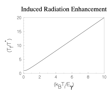
Figure 1: If $T_{i}$ represents the initial cavity mode temperature and $T^{*}$ represents the noise temperature of the pair radiated photons, then the final temperature $T_{f}$ of the of the cavity mode is enhanced (over and above $T^{*})$ via the initial photon population. The resulting radiation enhancement is plotted for photons with energy $E_{\gamma}=\hbar\Omega_{0}$.

The probability of such a photon pair creation event defines a photon pair creation noise temperature $T^{*}$ induced by the time varying frequency via

$$R=|\rho|^{2}=e^{-\hbar\Omega_{0}/k_{B}T^{*}}.$$ (27)

The mean number $\bar{N}$ of photons which would be radiated from the vacuum by a time varying frequency modulation $\Omega(t)$ obeys a formal Planck law

$$\bar{N}=\frac{R}{1-R}=\frac{1}{e^{\hbar\Omega_{0}/k_{B}T^{*}}-1}\ .$$ (28)

Suppose (for example) that a microwave cavity is initially in thermal equilibrium at temperature $T_{i}$. The mean number of initial microwave photons in a given normal mode is then given by

$$N_{i}=\frac{1}{e^{\hbar\Omega_{0}/k_{B}T_{i}}-1}\ .$$ (29)

After a sequence of frequency modulation pulses the mean number of final photons in the cavity mode is

$$N_{f}=(2\bar{N}+1)N_{i}+\bar{N}=N_{i}\coth\left(\frac{\hbar\Omega_{0}}{2k_{B}T^{*}}\right)+\frac{1}{e^{\hbar\Omega_{0}/k_{B}T^{*}}-1}\ .$$ (30)

Note that the existence of an initial number of photons $N_{i}$ in the cavity mode makes larger the final number of of photons

$$N_{f}=\frac{1}{e^{\hbar\Omega_{0}/k_{B}T_{f}}-1}$$ (31)

via the induced radiation of additional photon pairs. If the microwave frequency large margin inequality

$$\hbar\Omega_{0}\ll k_{B}T^{*}$$ (32)

holds true, then Eqs.(28) - (32) imply an approximate law for the final cavity mode noise temperature is given by

$$T_{f}\approx T^{*}\coth\left(\frac{\hbar\Omega_{0}}{2k_{B}T_{i}}\right).$$ (33)

The resulting enhancement $(T_{f}/T^{*})$ is plotted in Fig.1. The dynamical Casimir effect for frequency modulation pulses is thereby described in terms of the amount of heat that raises the temperature $T_{i}\to T_{f}$ of the microwave cavity.

6 Periodic Frequency Modulations

For periodic modulations in the frequency one must examine[12] the differential equation

$$\ddot{\phi}(t)+\Omega^{2}(t)\phi(t)=0,$$

$$\Omega^{2}(t)=\Omega_{0}^{2}+\nu^{2}(t),$$

$$\nu(t+\tau)=\nu(t).$$ (34)

From a mathematical viewpoint, Eq.(34) has been well studied. If $\nu(t)$ can be represented as a non-overlapping pulse sequence of the form

$$\nu(t)=\sum_{n=-\infty}^{\infty}\varpi(t-n\tau),$$ (35)

then the transmission problem for a single pulse,

$$\ddot{\phi}_{1}(t)+\{\Omega_{0}^{2}+\varpi^{2}(t)\}\phi_{1}(t)=0,$$ (36)

yields a complete solution to the general problem. In particular we examine the two photon creation problem as in Eq.(26); i.e.

$$\phi_{1}(t\to\infty)=e^{i\Omega_{0}t}+\rho_{1}e^{-i\Omega_{0}t},$$

$$\phi_{1}(t\to-\infty)=\sigma_{1}e^{i\Omega_{0}t},$$

$$|\rho_{1}|^{2}+|\sigma_{1}|^{2}=R_{1}+P_{1}=1,$$

$$\sigma_{1}=\sqrt{P_{1}}\ e^{-i\Theta_{1}}.$$ (37)

Employing the characteristic function

$$\mu(\Omega_{0})=\frac{\cos(\Omega_{0}\tau+\Theta_{1}(\Omega_{0}))}{\sqrt{P_{1}(\Omega_{0})}},$$ (38)

one may study the stability problem for the dynamic Casimir effect. For periodic frequency modulations there are two cases of interest:

Case I: Stable Motions $-1<\mu(\Omega_{0})<+1$

$$\mu(\Omega_{0})=\cos(\Omega\tau)$$

$$\phi_{\pm}(t+\tau)=e^{\pm i\Omega t}\phi_{\pm}(t).$$ (39)

Case II: Unstable Motions $\mu(\Omega_{0})>+1$ or $\mu(\Omega_{0})<-1$

$$\mu(\Omega_{0})=\cosh(\gamma\tau)\ \ {\rm or}\ \ \mu(\Omega_{0})=-\cosh(\gamma\tau)$$

$$\phi_{\pm}(t+\tau)=e^{\pm\gamma t}\phi_{\pm}(t).$$ (40)

In the unstable regime, $2\gamma$ represents the number of cavity photons being produced per unit time. If the cavity mode has a high quality factor $Q\gg 1$, then photons are also absorbed at a rate $(\Omega_{0}/Q)$. The net photon production rate in this approximation would then be

$$\Gamma_{1}\simeq\left(2\gamma-\frac{\Omega_{0}}{Q}\right),$$ (41)

and the theoretical noise temperature after $n_{p}$ pulses would be

$$k_{B}T_{1}^{*}\approx\hbar\Omega_{0}\exp(n_{p}\tau\Gamma_{1}).$$ (42)

As an example, let us suppose a sequence of rectangular pulse sequences of the form

$$\Omega(t)=\Omega_{0}\ \ \ {\rm if}\ \ \ t_{0}+n\tau<t<t_{0}+(n+1/2)\tau,$$

$$\Omega(t)=(1+\alpha)\Omega_{0}\ \ \ {\rm if}\ \ \ t_{0}+(n+1/2)\tau<t<t_{0}+(n+1)\tau,$$ (43)

wherein $n=1,2,\ldots,n_{p}$. The estimate

$$\exp(n_{p}\tau\Gamma_{1})\sim\exp(n_{p}\alpha/2)\ \ \ {\rm for}\ \ \ 1\gg\alpha\gg(\Omega_{0}\tau)/Q$$ (44)

is not unreasonable.

The exponential temperature instability for high quality cavity modes, i.e. $\Gamma_{1}>0$ in Eqs.(41) - (44), would be sufficient for large $n_{p}$ to melt the cavity. No microwave oven works that efficiently even if the dynamic Casimir effect were employed for exactly that purpose. The one loop photon approximation is evidently at fault and higher loops (non-linear processes) must be invoked for the noise temperature of the mode to be theoretically stable as would be laboratory microwave cavities.

7 Microwave Intensity Stability

The stability of the microwave cavity is due to the fact that the modulation is induced by a pump which supplies the energy of the induced cavity radiation. One may define a pump coordinate $\eta$ which in general is a quantum mechanical operator. In principle, one might mechanically vibrate a wall in the cavity in which case $\eta$ would be proportional to a mechanical displacement. In practice, changing the frequency by electronic means may well be more efficient. Be that as it may, let us define the coordinate so that

$$\left<\eta(t)\right>=\frac{\nu^{2}(t)}{\Omega_{0}^{2}}\ ,$$ (45)

wherein the quantities on the right hand side of Eq.(45) are given in Eq.(34).

If the quantum pump coordinate exhibits stationary fluctuations

$$\Delta\eta=\eta-\left<\eta\right>$$ (46)

with quantum noise

$$\frac{1}{2}\left<\Delta\eta(t)\Delta\eta(t^{\prime})+\Delta\eta(t^{\prime})\Delta\eta(t)\right>=\int_{-\infty}^{\infty}\bar{S}_{\eta}(\omega)e^{-i\omega(t-t^{\prime})}d\omega,$$ (47)

then two photon absorption and two photon emission processes are described by the additional noise Hamiltonian

$$\Delta H=\frac{1}{4}\hbar\Omega_{0}\left(a^{\dagger}a^{\dagger}+aa\right)\Delta\eta.$$ (48)

The usual mode photon creation and destruction operators are $a^{\dagger}$ and $a$, respectively. When the Hamiltonian in Eq.(48) is taken to second order in perturbation theory, the resulting energies involve four boson processes and thereby introduces multi-photon loop processes.

With the pump coordinate positive and negative frequency spectral functions

$$\left<\Delta\eta(t)\Delta\eta(t^{\prime})\right>=\int_{-\infty}^{\infty}S_{\eta}^{+}(\omega)e^{-i\omega(t-t^{\prime})}d\omega,$$

$$\left<\Delta\eta(t^{\prime})\Delta\eta(t)\right>=\int_{-\infty}^{\infty}S_{\eta}^{+}(\omega)e^{-i\omega(t-t^{\prime})}d\omega,$$ (49)

the two photon Fermi golden rule transition rates which follow from Eqs.(48) and (49) read

$$\Gamma^{+}(n\to n-2)=\frac{\pi\Omega_{0}^{2}}{8}S_{\eta}^{+}(\omega=2\Omega_{0})n(n-1),$$

$$\Gamma^{-}(n-2\to n)=\frac{\pi\Omega_{0}^{2}}{8}S_{\eta}^{-}(\omega=2\Omega_{0})n(n-1).$$ (50)

The pump coordinate also has a noise temperature $T_{\eta}$ may be defined via

$$S_{\eta}^{-}(2\Omega_{0})=e^{-2\hbar\Omega_{0}/k_{B}T_{\eta}}S_{\eta}^{+}(2\Omega_{0}).$$ (51)

If there a many photons in the mode, then the net rate of photon absorption is given by

$$\Gamma_{absorption}\simeq\left(\frac{\pi\Omega_{0}^{2}\bar{S}_{\eta}(\omega=2\Omega_{0})}{2}\right)\tanh\left(\frac{\hbar\Omega_{0}}{k_{B}T_{\eta}}\right)n^{2}.$$ (52)

On the other hand the frequency modulation produces photons at a rate

$$\Gamma_{emmision}\simeq 2\gamma n\ \ \ {\rm where}\ \ \ n\gg 1\ ,$$ (53)

and $\gamma$ is defined in Eq.(40). We may now state the central result of this section:

Theorem 2: If the pump coordinate pushes the cavity mode into a modulation dynamic Casimir instability, then the quantum noise will stabilize the cavity mode according to the equation

$$\frac{dn}{dt}=2(\gamma n-\tilde{\gamma}n^{2}),$$

$$\tilde{\gamma}={\pi\Omega_{0}^{2}\bar{S}_{\eta}(\omega=2\Omega_{0})}\tanh\left(\frac{\hbar\Omega_{0}}{k_{B}T_{\eta}}\right).$$ (54)

The cavity photon occupation number will then saturate according to

$$\bar{n}_{saturate}=\frac{\gamma}{\pi\Omega_{0}^{2}\bar{S}_{\eta}(\omega=2\Omega_{0})}\coth\left(\frac{\hbar\Omega_{0}}{k_{B}T_{\eta}}\right).$$ (55)

More simply, with the response function

$$\chi(\zeta)=\frac{i}{\hbar}\int_{0}^{\infty}\left<\left[\eta(t),\eta(0)\right]\right>e^{i\zeta t}dt,$$ (56)

the fluctuation dissipation theorem

$$\bar{S}_{\eta}(\omega)=\left(\frac{\hbar}{2\pi}\right)\coth\left(\frac{\hbar\omega}{2k_{B}T_{\eta}}\right){\Im m}\chi(\omega+i0^{+}).$$ (57)

together with Eqs.(55) and (56) reads

$$\bar{n}_{saturate}=\frac{2\gamma}{\Omega_{0}^{2}[\hbar{\Im m}\chi(2\Omega_{0}+i0^{+})]}.$$ (58)

The relation time $\tau^{\dagger}$ for the parameter $\eta$ may be conventionally defined[15] by

$$\chi(0)\tau^{\dagger}=\lim_{\omega\to 0}\frac{{\Im}m\chi(\omega+i0^{+})}{\omega}$$ (59)

so that

$$\bar{n}_{saturate}\approx\frac{\gamma}{\Omega_{0}^{3}\tau^{\dagger}\hbar\chi(0)}.$$ (60)

Eq.(60) is our final answer for the number of final photons at saturation.

8 A Numerical Example

In order to make our final answer less abstract, let us consider a proposed[14] experiment. In that proposal, the parameter $\eta$ describes the metallic conductivity in a semiconductor plate due to a laser beam inducing particle hole pairs. If we let $\tau_{R}$ represent the recombination time taken to annihilate a particle hole pair in the semiconductor and let $\omega_{L}$ represent the laser frequency, then we estimate that

$$\frac{1}{\tau^{\dagger}}\sim\frac{\hbar\omega_{L}\chi(0)}{\tau_{R}}$$ (61)

which implies

$$\bar{n}_{saturate}\sim\left(\frac{\gamma}{\Omega_{0}}\right)\left(\frac{1}{\Omega_{0}\tau_{R}}\right)\left(\frac{\omega_{L}}{\Omega_{0}}\right).$$ (62)

The following estimates are reasonable for the proposal[14]:

$$\left(\frac{\gamma}{\Omega_{0}}\right)\sim 0.05,$$

$$\left(\frac{1}{\Omega_{0}\tau_{R}}\right)\sim 10,$$

$$\left(\frac{\omega_{L}}{\Omega_{0}}\right)\sim 2\times 10^{5},$$

$$\bar{n}_{saturate}\sim 10^{5}\ {\rm microwave\ photons.}$$ (63)

9 Conclusion

We have explored the concept of induced instabilities in both the static and dynamic Casimir effects. For the static case, large quantum electrodynamic collective Lamb shifts in condensed matter can induce a phase transition requiring a new equilibrium position of the microwave oscillator coordinates. In particular, when at the quadratic level and oscillator goes unstable, quartic terms can be invoked to make the system stable. For the dynamic case, even if the frequency shifts are small, perfect periodicity in modulation pulses can build up to exponentially large proportions again leading to an instability. Again dynamic quartic terms can stabilize the cavity modes. The basic principle involved is that the shifted frequencies themselves must undergo fluctuations. Given the noise fluctuations in the pump coordinate, the final saturation temperature of the microwave cavity can be computed from Eq.(60).

References

[1]
H.B.G. Casimir and D. Polder, Phys. Rev.73, 360 (1948).
[2]
H.B.G. Casimir Proc. K. Ned. Akad. Wet.60, 793 (1948).
[3]
M. Bordag, U. Mohideen, and V. M. Mostepanenko,
Phys. Rep.205, 353 (2001).
[4]
K. A. Milton, “The Casimir Effect”, World Scientific,
River Edge, (2001).
[5]
I.E. Dzyaloshinski, E.M. Lifshitz and L.P. Pitayevski,
Sov. Phys. JETP10, 161 (1960).
[6]
I.E. Dzyaloshinski, E.M. Lifshitz and L.P. Pitayevski,
Adv. Phys.10, 165 (1961).