Exploring super-radiant phase transitions via coherent control of a multi-qubit–cavity system

Abstract

We propose the use of coherent control of a multi-qubit–cavity QED system in order to explore novel phase transition phenomena in a general class of multi-qubit–cavity systems. In addition to atomic systems, the associated super-radiant phase transitions should be observable in a variety of solid-state experimental systems, including the technologically important case of interacting quantum dots coupled to an optical cavity mode.

,

1 Introduction

There is much current interest in the use of coherent control in order to generate novel matter-radiation states in cavity QED and atom-optics systems [1]. In addition, the field of cavity QED has caught the interest of workers in the field of solid-state nanostructures, since effective two-level systems can be fabricated using semiconductor quantum dots, organic molecules and even naturally-occuring biological systems such as the photosynthetic complexes LHI and LHII and in biological imaging setups involving FRET (Fluoresence Resonance Energy Transfer) [2]. Such nanostructure systems could then be embedded in optical cavities or their equivalent, such as in the gap of a photonic band-gap material [3]. We refer to Ref. [4] for a discussion of the size and energy-gaps of the artificial nanostructure systems which can currently be fabricated experimentally.

In a parallel development, phase transitions in quantum systems are currently attracting much attention within the solid-state, atomic and quantum information communities [5, 6, 7, 8]. Most of the focus within the solid-state community has been on phase transitions in electronic systems such as low-dimensional magnets [5, 6] while in atomic physics there has been much interest in phase transitions in cold atom gases and in atoms coupled to a cavity. In particular, a second-order phase transition, from normal to superradiant, is known to arise in the Dicke model which considers $N$ two-state atoms (i.e. ‘spins’ or ‘qubits’ [7, 8]) coupled to an electromagnetic field (i.e. bosonic cavity mode) [9, 10, 11]. The Dicke model itself has been studied within the atomic physics community for fifty years, but has recently caught the attention of solid-state physicists working on arrays of quantum dots, Josephson junctions, and magnetoplasmas [13]. Its extension to quantum chaos [14], quantum information [15] and other exactly solvable models has also been considered recently [16]. It has also been conjectured that superradiance could be used as a mechanism for quantum teleportation [17].

Here we extend our discussion in Ref. [18] on the exploration of novel phase transitions in atom-radiation systems exploiting the current levels of experimental expertise in the area of coherent control. The corresponding experimental set-up can be a cavity-QED, atom-optics, or nanostructure-optics system, whose energy gaps and interactions are tailored to be the required generalization of the well-known Dicke model [11]. We show that, according to the values of these control parameters, the phase transitions be driven to become first-order.

2 The Model

The well-known Dicke model from atom-optics ignores interactions between the constituent two-level systems or ‘spins’ [11]. In atomic systems where each ‘spin’ is an atom, this is arguably an acceptable approximation if the atoms are neutral and the atom-atom separation $d\gg a$ where $a$ is the atomic diameter. However there are several reasons why this approximation is unlikely to be valid in typical solid-state systems. First, the ‘spin’ can be represented by any nanostructure (e.g. quantum dot) possessing two well-defined energy levels, yet such nanostructures are not typically neutral. Hence there will in general be a short-ranged (due to screening) electrostatic interaction between neighbouring nanostructures. Second, even if each nanostructure is neutral, the typical separation distance $d$ between fabricated and self-organised nanostructures is typically the same as the size of the nanostructure itself. Hence neutral systems such as excitonic quantum dots will still have a significant interaction between nearest neighbors [19].

Motivated by the experimental relevance of ‘spin–spin’ interactions, we introduce and analyze a generalised Dicke Hamiltonian which is relevant to current experimental setups in both the solid-state and atomic communities [20]. We show that the presence of transverse spin–spin coupling terms, leads to novel first-order phase transitions associated with super-radiance in the bosonic cavity field. A technologically important example within the solid-state community would be an array of quantum dots coupled to an optical mode. This mode could arise from an optical cavity, or a defect mode in a photonic band gap material [20]. However we emphasise that the $N$ ‘spins’ may correspond to any two-level system, including superconducting qubits and atoms [13, 20]. The bosonic field is then any field to which the corresponding spins couple [13, 20]. Apart from the experimental prediction of novel phase transitions, our work also provides an interesting generalisation of the well-known Dicke model.

The method of solution that we present here is in fact valid for a wider class of Hamiltonians incorporating spin–spin and spin–boson interactions [21]. We follow the method of Wang and Hioe [11], whose results also proved to be valid for a wider class of Dicke Hamiltonians. We focus on the simple example of the Dicke Hamiltonian with an additional spin–spin interaction in the $y$ direction.

$$H = a^{\dagger}a+\sum_{j=1}^{N}\left\{\frac{\lambda}{2\sqrt{N}}(a+a^{\dagger})(\sigma^{+}_{j}+\sigma^{-}_{j})+\frac{\epsilon}{2}\sigma^{Z}_{j}-J\sigma^{Y}_{j}\cdot\sigma^{Y}_{j+1}\right\}$$ (1)

$$= a^{\dagger}a+\sum_{j=1}^{N}\left\{\frac{\lambda}{\sqrt{N}}(a+a^{\dagger})\sigma^{X}_{j}+\frac{\epsilon}{2}\sigma^{Z}_{j}-J\sigma^{Y}_{j}\cdot\sigma^{Y}_{j+1}\right\}\ .$$ (2)

Following the discussion above, the experimental spin–spin interactions are likely to be short-ranged and hence only nearest-neighbor interactions are included in $H$. The operators in Eqs. 1 and 2 have their usual, standard meanings.

3 Results

To obtain the thermodynamical properties of the system, we first introduce the Glauber coherent states $|\alpha\rangle$ of the field [12] where $a|\alpha\rangle=\alpha|\alpha\rangle$, $\langle\alpha|a^{\dagger}=\langle\alpha|\alpha^{*}$. The coherent states are complete, $\int\frac{d^{2}\alpha}{\pi}|\alpha\rangle\langle\alpha|=1$. In this basis, we may write the canonical partition function as:

$$Z(N,T)=\sum_{\bf s}\int\frac{d^{2}\alpha}{\pi}\langle{\bf s}|\langle\alpha|e^{-\beta H}|\alpha\rangle|{\bf s}\rangle$$ (3)

As in Ref. [11], we adopt the following assumptions:

1. $a/\sqrt{N}$ and $a^{\dagger}/\sqrt{N}$ exist as $N\rightarrow\infty$;

2. $\lim_{N\rightarrow\infty}\lim_{R\rightarrow\infty}\sum_{r=0}^{R}\frac{(-\beta H_{N})^{r}}{r!}$ can be interchanged

We then find

$$Z(N,T)=\int\frac{d^{2}\alpha}{\pi}e^{-\beta|\alpha|^{2}}{\rm Tr}e^{-\beta H^{\prime}}$$ (4)

where

$$H^{\prime}=\sum_{j=1}^{N}\left\{\frac{2\lambda{\rm Re}(\alpha)}{\sqrt{N}}\sigma^{X}_{j}+\frac{\epsilon}{2}\sigma^{Z}_{j}-J\sigma^{Y}_{j}\cdot\sigma^{Y}_{j+1}\right\}.$$ (5)

We first rotate about the $y$-axis to give

$$H^{\prime}=-J\sum_{j=1}^{N}\left\{\sqrt{\left(\frac{2\lambda{\rm Re}(\alpha)}{J\sqrt{N}}\right)^{2}+\left(\frac{\epsilon}{2J}\right)^{2}}\sigma^{Z^{\prime}}_{j}+\sigma^{Y}_{j}\cdot\sigma^{Y}_{j+1}\right\}.$$ (6)

We note here that the resulting hamiltonian is of the type of an Ising hamiltonian with a transverse field, and it exhibits a divergence in concurrence at its quantum phase transition (see, e.g., [7]). This particular model is instrumental in understanding the nature of coherence in quantum systems. Going back to the calculations, we may now diagonalise $H^{\prime}$ by performing a Jordan-Wigner transformation, passing into momentum-space and then performing a Bogoliubov transformation (see, for example, Ref. [6]). We then have, in terms of momentum-space fermion operators $\gamma_{k}$, the diagonalised $H^{\prime}$:

$$H^{\prime}=\sum_{k=1}^{N}\xi_{k}(\alpha)(\gamma_{k}^{\dagger}\gamma_{k}-\frac{1}{2})$$ (7)

with

$$\xi_{k}(\alpha) = 2J\sqrt{1+(g(\alpha))^{2}-2g(\alpha)}$$ (8)

$$g(\alpha) = \sqrt{\left(\frac{2\lambda{\rm Re}(\alpha)}{J\sqrt{N}}\right)^{2}+\left(\frac{\epsilon}{2J}\right)^{2}}\ .$$ (9)

We may then write

$$H^{\prime}=\sum_{k=1}^{N}H_{k}$$ (10)

where

$$H_{k}=\xi_{k}(\alpha)(\gamma_{k}^{\dagger}\gamma_{k}-\frac{1}{2}).$$ (11)

From the transformation, we may associate the spin-up state with an empty orbit on the site and a spin-down state with an occupied orbital. Using the commutation relations for the $\gamma_{k}$ and the fact that $\gamma_{k}|0\rangle=0$ (see, for example, Ref. [6]), we obtain

$$Z(N,T)=\int\frac{d^{2}\alpha}{\pi}e^{-\beta|\alpha|^{2}}\prod_{k=1}^{N}\{e^{-\frac{\beta}{2}\xi_{k}(\alpha)}+e^{\frac{\beta}{2}\xi_{k}(\alpha)}\}.$$ (12)

Writing $d^{2}\alpha=d{\rm Re}(\alpha)d{\rm Im}(\alpha)$, $w={\rm Re}(\alpha)$ and integrating out ${\rm Im}(\alpha)$ we obtain

$$Z(N,T)=\frac{1}{\sqrt{\beta}{\pi}}\int dwe^{-\beta w^{2}+\sum_{k=1}^{N}\left\{\log\left[\cosh\left(\frac{\beta}{2}\xi_{k}(x)\right)\right]+\log(2)\right\}}\ .$$ (13)

We now let $x=w/\sqrt{N}$. Writing $\sum_{k=1}^{N}$ as $\frac{N}{2\pi}\int_{0}^{2\pi}dk$, yields

$$Z(N,T)=\sqrt{\frac{N}{\beta\pi}}\int_{-\infty}^{\infty}dx\left\{e^{-\beta x^{2}+I(x)}\right\}^{N}$$ (14)

where

$$I(x) = \frac{1}{2\pi}\int_{0}^{2\pi}dk\left\{\log\left[\cosh\left(\frac{\beta}{2}\xi_{k}(x)\right)\right]+\log(2)\right\}$$ (15)

and

$$\xi_{k}(x)=2J\sqrt{1+(g(x))^{2}-2g(x)\cos k}\ .$$ (16)

From here on, we omit the $\log(2)$ term in $I(x)$ since it only contributes an overall factor to $Z(N,T)$.

Laplace’s method now tells us that

$$Z(N,T)\propto\max_{-\infty\leq x\leq\infty}\exp\left\{N[-\beta x^{2}+I(x)]\right\}.$$ (17)

Denoting $[-\beta x^{2}+I(x)]$ by $\Omega(x)$, we recall that the super-radiant phase corresponds to $\Omega(x)$ having its maximum at a non-zero $x$ [11]. If there is no transverse field, i.e., if $J=0$, and the temperature is fixed, then the maximum of $\Omega(x)$ will split continuously into two maxima symmetric about the origin as $\lambda^{2}$ increases. Hence the process is a continuous phase transition.

However the case of non-zero $J$ is qualitatively different from $J=0$. As a result of the frustration induced by the tranverse nearest-neighbour couplings, there are regions where the super-radiant phase transition becomes first-order. Hence the system’s phase transition can be driven to become first-order by suitable adjustment of the nearest-neighbour couplings. This phenomenon of first-order phase transitions is revealed by considering the functional shape of $\Omega(x)$, as shown in Fig. 1.

Figure 2 shows the value of $x$ that maximises $\Omega(x)$ at fixed $\epsilon$ and two different values of $J$. From the two lines, we can see that the spin–spin coupling actually acts to inhibit the phase transition. As we increase $J$ from $0.8$ to $1.0$ we can see that the value to which we have to increase $\lambda$ to induce a phase transition is higher.

Figure 3 plots the maximiser of $\Omega(x)$ with $\lambda$ fixed at a value of 1.3. For small $J$, the local (non-zero) maximum of $\Omega(x)$ converges to zero as we increase $\epsilon$ and the system is no longer super-radiant. This is no longer the case if $J$ is increased. In this case, $\Omega(x)$ has a global maximum when $\epsilon$ is small; however as $\epsilon$ increases, the non-zero local maxima becomes dominant and as a result a first-order phase transition occurs. We note that the barriers between the wells are infinite in the thermodynamic limit, hence we expect that the sub-radiant state is metastable as $\epsilon$ increases. This observation also suggests the phenomenon of hysteresis, which awaits experimental validation.

In Fig. 4 we consider the order parameter of the transition, $\langle\frac{a^{\dagger}a}{N}\rangle$. Following the same method as above, we may calculate this to be equivalent to $x^{2}$ with an additional $\frac{1}{2\beta}$ term that comes from the imaginary part of the coherent states of the radiation field [22]. We can see from the figure that as we lower $\beta$ we drive the system first through a first order phase transition and then through a continuous phase transition. Thus we are able to achieve both a first and second order phase transition by varying the one parameter, $\beta$.

4 Conclusion

In conclusion, we have shown that the experimentally relevant spin-spin interaction in the Dicke model transforms it into an Ising-hamiltonian with a photon-field dependent transverse field, which allows for an existence of both first-order and second-order phase transitions as parameters vary. Our results highlight the importance of spin-spin coupling terms in spin-boson systems and opens up the possibility of coherently controlling the competition between the sub-radiant and super-radiant states in experimental atom-radiation systems [21].

References

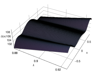
Figure 1: Demonstration as to what the function $\Omega(x)$ looks like across a first-order phase transition as $\lambda$ and $x$ are varied. Here $J=1.0$, $\epsilon=1.1$ and $\beta=100.0$.

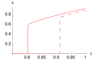
Figure 2: The value of $x$ at which there is a maximum in $\Omega(x)$ as $\lambda$ increases, for $J=1.0$ (dashed line) and $J=0.8$ (solid line). In both cases $\epsilon=1.1$ and $\beta=100$.

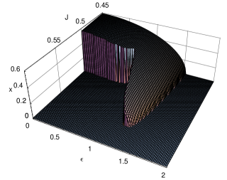
Figure 3: The maximiser of $\Omega$ shown as a function of $J$ and $\epsilon$. Here $\lambda=1.3$ and $\beta=100$.

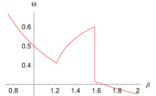
Figure 4: Plot of the order parameter, $\Theta=\langle\frac{a^{\dagger}a}{N}\rangle$, for the phase transition with $\lambda=0.9$, $J=1.0$ and $\epsilon=1.1$.

References

- [1] See, for example, A. Olaya-Castro, N. F. Johnson and L Quiroga, Phys. Rev. A 70, 020301(R) (2004); J. Opt. B: Quantum Semiclass. Opt. 6, S730 (2004); Phys. Rev. Lett., in press (2005).
- [2] A.J. Berglund, A.C. Doherty and H. Mabuchi, Phys. Rev. Lett. 89, 068101 (2002); J. Gilmore and R.H. McKenzie, cond-mat/0401444; A. Olaya-Castro, C.F. Lee and N.F. Johnson, in preparation (2005).
- [3] P.M. Hui and N.F. Johnson, Solid State Physics, Vol. 49, edited by H. Ehrenreich and F. Spaepen (Academic Press, New York, 1995).
- [4] A. Olaya-Castro and N. F. Johnson, Handbook of Theoretical and Computational Nanotechnology, in press (2005); quant-ph/0406133.
- [5] L.P. Kadanoff, Statistical Physics (World Scientific, Singapore, 2000).
- [6] S. Sachdev, Quantum Phase Transitions (Cambridge University Press, Cambridge, 1999).
- [7] T.J. Osborne and M.A. Nielsen, Phys. Rev. A 66, 032110 (2002); R. Somma, G. Ortiz, H. Barnum, E. Knill, and L. Viola, quant-ph/0403035.
- [8] M.A. Nielsen and I.L. Chuang, Quantum Computation and Quantum Information (Cambridge University Press, Cambridge, 2002).
- [9] R.H. Dicke, Phys. Rev. 170, 379 (1954).
- [10] K. Hepp and E.H. Lieb, Ann. Phys. (N.Y.) 76, 360 (1973).
- [11] Y.K. Wang and F.T. Hioe, Phys. Rev. A 7, 831 (1973); F.T. Hioe, Phys. Rev. A 8, 1440 (1973).
- [12] R. Glauber, Phys. Rev. 131, 2766 (1963).
- [13] T. Vorrath and T. Brandes, Phys. Rev. B 68, 035309 (2003); W.A. Al-Saidi and D. Stroud, Phys. Rev. B 65, 224512 (2002); X. Zou, K. Pahlke and W. Mathis, quant-ph/0201011; S. Raghavan, H. Pu, P. Meystre and N.P. Bigelow, cond-mat/0010140; N. Nayak, A.S. Majumdar and V. Bartzis, J. Nonlinear Optics 24, 319 (2000); T. Brandes, J. Inoue and A. Shimizu, cond-mat/9908448 and cond-mat/9908447.
- [14] C. Emary and T. Brandes, Phys. Rev. Lett. 90, 044101 (2003); Phys. Rev. E 67, 066203 (2003).
- [15] N. Lambert, C. Emary and T. Brandes, Phys. Rev. Lett. 92, 073602 (2004); S. Schneider and G.J. Milburn, quant-ph/0112042; G. Ramon, C. Brif and A. Mann, Phys. Rev. A 58, 2506 (1998); A. Messikh, Z. Ficek and M.R.B. Wahiddin, quant-ph/0303100.
- [16] C. Emary and T. Brandes, quant-ph/0401029; S. Mancini, P. Tombesi and V.I. Man’ko, quant-ph/9806034.
- [17] Y.N. Chen et al., cond-mat/0502412.
- [18] C.F. Lee and N.F. Johnson, Phys. Rev. Lett. 93, 083001 (2004).
- [19] L. Quiroga and N.F. Johnson, Phys. Rev. Lett. 83, 2270 (1999); J.H. Reina, L. Quiroga and N.F. Johnson, Phys. Rev. A 62, 012305 (2000).
- [20] E. Hagley et al., Phys. Rev. Lett. 79, 1 (1997); A. Rauschenbeutel et al., Science 288, 2024 (2000); A. Imamoglu et al., Phys. Rev. Lett. 83, 4204 (1999); S.M. Dutra, P.L. Knight and H. Moya-Cessa, Phys. Rev. A 49, 1993 (1994); Y. Yamamoto and R. Slusher, Physics Today, June (1993), p. 66; D.K. Young, L. Zhang, D.D. Awschalom and E.L. Hu, Phys. Rev. B 66, 081307 (2002); G.S. Solomon, M. Pelton and Y. Yamamoto, Phys. Rev. Lett. 86, 3903 (2001); B. Moller, M.V. Artemyev and U. Woggon, Appl. Phys. Lett. 80, 3253 (2002); N. F. Johnson, J. Phys. Condens. Matter 7, 965 (1995).
- [21] C.F. Lee, T.C. Jarrett and N.F. Johnson, unpublished.
- [22] G.C. Duncan, Phys. Rev. A 9, 418 (1974).