Quantum Zeno and anti-Zeno effects in an Unstable System with Two Bound State

Abstract

We analyze the experimental observations reported by Fischer et al [in Phys. Rev. Lett. 87, 040402 (2001)] by considering a system of coupled unstable bound quantum states $\mathinner{|{A}\rangle}$ and $\mathinner{|{B}\rangle}$. The state $\mathinner{|{B}\rangle}$ is coupled to a set of continuum states $\mathinner{|{C\Theta(\omega)}\rangle}$. We investigate the time evolution of $\mathinner{|{A}\rangle}$ when it decays into $\mathinner{|{C\Theta(\omega)}\rangle}$ via $\mathinner{|{B}\rangle}$, and find that frequent measurements on $\mathinner{|{A}\rangle}$ leads to both the quantum Zeno effect and the anti-Zeno effects depending on the frequency of measurements. We show that it is the presence of $\mathinner{|{B}\rangle}$ which allows for the anti-Zeno effect.

I Introduction

The quantum Zeno effect, first predicted by Misra and Sudarshan Misra and Sudarshan (1977); Chiu et al. (1977), is the hindrance of the time evolution of a quantum state when frequent measurements are performed on it. In the limit of continuous measurement the time evolution of the state, in principle, completely stops. The seminal paper by Misra and Sudarshan proves the existence of an operator corresponding to continuous measurement belonging to the Hilbert space of a generic quantum system. More recently, several authors have suggested that the opposite of quantum Zeno effect may also be true Kaulakys and Gontis (1997); Kofman and Kurizki (2000); Facchi et al. (2001). That is, frequent measurements can be used to accelerate the decay of an unstable state. This effect is known as the anti-Zeno effect or the inverse Zeno effect. The original formulation of the quantum Zeno effect treated the measurement process as an idealized von-Neumann type; that is an instantaneous event that induces discontinuous changes in the measured system. The anti-Zeno effect was first identified as a possibility when measurement processes that take a finite amount of time were considered. This led to the suggestion by several authors that the anti-Zeno effect should be observed more often in physical systems than the quantum Zeno effect.

Experimental evidence supporting the quantum Zeno effect in particle physics experiments was first pointed out by Valanju et al Valanju et al. (1980); Valanju (1980). Direct experimental observation of the quantum Zeno effect was obtained by Itano et al Itano et al. (1990) in a three-level oscillating system. Recently, in a set of experiments Fischer, Gutierrez-Medina, and Raizen observed, for the first time, both the quantum Zeno effect and the anti-Zeno effect in an unstable quantum mechanical system Fischer et al. (2001). In this Letter we present a simple model that reproduces all of the important results of this experiment.

This Letter is organized as follows: We briefly describe the experiment by Fischer et al in section II. In section III, we present a simplified model of the system studied experimentally in Fischer et al. (2001). The model is exactly solvable and the time dependence of the survival probability of the initial unstable state can be analytically calculated. In section IV, we show that the solutions reproduce all the important features of the experimental system. On the basis of our model we argue that the anti-Zeno effect is observed because of the presence of more than one unstable bound states in the system. Our conclusions are in section V.

II Description of the Experiment

In the experiment by Fischer et al Fischer et al. (2001), sodium atoms were placed in a classical magneto-optical trap that could be moved in space. The motional states of the atoms in the trap were studied. Initially, the atoms were placed in the “ground” state of the moving trap so that they remained inside the trap. The stable bound states occupied by the atoms in the trap are made unstable by accelerating the atoms along with the trap at different rates. By tuning the acceleration appropriate conditions are created for the atoms to quantum mechanically tunnel through the barrier into the continuum of available free-particle states. The number of atoms that tunneled out of the bound state inside the trap as a function of time was estimated at the end of the experiment by recording the spatial distribution of the atoms. Since the trap was accelerated throughout the experiment, atoms that spent more time in the and trap had higher velocities and they moved farther in unit time. So by taking a snap-shot of the spatial distribution of all the atoms at the end of the experiment the time at which each one of them tunneled out of the trap can be estimated.

To obtain the Zeno and the anti-Zeno effects, the tunneling of the atoms out of the trap has to be interrupted by a measurement that estimates the number of atoms still inside the trap. Such a measurement was implemented in the experiment by abruptly changing the acceleration of the trap so that tunneling from the ground state is temporarily halted. These interruption periods were long enough ($40\mu s$) to separate out the atoms that tunnel out before and after each interruption into resolvable groups. By measuring the number of atoms in each group and knowing the total number of atoms that were initially in the trap, the number of atoms in the trap at the beginning of each interruption period was estimated. Using this data, the time dependence of the survival probability of the bound motional states of an atom was reconstructed. Their observations are summarized in Fig. 1.

The frequency with which interruption periods were applied determined whether the Zeno or anti-Zeno effects were obtained. Repeatedly interrupting the system once every micro-second led to the quantum Zeno effect. With an interruption rate of $5\mu s$ the anti-Zeno effect was obtained.

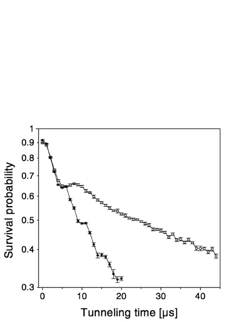
Figure 1: On the left, the lower line is the “unmeasured” decay curve corresponding to the case where the trapped atoms are accelerated with no interruptions so that tunneling out of the trap is always present. The upper line corresponds to the case where the tunneling is interrupted every 1 $\mu$s leading to the quantum Zeno effect. On the right, the upper line is the “unmeasured” decay and the lower line corresponds to interruptions every 5 $\mu$s leading to the anti-Zeno effect in the experiment by Fischer et al.

In Fig1, the zero slope for the survival probability at $t=0$ is expected for the time evolution of a generic unstable quantum state on the basis of the analyticity of the survival probability and its time reversal symmetry Winter (1961). This non-exponential behavior at short times leads to the quantum Zeno effect.

The shape of survival probability as a function of time of the “unmeasured system” has an inflection point at $t\approx 7\mu s$. (see Fig. 1). We show that it is the presence of a second unstable bound state that is responsible for this inflection point. The anti-Zeno effect is obtained by taking advantage of that inflection point.

In an earlier experiment that led to this experiment, Bharucha et al. observed tunneling of sodium atoms from an accelerated trap Bharucha et al. (1997). Our analysis of the experiment in Fischer et al. (2001) is motivated by the following passage from Bharucha et al. (1997):

When the standing wave is accelerated, the wave number changes in time and the atoms undergo Bloch oscillations across the first Brillouin zone. As the atoms approach the band gap, they can make Landau-Zener transitions to the next band. Once the atoms are in the second band, they rapidly undergo transitions to the higher bands and are effectively free particles.

The last sentence above suggests that higher energy bound states are present in their system. An atom in the ground state might have to go through these intermediate bound states before it can tunnel out to the continuum of available free-particle states. We investigate the effect of these intermediate states on survival probability of the ground state.

III Model

We consider an interacting field theory of four fields labeled $A$, $B$, $C$, and $\Theta$, with the following commutation relations:

$$[a,a^{\dagger}]=[b,b^{\dagger}]=[c,c^{\dagger}]=1,\vphantom{\bigg{[}}$$

$$\left[\theta(\omega),\theta^{\dagger}(\omega^{\prime}))\right]=\delta(\omega-\omega^{\prime}).$$

All other commutators being zero. $a^{\dagger}$ ($a$) etc. represent the creation (annihilation) operators corresponding to the four fields. Only $\Theta$ is labeled by a continuous index $\omega$, while other fields are assumed to only have discrete modes. The allowed processes in the model are

$$A\leftrightharpoons B\;\text{and}\;B\leftrightharpoons C\Theta.$$

The Hamiltonian for the model with these allowed processes can be written down as

$$H=H_{0}+V$$ (1)

where,

$$H_{0}=E_{A}a^{\dagger}a+E_{B}b^{\dagger}b+\int^{\infty}_{0}d\omega\;\omega\;\theta^{\dagger}(\omega)\theta(\omega)$$ (2)

and

$$V = \Omega\;a^{\dagger}\;b+\Omega^{*}\;b^{\dagger}\;a$$ (3)

$$+ \int^{\infty}_{0}d\omega\left[f(\omega)\;b^{\dagger}\;c\;\theta(\omega)+f(\omega)^{*}\;c^{\dagger}\theta^{\dagger}(\omega)\;b\right].$$

The two discrete energy levels are denoted by $E_{A}$ and $E_{B}$. The Hamiltonian in Eq. (1) is obtained by modifying the Hamiltonian for the Friedrichs-Lee model Friedrichs (1948); Lee (1954). It is instructive to look at the spectrum of $H$ and $H_{0}$ in the complex plane at this point. We call the eigenstates of $H$ physical states, while the eigenstates of $H_{0}$ are referred to as bare states. We choose the zero point of energy so that the continuum eigenstates of $H_{0}$ have positive energy ($0\leq\omega<\infty$). If $E_{A}$ and $E_{B}$ are negative and if the shift in these energies due to the perturbation $V$ is small then the spectrum of the physical Hamiltonian, $H$, will contain two stable bound states with negative energies $\Lambda_{A}$ and $\Lambda_{B}$ in addition to continuum of states with positive energies. This is illustrated in Fig. 3.

We are interested in studying the temporal evolution of an unstable system. So we choose $E_{A}$ and $E_{B}$ to be positive so that they lie embedded in the physical continuum spectrum. The spectrum of the physical Hamiltonian will no longer include bound states. The eigenstates of $H$ belonging to the continuum, corresponding to eigenvalues $0\leq\lambda<\infty$, will form a complete set of states. To see what happened to the two bound states of the bare Hamiltonian $H_{0}$ when the perturbation $V$ is introduced, it is instructive to look at the resolvent of the physical Hamiltonian, $(E-H)^{-1}$. The resolvent, in this case, will have two complex poles indicating two transient or unstable states. The location of these poles is fixed by choosing appropriate boundary conditions to make sure that the unstable states decay (rather than grow) in time. This is illustrated in Fig. 3.

Figure 2: $E_{A,B}$ are the energies of bare bound states. We choose $E_{A}$ and $E_{B}$ to be real and negative. The full Hamiltonian, $H$, then has two real negative eigenvalues indicated by $\Lambda_{A}$ and $\Lambda_{B}$. $H$ also has a continuum of eigenstates along the positive real-axis.

Figure 3: The discrete eigenvalues of $H_{0}$, $E_{A,B}$ are chosen to be real and positive. The full Hamiltonian has no real negative eigenvalues corresponding to bound states. The resolvent of $H$ has two complex poles. The two poles represent unstable states and they could have either positive or negative imaginary parts. These four possibilities are indicated by $\Lambda_{1,2,3,4}$. The sign of the imaginary part is fixed by the boundary conditions. $\Lambda_{2}$ and $\Lambda_{4}$ correspond to unstable states that decay in time. The continuum of physical states lies along positive real-axis.

III.1 The Continuum States

We are interested in the time evolution of the eigenstates of $H_{0}$, namely the two bound bare states $\mathinner{|{A}\rangle}$ and $\mathinner{|{B}\rangle}$, and the continuum states $\mathinner{|{C\Theta(\omega)}\rangle}$. The state $\mathinner{|{A}\rangle}$ in our model corresponds to the unstable bound state occupied by the atoms inside the trap in the experiment by Fischer et al The states $\mathinner{|{C\Theta(\omega)}\rangle}$ represent the continuum outside the trap into which the bound state can decay.

We have introduced an additional unstable bound state $\mathinner{|{B}\rangle}$ which represents a second bound motional state of the trap. The state $\mathinner{|{A}\rangle}$ is directly coupled to only $\mathinner{|{B}\rangle}$ and the decay of $\mathinner{|{A}\rangle}$ into $\mathinner{|{C\Theta}\rangle}$ is mediated by the new state $\mathinner{|{B}\rangle}$. We will show that the presence of the additional bound state can explain several of the key features of the experiment by Fischer et al

We begin by writing the full Hamiltonian, $H$, in matrix form using eigenstates of $H_{0}$ as basis Sudarshan (1962),

$$H=\left(\matrix{E_{A}&\Omega^{*}&0\cr\Omega&E_{B}&f^{*}(\omega^{\prime})\cr 0&f(\omega)&\omega\delta(\omega-\omega^{\prime})\cr}\right).$$ (4)

Let $\mathinner{|{\psi_{\lambda}}\rangle}$ represent an eigenstate of $H$ with eigenvalue $\lambda$, satisfying the eigenvalue equation

$$H\psi_{\lambda}=\lambda\psi_{\lambda}.$$ (5)

We express $\psi_{\lambda}$ also in terms the eigenstates of $H_{0}$,

$$\psi_{\lambda}=\left(\matrix{\mathinner{\langle{A|\psi_{\lambda}}\rangle}\cr\mathinner{\langle{B|\psi_{\lambda}}\rangle}\cr\mathinner{\langle{C\Theta(\omega)|\psi_{\lambda}}\rangle}\cr}\right)\equiv\left(\matrix{\mu^{A}_{\lambda}\cr\mu^{B}_{\lambda}\cr\phi_{\lambda}(\omega)\cr}\right).$$ (6)

$H$ can have three possible classes of eigenstates; a maximum of two bound states and a set of continuum eigenstates. We first look at the continuum eigenstates of $H$ followed by the remaining physical bound states in next section.

Using the Eq. (5), we get a system of three coupled integral equations:

$$\mu^{A}_{\lambda} = {\Omega^{*}\over\lambda-E_{A}}\mu^{B}_{\lambda}\;\;\;\;\;(\lambda\neq E_{A}),$$ (7)

$$\mu^{B}_{\lambda} = {{\Omega\mu^{A}_{\lambda}+\int_{0}^{\infty}{d\omega^{\prime}}{f^{*}(\omega^{\prime})\phi_{\lambda}(\omega^{\prime})}}\over{\lambda-E_{B}}}\;\;\;\;\;(\lambda\neq E_{B}),$$ (8)

$$\phi_{\lambda} = {f(\omega)\over\lambda-\omega+i\epsilon}\mu^{B}_{\lambda}+\delta(\lambda-\omega).$$ (9)

The continuum wave function in Eq. (9) is singular in the energy (momentum) space, therefore it extends to infinity in the configuration space. We choose the “in” solution by choosing the sign of the imaginary part. Eqs. (7-9) can be solved simultaneously to get

$$\psi_{\lambda} = \left(\matrix{\mu^{A}_{\lambda_{\;}}\cr\mu^{B}_{\lambda_{\;}}\cr\phi_{\lambda}(\omega)\cr}\right)=\left(\matrix{{f(\lambda)\over\beta^{+}(\lambda)}{\Omega^{*}\over{\lambda-E_{A}}}\cr{f(\lambda)\over\beta^{+}(\lambda)}\cr{f(\lambda)\over\beta^{+}(\lambda)}{f(\omega)\over{\lambda-\omega+i\epsilon}}+\delta(\lambda-\omega)\cr}\right)$$ (10)

where

$$\beta(z)=z-E_{B}-{\Omega^{2}\over{z-E_{A}}}-{\int_{0}^{\infty}{{|f(\omega)|^{2}\over{z-\omega}}d\omega}},$$ (11)

is a real analytic function and

$$\beta^{\pm}(\lambda)=\beta(\lambda\pm i\epsilon)\;\;\;\;\text{and}\;\;\;\;{\beta^{\pm}(\lambda)}^{*}=\beta^{\mp}(\lambda).$$ (12)

III.2 The Physical Bound States

Now we look at the case when $\lambda\neq\omega$ for all $\lambda$. Since $0\leq\omega<\infty$, the physical states in this case are restricted to eigenvalues on the negative real-axis. The delta function is no longer present in Eq. (9), meaning that the physical states do not extend to infinity. Such solutions of the eigenvalue problem correspond to the stationary eigenstates of $H$. Eq. (9) now becomes

$$\phi_{\lambda}={f(\omega)\over\lambda-\omega}\mu^{B}_{\lambda}.$$ (13)

Solving for $\mu^{B}_{\lambda}$, we get

$$\beta(\lambda)\mu^{B}_{\lambda}=0.$$ (14)

We choose $\mu^{B}_{\lambda}\neq 0$, to obtain a non-trivial solution, then $\beta(\lambda)=0$, which leads to the following expression, with zeroes at $\lambda=\Lambda_{j}$.

$$\lambda^{2}-\lambda\left(E_{A}+E_{B}+{\int_{0}^{\infty}{{|f(\omega)|^{2}\over{\lambda-\omega}}d\omega}}\right)\hskip 22.76219pt$$

$$-\Omega^{2}+\left.E_{A}\left(E_{B}+{\int_{0}^{\infty}{{|f(\omega)|^{2}\over{\lambda-\omega}}d\omega}}\right)\right|_{\Lambda_{j}} \!\!\!\!\!\!=0$$ (15)

The wave functions belonging to this class of solutions are just complex numbers that are fixed by the normalization condition. The solutions are the following:

$$\psi_{\Lambda_{j}}=\left(\matrix{\mu^{A}_{\Lambda_{j}}\cr\mu^{B}_{\Lambda_{j}}\cr\phi_{\Lambda_{j}}\cr}\right)=\left(\matrix{{1\over\sqrt{\beta^{\prime}(\Lambda_{j})}}{\Omega^{*}\over{\Lambda_{j}-E_{A}}}\cr{1\over\sqrt{\beta^{\prime}(\Lambda_{j})}}\cr{1\over\sqrt{\beta^{\prime}(\Lambda_{j})}}{f(\omega)\over{\Lambda_{j}-\omega}}\cr}\right),$$ (16)

where

$$\beta^{\prime}(\Lambda_{j})\!\!\! = \!\!\!\left.{d\beta\over{d\lambda}}\right|_{\lambda=\Lambda_{j}}$$

$$= \!\!\!\left.1+{|\Omega|^{2}\over{(\lambda-E_{A})^{2}}}\!+\!\!{\int_{0}^{\infty}\!\!{|f(\omega)|^{2}\over{(\lambda-\omega)^{2}}}d\omega}\right|_{\lambda=\Lambda_{j}}.$$

We can find $\Lambda_{j}$ by numerically solving Eq. (III.2). For a weak potential $V$, we can roughly approximate

$$\Lambda_{j}\approx E_{A,B}\pm i\,{\mbox{Im}}\left[\left.\int_{0}^{\infty}{{\left|f(\omega)\right|^{2}}\over{\lambda-\omega+i\epsilon}}\right|_{\lambda=E_{A,B}}\right].$$ (18)

In general, Eq. (III.2) has four possible roots, given by Eq. (18). Only the bound states with real eigenvalues $\Lambda_{j}$ are physically relevant. Once again this due to the fact that the physical spectrum is confined to the real-axis. The imaginary part of the integrals in Eq. (18) vanishes everywhere except near $\omega_{0}$. Hence for $E_{A}$ and $E_{B}$ with sufficiently negative energies there are two physical bound states with real eigenvalues. Once again this will not be the case of interest since no decay takes place here. For sake of completeness it should be noticed that the physical bound states will be present wherever the imaginary part of the integral in Eq. (18) vanishes.

III.3 Survival Amplitude

We are now in a position to calculate the survival amplitude of the bare state as a function of time. If $\mathinner{|{A}\rangle}$ is occupied at t=0, then its survival amplitude is obtained by computing the matrix element $\mathscr{A}_{A}(t)=\mathinner{\langle{A|e^{-iHt}|A}\rangle}$. We can compute this matrix element by inserting a complete set of physical states, i.e.

$$\int_{0}^{\infty}\mathinner{|{\psi_{\lambda}}\rangle}\mathinner{\langle{\psi_{\lambda}}|}d\lambda+\mathinner{|{\psi_{\Lambda_{A}}}\rangle}\mathinner{\langle{\psi_{\Lambda_{A}}}|}+\mathinner{|{\psi_{\Lambda_{B}}}\rangle}\mathinner{\langle{\psi_{\Lambda_{B}}}|}=1.$$

Here we are considering the possibility that stable bound states $\mathinner{|{\psi_{\Lambda_{A,B}}}\rangle}$ with real energies $\Lambda_{A,B}$ may exist. Let’s continuing with the calculation of the survival amplitude.

$$\mathscr{A}_{A}(t) = \int_{0}^{\infty}\mathinner{\langle{A|e^{-iHt}|\psi_{\lambda}}\rangle}\mathinner{\langle{\psi_{\lambda}|A}\rangle}d\lambda$$ (19)

$$\hskip 28.45274pt+\mathinner{\langle{A|e^{-iHt}|\psi_{\Lambda_{A}}}\rangle}\mathinner{\langle{\psi_{\Lambda_{A}}|A}\rangle}$$

$$\hskip 56.9055pt+\mathinner{\langle{A|e^{-iHt}|\psi_{\Lambda_{B}}}\rangle}\mathinner{\langle{\psi_{\Lambda_{B}}|A}\rangle}\vphantom{\bigg{[}}$$

$$= \int_{0}^{\infty}e^{-i\lambda t}\mathinner{\langle{A|\psi_{\lambda}}\rangle}\mathinner{\langle{\psi_{\lambda}|A}\rangle}d\lambda$$

$$\hskip 28.45274pt+e^{-i\Lambda_{A}t}\mathinner{\langle{A|\psi_{\Lambda_{A}}}\rangle}\mathinner{\langle{\psi_{\Lambda_{A}}|A}\rangle}$$

$$\hskip 56.9055pt+e^{-i\Lambda_{B}t}\mathinner{\langle{A|\psi_{\Lambda_{B}}}\rangle}\mathinner{\langle{\psi_{\Lambda_{B}}|A}\rangle}\vphantom{\bigg{[}}$$

$$= \int_{0}^{\infty}e^{-i\lambda t}\left|\mu^{A}_{\lambda}\right|^{2}d\lambda+e^{-i\Lambda_{A}t}\left|\mu^{A}_{\Lambda_{A}}\right|^{2}$$

$$\hskip 93.89409pt+e^{-i\Lambda_{B}t}\left|\mu^{A}_{\Lambda_{B}}\right|^{2}.$$

We have used the completeness and orhtonormality of the physical states in the above equation. Orthonormality of these states is shown in Appendic A, while completeness can be demonstrated by using the techniques described in Appendix A and in reference Sudarshan (1962).

The survival probability of $\mathinner{|{A}\rangle}$ is simply the square of the amplitude,

$$P_{A}(t) = |\mathscr{A}_{A}(t)|^{2}$$ (20)

$$= \bigg{|}\int_{0}^{\infty}e^{-i\lambda t}\left|\mu^{A}_{\lambda}\right|^{2}d\lambda+e^{-i\Lambda_{A}t}\left|\mu^{A}_{\Lambda_{A}}\right|^{2}$$

$$\hskip 85.35826pt+e^{-i\Lambda_{B}t}\left|\mu^{A}_{\Lambda_{B}}\right|^{2}\bigg{|}^{2}.$$

Similarly, if state $\mathinner{|{B}\rangle}$ is occupied at t=0, then the survival probability of $\mathinner{|{B}\rangle}$ will take the form

$$P_{B}(t) = |\mathscr{A}_{B}(t)|^{2}$$ (21)

$$= \bigg{|}\int_{0}^{\infty}e^{-i\lambda t}\left|\mu^{B}_{\lambda}\right|^{2}d\lambda+e^{-i\Lambda_{A}t}|\mu^{B}_{\Lambda_{A}}|^{2}$$

$$\hskip 85.35826pt+e^{-i\Lambda_{B}t}|\mu^{B}_{\Lambda_{B}}|^{2}\bigg{|}^{2}.$$

IV Numerical Calculations and Results

In this section, we discuss the numerical calculations of the survival probabilities $P_{A}(t)$ and $P_{B}(t)$. We choose the form factor to be

$$f(\omega)={{\sigma\mu^{2}\sqrt{\omega}}\over{(\omega-\omega_{0})^{2}+\mu^{2}}}.$$ (22)

The factor of $\sqrt{\omega}$ in the numerator is a phase-space contribution. The rest of $f(\omega)$ is just the Lorentzian line shape. The function $f(\omega)$ peaks near $\omega_{0}$ and its width is controlled by $\mu$, and its strength by $\sigma$.

We require the strength of the perturbation to be weak relative to the eigenvalues of $H_{0}$. In other words, we don’t want the original system to change drastically. So we choose small values for the parameters $\mu$, $\sigma$ and $\Omega$ and set $\mu=0.30$, $\sigma=0.11$, and $\Omega=0.04$. We also want the bare bound states to become unstable in the presence of the perturbation $V$. This can be achieved by setting their energies to lie in the physical continuum sufficiently above the threshold. The physical continuum ranges from zero to infinity, and so we choose numerical values $E_{A}=2.00$ and $E_{B}=2.10$.

For the choice of $E_{A}$ and $E_{B}$ here, Eq. (III.2) yields complex eigenvalues for the physical bound states. The condition on the physical bound states’ stability requires that they have real-negative eigenvalues and so here they are unstable and show up only as a spectral density. Since the physical spectrum is confined to the real-axis and since there are no stable physical bound states, the last two terms in the Eqs. (20) and (21) are zero. The physical continuum states $\mathinner{|{\psi_{\lambda}}\rangle}$ form a complete set of states by themselves. The equations for survival probability then reduce to

$$P_{A}(t)=\left|\int_{0}^{\infty}e^{-i\lambda t}\left|\mu^{A}_{\lambda}\right|^{2}d\lambda\right|^{2}$$ (23)

and

$$P_{B}(t)=\left|\int_{0}^{\infty}e^{-i\lambda t}\left|\mu^{B}_{\lambda}\right|^{2}d\lambda\right|^{2}.$$ (24)

IV.1 “Unmeasured” Evolution

First, we study the survival probability as a function of time of $\mathinner{|{A}\rangle}$ ($P_{A}$). We then compare it to the survival probability of $\mathinner{|{B}\rangle}$ ($P_{B}$) with $\Omega\rightarrow 0$. In the second case the first bound state $\mathinner{|{A}\rangle}$ is completely cutoff from the rest of the system as seen from Eq. (4). Then we are dealing with a system with only one bound state coupled to the continuum. The differences between these two cases show precisely the effects that the second bound state has on the survival probability of $\mathinner{|{A}\rangle}$. Note that the second case is nothing more than the well known Fredrichs-Lee Model. The form factor $f(\omega)$ is peaked around the $E_{B}$ and so we have $\omega_{0}=2.10$. The “unmeasured” survival probability of the states $\mathinner{|{A}\rangle}$ and $\mathinner{|{B}\rangle}$ are the dashed curves in Figs. 5 and 5 respectively. Notice that in both cases for long times the decay is exponential.

Figure 4: Survival probability of $\mathinner{|{A}\rangle}$ given by Eq. (23). The dashed line shows the “unmeasured” evolution of $\mathinner{|{A}\rangle}$. The solid line shows the effect of repeated measurements made at high frequencies leading to the Zeno effect. The dotted line show the effect of repeated measurements made at lower frequencies leading to the anti-Zeno effect. The parameter values used are $E_{A}=2.00$, $E_{B}=2.10$, $\omega_{0}=2.10$, $\mu=0.30$, $\sigma=0.11$, and $\Omega=0.04$.

Figure 5: Survival probability of $\mathinner{|{B}\rangle}$ given by Eq. (24) with $(\Omega=0)$. The dashed line shows the “unmeasured” evolution of $\mathinner{|{B}\rangle}$. The solid line shows the quantum Zeno effect appearing due to repeated measurements. The parameter values that were used are $E_{B}=2.10$, $\omega_{0}=2.10$, $\mu=0.30$, $\sigma=0.11$, and $\Omega=0$.

IV.2 Effective Evolution: Zeno and anti-Zeno

Interrupting the system by changing the acceleration is a necessary step in the experiment by Fischer et al to create the quantum Zeno effect or the anti-Zeno effect. The interruption resets the system and the tunneling process has to restart after the interruption period. In our model the shifting of $\Omega$ is analogous to changing the acceleration in the experiment. The time evolution of the system (when $\Omega=0.04$) can be hindered by shifting $\Omega$ to a value much smaller than the difference between $E_{A}$ and $E_{B}$. This effectively cuts off the oscillations between $\mathinner{|{A}\rangle}$ and $\mathinner{|{B}\rangle}$. During the interruptions, $\mathinner{|{B}\rangle}$ is still connected to the continuum, just as in the experiment. The population of $\mathinner{|{A}\rangle}$ remains constant during the interruption periods. The length of the interruption period is important for resolving the different momentum states in the experiment by Fisher et al as shown in the last figure in Fischer et al. (2001). We do not have this constraint in our model and our measurements can treated as instantaneous (von-Neumann type).

The experimental results presented in Fischer et al. (2001) show the effective evolution of the atoms in the trap with the interruption periods removed. We also look at the effective evolution, with the interruption periods filtered out. Numerically, the procedure for obtaining the time evolution with interruptions is simple. We start by fixing the interval of time, $\tau$, between the measurement induced interruptions. We start with a bare state with unit amplitude and compute its survival porbability till time $\tau$. At this point the measurement is assumed to reset the system. The initial bare state wave function had only one non-zero component when expressed in the basis of bare states. Time evolution of this state under the full Hamiltonian makes all three components non-zero in general. Resetting the system correponds to setting the two new components that appeared as a result of the evolution back to zero. This new (un-normalized) state is the starting point for further evolution until the next interruption. This process is repeated several times to obtain the graph of the survival probability of the initial unstable state when it is subject to frequent interruptions.

The solid line and the dotted line in Fig. 5 shows how the effective time evolution of $\mathinner{|{A}\rangle}$ can be hindered or accelerated by repeatedly interrupting the system. The second inflection point in the unmeasured evolution of the state $|A\rangle$ that allows us to obtain the anti-Zeno effect is present due to the second unstable state $|B\rangle$. In the second scenario when we have set $\Omega=0$ there is only one unstable state in the system. From the graph of the survival probabilty of the unstable state without interruptions shown by the dashed line in Fig. 5 we see that there is no way we can choose an interruption frequency that will lead to the anti-Zeno effect. On the other hand, interruptions made very frequently can lead to the quantum Zeno effect as shown by the solid line in Fig. 5.

V Conclusion

We present a simple theoretical model of the experiment done by Fischer et al In our model state $\mathinner{|{A}\rangle}$ represents the motional ground state in their experiment. $\mathinner{|{B}\rangle}$ represents a higher energy motional bound state, while $\mathinner{|{C\Theta(\omega)}\rangle}$ represents the continuum of available free-particle states in their experiment. The presence of the intermediate states is clearly stated in reference Bharucha et al. (1997). We study the survival probability of the ground state as it decays into the set of continuum states via an intermediate bound state. Our results are in agreement with the results of the experiment.

We have shown how repeated interruptions of the time evolution of an unstable state can lead to the Zeno effect in our model. The anti-Zeno effect is also obtained in a similar fashion but we find that the system must have additional peculiarities for obtaining this effect. In our model there is an additional unstable state that mediates the decay of the original unstable state. The presence of this new state is shown to produce an inflection point in the graph of the survival probability of the unstable state that is of interest. This inflection point defines a time scale at which repeated measurements may be done on the system to effectively speed up its decay and thus obtain the anti-Zeno effect. We also point out that the second bound state is not needed to obtain the Zeno effect. A generic decaying system can exhibit the Zeno effect if its time evolution is very frequently interrupted by measurements. We note here that a similar analysis has been done for oscillating systems by Panov Panov (2002) and on the Friedrichs Lee model by Antoniou et al in Antoniou et al. (2001).

Appendix A Orthonormality

Here we want to show that the continuum states are orthonormal. That is

$$\psi_{\eta}^{*}\psi_{\lambda} = \left(\matrix{{\mu^{A}_{\eta}}^{*}\cr{\mu^{B}_{\eta}}^{*}\cr\phi^{*}_{\eta}(\omega)\cr}\right)\left(\mu^{A}_{\lambda},\mu^{B}_{\lambda},\phi_{\lambda}(\omega)\right)$$

$$= {\mu^{A}_{\eta}}^{*}\mu^{A}_{\lambda}+{\mu^{B}_{\eta}}^{*}\mu^{B}_{\lambda}+{\phi_{\eta}}^{*}(\omega)\phi_{\lambda}(\omega)$$

$$= \delta(\lambda-\eta).$$

We start by looking at the last term in Eq. (A).

$$\phi^{*}_{\eta}(\omega)\phi_{\lambda}(\omega) = {f^{*}(\eta)f(\lambda)\over{\beta^{-}(\eta)(\eta-i\epsilon-\lambda)}}+{f^{*}(\eta)f(\lambda)\over{\beta^{+}(\lambda)(\lambda+i\epsilon-\eta)}}$$ (26)

$$\hskip 8.53581pt+{f^{*}(\eta)f(\lambda)\over{\beta^{-}(\eta)\beta^{+}(\lambda)}}\times$$

$$\hskip 28.45274pt\int^{\infty}_{0}d\omega{|f(\omega)|^{2}\over{(\lambda+i\epsilon-\omega)(\eta-i\epsilon-\omega)}}$$

$$\hskip 56.9055pt+\delta(\lambda-\eta)$$

We can break up the integral in two integrals using partial fractions:

$${1\over{(\lambda+i\epsilon-\omega)(\eta-i\epsilon-\omega)}}={1\over{\eta-\lambda-2i\epsilon}}\times$$

$$\left({1\over{\lambda+i\epsilon-\omega}}-{1\over{\eta-i\epsilon-\omega}}\right).$$ (27)

Using Eq. (A), we re-write the integral term in Eq. (26) as,

$${\int^{\infty}_{0}}d\omega{|f(\omega)|^{2}\over{(\lambda+i\epsilon-\omega)(\eta-i\epsilon-\omega)}}={1\over{\eta-\lambda-2i\epsilon}}\times$$

$$\left(\int^{\infty}_{0}d\omega{|f(\omega)|^{2}\over{\lambda+i\epsilon-\omega}}-\int^{\infty}_{0}d\omega{|f(\omega)|^{2}\over{\eta-i\epsilon-\omega}}\right).$$ (28)

Using Eqs. (11) and (12), we can re-write Eq. (A) in the following manner.

$${1\over{\eta-\lambda-2i\epsilon}}\left(\lambda+i\epsilon-\beta^{+}(\lambda)-E_{B}-{|\Omega|^{2}\over{\lambda-E_{A}}}\right.$$

$$\hskip 11.38109pt\left.-\eta+i\epsilon+\beta^{-}(\eta)+E_{B}+{|\Omega|^{2}\over{\eta-E_{A}}}\right)$$ (29)

which then reduces to

$$-1-{|\Omega|^{2}\over{(\lambda-E_{A})(\eta-E_{A})}}-{\beta^{-}(\eta)\over{\lambda+i\epsilon-\eta}}-{\beta^{+}(\lambda)\over{\eta-i\epsilon-\lambda}}.$$ (30)

The last two terms in Eq. (30) cancel the first two terms in Eq. (26), and it reduces to

$$\phi^{*}_{\eta}\phi_{\lambda}= - {f^{*}(\eta)f(\lambda)\over{\beta^{-}(\eta)\beta^{+}(\lambda)}}{|\Omega|^{2}\over{(\eta-E_{A})(\lambda-E_{A})}}$$ (31)

$$\hskip 28.45274pt-{f^{*}(\eta)f(\lambda)\over{\beta^{-}(\eta)\beta^{+}(\lambda)}}+\delta(\lambda-\eta).$$

Notice, the first two terms in the last equation are the negatives of ${\mu^{A}_{\eta}}^{*}\mu^{A}_{\lambda}+{\mu^{B}_{\eta}}^{*}\mu^{B}_{\lambda}$, and so the final result is

$$\psi_{\eta}^{*}\psi_{\lambda}=\delta(\lambda-\eta).$$ (32)

We have now shown that the set of continuum states is orthonormal. Using similar techniques, we can also show that the physical eigenstates form a complete set.

References

- Misra and Sudarshan (1977) B. Misra and E. C. G. Sudarshan, J. Math Phys. 18, 756 (1977).
- Chiu et al. (1977) C. B. Chiu, E. C. G. Sudarshan, and B. Misra, Phys. Rev. D 16, 520 (1977).
- Kaulakys and Gontis (1997) B. Kaulakys and V. Gontis, Phys. Rev. A 56, 1131 (1997).
- Kofman and Kurizki (2000) A. G. Kofman and G. Kurizki, Nature 405, 546 (2000).
- Facchi et al. (2001) P. Facchi, H. Nakazato, and S. Pascazio, Phys. Rev. Lett. 86, 2699 (2001).
- Valanju et al. (1980) P. Valanju, E. C. G. Sudarshan, and C. B. Chiu, Phys. Rev. D 21, 1304 (1980).
- Valanju (1980) P. Valanju, Ph.D. thesis, The University of Texas at Austin (1980).
- Itano et al. (1990) W. M. Itano, D. J. Heinzen, J. J. Bollinger, and D. J. Wineland, Phys. Rev. A 41, 2295 (1990).
- Fischer et al. (2001) M. C. Fischer, B. Gutiérrez-Medina, and M. G. Raizen, Phys. Rev. Lett. 87, 040402 (2001).
- Winter (1961) R. G. Winter, Phys. Rev. 123, 1503 (1961).
- Bharucha et al. (1997) C. F. Bharucha, K. W. Madison, P. R. Morrow, S. R. Wilkinson, B. Sundaram, and M. G. Raizen, Phys. Rev. A 55, R857 (1997).
- Friedrichs (1948) K. Friedrichs, Commun. Pure Appl. Math. 1, 361 (1948).
- Lee (1954) T. D. Lee, Phys. Rev. 95, 1329 (1954).
- Sudarshan (1962) E. C. G. Sudarshan, in Proc. Brandeis Summer Institute on Theoretical Physics (W. A. Benjamin, Inc., New York, 1962).
- Panov (2002) A. D. Panov, Physics Lett. A 298, 295 (2002).
- Antoniou et al. (2001) I. Antoniou, E. Karpov, G. Pronko, and E. Yarevsky, Phys. Rev. A 63, 062110 (2001).