Rev. Mex. Fís. 51(3) 316-319 (June 2005)

Riccati Nonhermiticity with Application to the Morse Potential

Octavio Cornejo-Pérez, Román López-Sandoval, Haret C. Rosu

A supersymmetric one-dimensional matrix procedure similar to relationships of the same type between Dirac and Schrödinger equations in particle physics is described at the general level. By this means we are able to introduce a nonhermitic Hamiltonian having the imaginary part proportional to the solution of a Riccati equation of the Witten type. The procedure is applied to the exactly solvable Morse potential introducing in this way the corresponding nonhermitic Morse problem. A possible application is to molecular diffraction in evanescent waves over nanostructured surfaces.

Keywords: Nonhermiticity; supersymmetry; Morse potential.

Un procedimiento matricial uni-dimensional supersimétrico similar a relaciones del mismo tipo entre las ecuaciones de Dirac y Schrödinger que usamos recientemente para el oscilador armónico clásico es presentado de manera concisa en términos generales. El aspecto nuevo es el uso de parámetros constantes por medio de los cuales el Hamiltoniano se vuelve no hermítico con parte imaginaria proporcional a la solución de una ecuación de Riccati de tipo Witten, que es característica para el método supersimétrico. El factor de proporcionalidad contiene los parámetros mencionados. Aplicamos esta técnica algebraica al oscilador cuántico no armónico de Morse obteniendo una forma no hermítica. Una posible aplicación es a la difracción molecular en ondas evanescentes sobre superficies nanoestructuradas.

Descriptores: No hermiticidad; supersimetría; potencial de Morse

PACS: 11.30.Pb

1 Introduction

We have recently elaborated on an interesting way of introducing imaginary parts (nonhermiticities) in second order differential equations starting from a Dirac-like matrix equation [1, 2]. The procedure is a complex extension of the known supersymmetric connection between the Dirac matrix equation and the Schrödinger equation [3]. A detailed discussion of the Dirac equation in the supersymmetric approach has been provided by Cooper et al in 1988, who showed that the Dirac equation with a Lorentz scalar potential is associated with a susy pair of Schrödinger Hamiltonians. In the supersymmetric approach one uses the fact that the Dirac potential, that we denote by $R$, is the solution of a Riccati equation with the free term related to the potential function $U$ in the second order linear differential equations of the Schrödinger type.

Indeed, writing the one-dimensional Dirac equation in the form

$$[\alpha p+\beta m+\beta R(x)]\psi(x)=E\psi(x)$$ (1)

where $c=\hbar=1$, $p=-id/dx$, $m$ ($>0$) is the fermion mass, and $R(x)$ is a Lorentz scalar function representing the potential in which the relativistic particle moves. The wavefunction $\psi$ is a two-component spinor $\big{(}\begin{array}[]{c}\psi_{1}\\ \psi_{2}\end{array}\big{)}$ and the $\alpha$ and $\beta$ matrices are the following Pauli matrices

$$\sigma_{y}=\left(\begin{array}[]{cc}0&-i\\ i&0\end{array}\right)\qquad{\rm and}\qquad\sigma_{x}=\left(\begin{array}[]{cc}0&1\\ 1&0\end{array}\right)~{},$$

respectively. Writing the matrix Dirac equation in coupled system form leads to

$$\big{[}D_{x}+m+R\big{]}\psi_{1}=E\psi_{2}$$ (2)

$$\big{[}-D_{x}+m+R\big{]}\psi_{2}=E\psi_{1}~{}.$$ (3)

By decoupling, one gets two Schrödinger equations for each spinor component, respectively

$$H_{i}\psi_{i}\equiv\big{[}-D_{x}^{2}+U_{i}\big{]}\psi_{i}=\epsilon\psi_{i}~{},\qquad\epsilon=E^{2}-m^{2}~{},$$ (4)

where the subindex $i=1,2$, and

$$U_{i}(x)=\left((m+R)^{2}-m^{2}\mp dR/dx\right)~{}.$$

One can also write factorizing operators for Eqs. (4)

$$A^{\pm}=\pm D_{x}+m+R$$ (5)

such that

$$H_{1}=A^{-}A^{+}-m^{2}~{},\quad H_{2}=A^{+}A^{-}-m^{2}~{}.$$ (6)

However, we have employed a so-called complex extension of the method by which we mean that we considered the Dirac potential $R$ as a purely imaginary quantity implying that the Schrödinger potentials $U_{i}$ are complex, and, as such, we deal with nonhermitic problems. We considered previously the cases of the classical harmonic oscillator and Friedmann-Robertson-Walker barotropic cosmologies, which correspond to the very specific situation in which the Dirac mass parameter that we denoted by ${\rm K}$ was treated as a free parameter equal to the Dirac eigenvalue parameter $E$. This is equivalent to Schrödinger equations at zero energy, $\epsilon=0$. On the other hand, it is interesting to see how the method works for negative energies, i.e., for a bound spectrum in quantum mechanics. In this paper, we first briefly describe the method and next apply it to the case of Morse potential obtaining a nonhermitic version of this exactly-solvable quantum problem.

2 Complex extension with a single K parameter

We consider the slightly different Dirac-like equation with respect to Eq. (1)

$$\hat{\cal D}_{{\rm K}}W\equiv[\sigma_{y}D_{x}+\sigma_{x}(iR+{\rm K})]W={\rm K}W~{},$$ (7)

where K is a (not necessarily positive) real constant. In the left hand side of the equation, $\rm K$ stands as a mass parameter of the Dirac spinor, whereas on the right hand side it corresponds to the energy parameter. $R$ is an arbitrary solution of the Riccati equation of the Witten type [4]

$$R^{\prime}\pm R^{2}=u~{},$$ (8)

where $u$ is the real part of the nonhermitic potential in the Schrödinger equations we get. Thus, we have an equation equivalent to a Dirac equation for a spinor $W=\left(\begin{array}[]{cc}\phi_{1}\\ \phi_{0}\end{array}\right)\equiv\left({\rm\begin{array}[]{cc}{\rm w_{f}}\\ {\rm w_{b}}\end{array}}\right)$ of mass $\rm K$ at the fixed energy $E={\rm K}$ but in a purely imaginary potential (optical lattices). This equation can be written as the following system of coupled equations

$$iD_{x}\phi_{1}+(iR+{\rm K})\phi_{1}={\rm K}\phi_{0}$$ (9)

$$-iD_{x}\phi_{0}+(iR+{\rm K})\phi_{0}={\rm K}\phi_{1}~{}.$$ (10)

The decoupling of these two equations can be achieved by applying the operator in Eq. (10) to Eq. (9) . For the fermionic spinor component one gets

$$D^{2}_{x}\phi_{1}-\Big{[}R^{2}-D_{x}R-i\,2{\rm K}R\Big{]}\phi_{1}=0$$ (11)

whereas the bosonic component fulfills

$$D^{2}_{x}\phi_{0}-\Big{[}R^{2}+D_{x}R-i\,2{\rm K}R\Big{]}\phi_{0}=0~{}.$$ (12)

This is a very simple mathematical scheme for introducing a special type of nonhermiticity directly proportional to the Riccati solution. The factorization operators can be written in this case in the form

$$A^{\pm}=\pm iD_{x}+{\rm K}+iR$$ (13)

that allows to write the fermionic equation (11) as $H_{1}\phi_{1}\equiv(A^{-}A^{+}-K^{2})\phi_{1}=0$ and the bosonic equation (12) as $H_{2}\phi_{0}\equiv(A^{+}A^{-}-K^{2})\phi_{0}=0$.

3 Complex extension with parameters K and K’.

A more general case in this scheme is to consider the following matrix Dirac-like equation

$$\Bigg{[}\left(\begin{array}[]{cc}0&-i\\ i&0\end{array}\right)D_{\rm x}+\left(\begin{array}[]{cc}0&1\\ 1&0\end{array}\right)\left(\begin{array}[]{cc}iR+{\rm K}&0\\ 0&iR+{\rm K}\end{array}\right)\Bigg{]}\left(\begin{array}[]{cc}{\rm w}_{1}\\ {\rm w}_{2}\end{array}\right)=$$

$$\left(\begin{array}[]{cc}{\rm K^{{}^{\prime}}}&0\\ 0&{\rm K^{{}^{\prime}}}\end{array}\right)\left(\begin{array}[]{cc}{\rm w_{1}}\\ {\rm w_{2}}\end{array}\right)~{}.$$ (14)

The system of coupled first-order differential equations will be now

$$\Big{[}-iD_{\rm x}+iR+{\rm K}\Big{]}{\rm w_{2}}={\rm K^{{}^{\prime}}}{\rm w_{1}}$$ (15)

$$\Big{[}iD_{\rm x}+iR+{\rm K}\Big{]}{\rm w_{1}}={\rm K^{{}^{\prime}}}{\rm w_{2}}$$ (16)

and the equivalent second-order differential equations

$${D_{\rm x}}^{2}{\rm w}_{i}+\Big{[}\pm D_{\rm x}R+2i{\rm K}R+({\rm K^{2}-K^{{}^{\prime}2}})-R^{2}\Big{]}{\rm w}_{i}=0~{},$$ (17)

where the subindex $i=1,2$ refers to the fermionic and bosonic components, respectively.

Again, introducing the same factorization operators as for the single $\rm K$ case, i.e., $A^{\pm}=\pm iD_{x}+{\rm K}+iR$, one can write Eq. (17) in the Schrödinger-like form

$$H_{1}{\rm w}_{1}\equiv(A^{-}A^{+}-K^{2}){\rm w}_{1}=({\rm K^{{}^{\prime}2}-K^{2}}){\rm w}_{1}$$ (18)

and

$$H_{2}{\rm w}_{2}\equiv(A^{+}A^{-}-K^{2}){\rm w}_{2}=({\rm K^{{}^{\prime}2}-K^{2}}){\rm w}_{2}~{},$$ (19)

for the fermionic and bosonic components, respectively. These forms are useful for quantum mechanical applications; see the next section for one of them.

4 Application to the Morse potential

This potential is frequently used in molecular physics in connection with the dissociation and vibrational spectra of diatomic molecules. In this case, the Riccati solution is of the type

$$R(x)=A-Be^{-ax}~{},$$ (20)

Therefore, the second-order fermionic differential equation will be

$$D^{2}_{x}{\rm w}_{1} + \left[-\left(\bar{B}\textrm{e}^{-2ax}-\bar{C}_{1}\textrm{e}^{-ax}\right)\right.+(K^{2}-K^{\prime 2})-A^{2}$$ (21)

$$+ \left.2iK(A-B\textrm{e}^{-ax})\right]{\rm w}_{1}=0$$

where $\bar{B}=B^{2}$, and $\bar{C}_{1}=B(2A+a)$.

The solution is expressed as a superposition of Whittaker functions

$${\rm w_{1}}=\alpha_{1}\textrm{e}^{ax/2}M_{\kappa_{1},\mu}\left(\frac{2B}{a}\,\textrm{e}^{-ax}\right)+\beta_{1}\textrm{e}^{ax/2}W_{\kappa_{1},\mu}\left(\frac{2B}{a}\,\textrm{e}^{-ax}\right)$$ (22)

$\kappa_{1}=\frac{A}{2a}\left(2+\frac{a}{A}-i\frac{2K}{A}\right)$ and $\mu=\frac{A}{a}\left(\frac{K^{{}^{\prime}2}-K^{2}}{A^{2}}-i\frac{2K}{A}\right)^{1/2}$.

The bosonic equation reads

$$D^{2}_{x}{\rm w}_{2} + \left[-\left(\bar{B}\textrm{e}^{-2ax}-\bar{C}_{2}\textrm{e}^{-ax}\right)\right.+(K^{2}-K^{\prime 2})-A^{2}$$ (23)

$$+ \left.2iK(A-B\textrm{e}^{-ax})\right]{\rm w}_{2}=0$$

where $\bar{B}=B^{2}$, and $\bar{C}_{2}=B(2A-a)$.

The solution is a superposition of the following Whittaker functions

$${\rm w_{2}}=\alpha_{2}\textrm{e}^{ax/2}M_{\kappa_{2},\mu}\left(\frac{2B}{a}\,\textrm{e}^{-ax}\right)+\beta_{2}\textrm{e}^{ax/2}W_{\kappa_{2},\mu}\left(\frac{2B}{a}\,\textrm{e}^{-ax}\right)$$ (24)

where $\kappa_{2}=\frac{A}{2a}\left(2-\frac{a}{A}-i\frac{2K}{A}\right)$ and the $\mu$ subindex is unchanged.

If we now place ourselves within the quantum mechanical (hermitic) Morse problem we should take $\beta_{2}=0$ and $K=0$ in order to achieve the exact correspondence with the bound spectrum problem and eliminate the non-hermiticity. Moreover, the following well-known connection with the associated Laguerre polynomials

$$M_{\frac{p}{2}+n+\frac{1}{2},\frac{p}{2}}(y)=y^{\frac{p+1}{2}}e^{-y/2}L_{n}^{p}(y)~{},\quad y=\frac{2B}{a}e^{-ax}$$ (25)

can be used in our case with the following identifications

$$\frac{p}{2}=\frac{K^{\prime}}{a}~{},\qquad K^{\prime}=(A-an)$$

i.e.,

$$p=2\left(\frac{A}{a}-n\right)~{}.$$

Then we can write the solution of the hermitic bosonic problem in the well-known form

$${\rm w}_{2,n}(y)=\alpha_{2}\left(\frac{2B}{a}\right)^{\frac{1}{2}}y^{\frac{A}{a}-n}e^{-y/2}L_{n}^{2(\frac{A}{a}-n)}(y)~{}.$$ (26)

If we want to approach the nonhermitic problem we define by analogy with Eq. (25)

$$M_{\kappa_{2},\mu}(y)=y^{\mu+\frac{1}{2}}e^{-y/2}L_{\kappa_{2}-\mu-\frac{1}{2}}^{2\mu}(y)~{},$$ (27)

where $\kappa_{2}$ and $\mu$ are the complex parameters mentioned before and the symbol corresponding to the associated Laguerre polynomial representing now a Laguerre-like function introduced by definition through Eq. (27). The wavefunction of the nonhermitic problem can be written as follows

$${\rm w}_{2,nonherm}(y)=\alpha_{2}\left(\frac{2B}{a}\right)^{\frac{1}{2}}y^{\mu}e^{-y/2}L_{\kappa_{2}-\mu-\frac{1}{2}}^{2\mu}(y)~{}.$$ (28)

In the case of the nonhermitic fermionic problem, the formulas are similar with the replacement of $\kappa_{2}$ by $\kappa_{1}$. Thus:

$${\rm w}_{1,nonherm}(y)=\alpha_{1}\left(\frac{2B}{a}\right)^{\frac{1}{2}}y^{\mu}e^{-y/2}L_{\kappa_{1}-\mu-\frac{1}{2}}^{2\mu}(y)~{}.$$ (29)

In conclusion, the supersymmetric connection between Dirac-like equations and Schrödinger equations, in a simple complex extension form, has been applied here in the quantum context of the Morse potential. However, in the pure quantum case, the results of this note seem to be only of mathematical interest. A natural question is how different types of nonhermiticities can be engineered. As we noticed in our previous research [1], physical optics is closer to real applications. In particular, one can think to the diffraction of diatomic molecules in evanescent fields because such fields have imaginary wavenumbers and we know that Schrödinger equations are similar to Helmholtz equation in the paraxial approximation. A specific experimental setup could be very similar to that discussed recently by Lévêque and collaborators [5] in their study of diffractive scattering of cold atoms from an evanescent field, spatially modulated by an array of nanometric objects with high index of refraction and subwavelength periodicity deposited on a glass surface. The evanescent wavefield is created by a totally internally reflected laser beam and is strongly modulated by the configuration of the nanostructure. The calculations are not easy as one should tackle Helmholtz equations in complicated geometries. The task is to obtain the configuration of the nanostructure that is able to produce the evanescent field corresponding to the nonhermitic part of our Morse problem. This is experimentally only a challenging possibility for the time being.

The four figures next have not been included in the RMF published version.

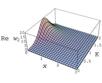
Figure 1: The real part of the bosonic mode ${\rm w}_{2,nonherm}(y)$ for ${\rm x}\in[0,3]$ and the nonhermiticity parameter in the range ${\rm K\in[0,2]}$. The rest of the parameters have the following values: $A=1$, $B=2$, $a=0.5$, $K^{\prime}=2$, and $\alpha_{1,2}=1$ in all the figures of this paper.

Figure 2: The imaginary part of the bosonic mode ${\rm w}_{2,nonherm}(y)$ for the same range of ${\rm x}$ and ${\rm K}$.

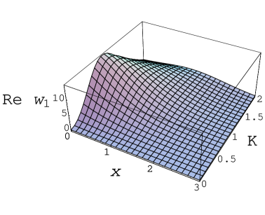
Figure 3: The real part of the fermionic mode ${\rm w}_{1,nonherm}(y)$ for ${\rm x}\in[0,3]$ and the nonhermiticity parameter in the range ${\rm K\in[0,2]}$.

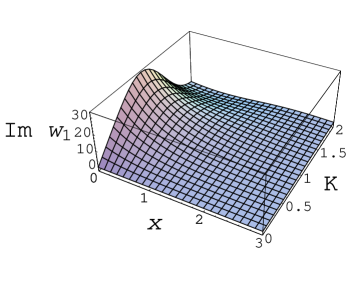
Figure 4: The imaginary part of the fermionic mode ${\rm w}_{1,nonherm}(y)$ for ${\rm x}\in[0,3]$ and ${\rm K\in[0,2]}$.

References

- [1] H.C. Rosu, O. Cornejo-Pérez, R. López-Sandoval, “Classical harmonic oscillator with Dirac-like parameters and possible applications”, J. Phys. A 37, 11699 (2004).
- [2] H.C. Rosu and R. López-Sandoval, “Barotropic FRW cosmologies with a Dirac-like parameter”, Mod. Phys. Lett. A 19, 1529 (2004).
- [3] F. Cooper, A. Khare A, R. Musto, A.Wipf, “Supersymmetry and the Dirac equation”, Ann. Phys. 187, 1 (1988). See also, C.V. Sukumar, “Susy and the Dirac equation for a central Coulomb field”, J. Phys. A 18, L697 (1985); R.J. Hughes, V.A. Kostelecký, M.M. Nieto, “Susy quantum mechanics in a first-order Dirac equation”, Phys. Rev. D 34, 1100 (1986); Y. Nogami and F.M. Toyama, “Supersymmetry aspects of the Dirac equation in one dimension with a Lorentz scalar potential”, Phys. Rev. A 47, 1708 (1993); M. Bellini, R.R. Deza and R. Montemayor, “Mapeo en una mecánica cuántica SUSY para la ecuación de Dirac en D=1+1”, Rev. Mex. Fís. 42, 209 (1996).
- [4] E. Witten, “Dynamical breaking of supersymmetry”, Nucl. Phys. B 188, 513 (1981).
- [5] G. Lévêque et al, “Atomic diffraction from nanostructured optical potentials”, Phys. Rev. A 65, 053615 (2002).