Unambiguous discrimination of special sets of multipartite states using local measurements and classical communication

Abstract

We initially consider a quantum system consisting of two qubits, which can be in one of two nonorthogonal states, $|\Psi_{0}\rangle$ and$|\Psi_{1}\rangle$. We distribute the qubits to two parties, Alice and Bob. They each measure their qubits and then compare their measurement results to determine which state they were sent. This procedure is error-free, which implies that it must sometimes fail. In addition, no quantum memory is required; it is not necessary for one of the qubits to be stored until the result of the measurement on the other is known. We consider the cases in which, should failure occur, both parties receive a failure signal or only one does. In the latter case, if the two states share the same Schmidt basis, the states can be discriminated with the same failure probability that would be obtained if the qubits were measured together. This scheme is sufficiently simple that it can be generalized to multipartite qubit, and qudit, states. Applications to quantum secret sharing are discussed. Finally, we present an optical scheme to experimentally realize the protocol in the case of two qubits.

1 Introduction

Suppose we have two qubits prepared in one of two quantum states, $|\Psi_{0}\rangle$ or $|\Psi_{1}\rangle$. We now give one qubit to Alice and one qubit to Bob. Both parties know that the state is either $|\Psi_{0}\rangle$ or $|\Psi_{1}\rangle$, and their task is to perform local measurements on their qubits and communicate through a classical channel to determine the state they have been given. Alice and Bob can perfectly distinguish between the states using local operations and classical communication only if the states are orthogonal [1]. When $|\Psi_{0}\rangle$ and$|\Psi_{1}\rangle$ are not orthogonal, Alice and Bob can use two different strategies to distinguish between the states.

The first one is the minimum error state discrimination approach. In this case, after Alice and Bob measure their qubits, they have to give a conclusive answer about the state; they are not allowed to give “don’t know” as an answer. However, since the states are not orthogonal, the price that the two parties must pay for giving a definite answer is the chance that they will make a mistake and incorrectly identify the state. The minimum probability of making a wrong guess, when each state is equally likely, is [2]

$$p_{E}=\frac{1}{2}(1-\sqrt{1-|\langle\Psi_{0}|\Psi_{1}\rangle|^{2}})$$ (1)

An alternative approach to the state discrimination problem, is the unambiguous state discrimination method. In this case, some measurement outcomes are allowed to be inconclusive; that is Alice and Bob might fail to identify the state, but if they succeed they will not make an error. If each state is equally likely and both qubits are measured together, then the optimal probability to successfully and unambiguously distinguish the states is [3, 4, 5]

$$p_{idp}=1-|\langle\Psi_{0}|\Psi_{1}\rangle|.$$ (2)

The probability of getting an inconclusive result, which provides no information about the state, is $1-p_{idp}$. This success probability can also be achieved if the qubits are measured separately, one by Alice and one by Bob, and they are allowed to communicate through a classical channel [2, 6]. In this procedure, Alice makes a projective measurement on her qubit that gives her no information about the state, and she then communicates the result of her measurement to Bob. Based on this information, Bob is able to make a measurement on his qubit that allows him to decide, with a success probability of $p_{idp}$, what the initial state was.

If one wants to use this procedure as part of a quantum communication scheme, in particular for secret sharing, there are difficulties. In a secret sharing scheme, Alice and Bob are sent parts of a message or key by a third party, Charlie, and these parts have to be combined in order for the message or key to be revealed [7, 8, 9]. The first problem, then, is that if the parts are to be combined at a time significantly later than when they were sent, quantum memory is required, i.e. the qubits have to be protected against decoherence for a long time. If one attempts to surmount this difficulty by having the parties measure their qubits immediately upon receiving them, one is faced with the problem that the information gain is asymmetric. Alice learns nothing about the key, and Bob learns everything. The only way this could be useful is if Alice and Bob are in the same location and are to use the key immediately. If they are in separate locations and will be using the key later, another procedure is required.

In a previous paper we discussed such a scheme [10]. In it, both parties measure their qubit immediately upon receiving it, each obtaining a result of either $0$ or $1$. There are four sets of results: $\{0,0\}$, $\{1,1\}$,$\{0,1\}$, and $\{1,0\}$. The result $\{0,0\}$ corresponds to $|\Psi_{0}\rangle$, the result $\{1,1\}$ corresponds to $|\Psi_{1}\rangle$, and the results $\{0,1\}$, and $\{1,0\}$ correspond to failure. It was shown that in the case that the two states have the same Schmidt basis, the probability of successfully identifying the state is given by $p_{idp}$. This procedure can be used in a secret-sharing scheme; the set of measurement results obtained by Alice and Bob, which is classical information, can be stored indefinitely and compared at a later time to reveal the key.

This scheme does, however, have a drawback. The key bits for which the measurement failed, and which, therefore, must be discarded, are only identified after Alice and Bob have compared their bit strings. It would be much better if the bits that must be discarded could be identified immediately. The previous procedure requires that Alice and Bob get together and then tell Charlie which bits are good and which are not. He can then send them a message. A procedure in which the failed bits are immediately identified, allows Charlie to send Alice and Bob the two-qubit states from which the key bits can be extracted, discard the failed bits, and then immediately send them the message. At some later time, Alice and Bob can get together, combine their bit strings to get the key, and then read the message, without further input from Charlie. This latter scheme is much more flexible.

This can be accomplished by adding a third measurement result for one or both of the parties. If this added result is obtained, the measurement has failed to distinguish the states. In this paper, we will examine both the case in which both parties have three measurement outcomes, $0$, $1$, or $f$ for failure to distinguish, or only one does. In the latter case, the remaining party has only the outcomes $0$ and $1$. We shall first examine the case in which both Alice and Bob receive a failure indication when the measurement fails. We shall find that this kind of scheme is impossible for two-qubit states if both states are to be detected with a nonzero probability. We shall then show that a procedure in which only one of the parties receives a failure signal is possible, and construct the necessary POVM. In addition, we shall show how this procedure can be implemented optically. The qubits are the polarization states of photons. Two photon states are created and one photon each is sent to Alice and Bob. Using linear optics they can perform the necessary measurements and identify, with a certain probability, which of two possible two-photon states was sent. Finally, we shall show how the procedure in which only one party receives a failure signal can be generalized to $N$ parties, and to qudits rather than qubits. The case of $N$ parties discriminating among three $N$-qutrit states is discussed in detail.

2 Failure indication received by both parties

As discussed in the Introduction, we shall first assume that the measurements that Alice and Bob make have three possible outcomes, $0$, $1$, and $f$, which denotes failure to distinguish . The POVM operators that characterize the measurements are $\{A_{0},A_{1},A_{f}\}$ for Alice and $\{B_{0},B_{1},B_{f}\}$ for Bob. These operators satisfy

$$I_{A}=\sum_{j=0,1,f}A_{j}^{\dagger}A_{j}\hskip 28.45274ptI_{B}=\sum_{j=0,1,f}B_{j}^{\dagger}B_{j},$$ (3)

where $I_{A}$ is the identity on $\mathcal{H}_{A}$, the Hilbert space of Alice’s qubit, and $I_{B}$ is the identity on $\mathcal{H}_{B}$, the space of Bob’s qubit. We suppose that measurement results $\{0,0\}$ (Alice obtains $0$ and Bob also obtains $0$) and $\{1,1\}$ correspond to $|\Psi_{1}\rangle$, and $\{0,1\}$ and $\{1,0\}$ correspond to $|\Psi_{0}\rangle$. The reason for this choice is that we do not want Alice or Bob to be able to tell from only the result of their measurement which state was sent. For example, if Alice always measured $0$ when $|\Psi_{0}\rangle$ was sent and $1$ when $|\Psi_{1}\rangle$ was sent, then she would have no need of any information from Bob to determine the identity of the state. Consequently, for each state, Alice and Bob must have the possibility of receiving either a $0$ or a $1$. The correspondence between states and measurement results is one of only two choices that satisfies this condition (the other simply switches the measurement results corresponding to $|\Psi_{0}\rangle$ and $|\Psi_{1}\rangle$ ). The condition that no errors are allowed requires that

$$A_{0}B_{0}|\Psi_{0}\rangle=0\hskip 28.45274ptA_{1}B_{1}|\Psi_{0}\rangle=0$$ (4)

$$A_{0}B_{1}|\Psi_{1}\rangle=0\hskip 28.45274ptA_{1}B_{0}|\Psi_{1}\rangle=0,$$ (5)

and the condition that, if the measurement fails, then both Alice and Bob find the result $f$, is

$$A_{f}B_{j}|\Psi_{k}\rangle=0\hskip 28.45274ptA_{j}B_{f}|\Psi_{k}\rangle=0,$$ (6)

where $j=0,1$ and $k=0,1$

Expressing $|\Psi_{0}\rangle$ and $|\Psi_{1}\rangle$ in their Schmidt bases we have

$$|\Psi_{0}\rangle=\sum_{l=0}^{1}\sqrt{\lambda_{0l}}|u_{Al}\rangle\otimes|u_{Bl}\rangle$$ (7)

$$|\Psi_{1}\rangle=\sum_{l=0}^{1}\sqrt{\lambda_{1l}}|v_{Al}\rangle\otimes|v_{Bl}\rangle,$$ (8)

where $\{u_{A0},u_{A1}\}$ and $\{v_{A0},v_{A1}\}$ are orthonormal bases for Alice’s space, and $\{u_{B0},u_{B1}\}$ and $\{v_{B0},v_{B1}\}$ are orthonormal bases for Bob’s space. The coefficients $\lambda_{0l}$ and $\lambda_{1l}$ where $l=0,1$, are the eigenvalues of the reduced density matrices corresponding to $|\Psi_{0}\rangle$ and $|\Psi_{1}\rangle$, respectively. Substituting this representation into the conditions in the previous paragraph, we find, first, that the condition $A_{f}B_{j}|\Psi_{0}\rangle=0$ implies that

$$\sqrt{\lambda_{00}}A_{f}|u_{A0}\rangle\otimes B_{j}|u_{B0}\rangle=-\sqrt{\lambda_{01}}A_{f}|u_{A1}\rangle\otimes B_{j}|u_{B1}\rangle.$$ (9)

This is only possible if $A_{f}|u_{A0}\rangle$ is parallel to $A_{f}|u_{A1}\rangle$ and if $B_{j}|u_{B0}\rangle$ is parallel to $B_{j}|u_{B1}\rangle$. Then, we have, for some vectors $|\eta_{Af}\rangle$ and $|\eta_{Bj}\rangle$, that

$$A_{f}|u_{A0}\rangle=c_{0f}|\eta_{Af}\rangle B_{j}|u_{B0}\rangle=d_{j0}|\eta_{Bj}\rangle$$

$$A_{f}|u_{A1}\rangle=c_{1f}|\eta_{Af}\rangle B_{j}|u_{B1}\rangle=d_{j1}|\eta_{Bj}\rangle,$$ (10)

where $c_{lf}$ and $d_{jl}$ are constants, and $\|\eta_{Af}\|=1$ and $\|\eta_{Bj}\|=1$. We can then express $A_{f}$ as

$$A_{f} = |\eta_{Af}\rangle(c_{0f}\langle u_{A0}|+c_{1f}\langle u_{A1}|)$$ (11)

$$= x_{f}|\eta_{Af}\rangle\langle r_{f}|,$$

where

$$|r_{f}\rangle=\frac{1}{(|c_{0f}|^{2}+|c_{1f}|^{2})^{1/2}}(c_{0f}^{\ast}|u_{A0}\rangle+c_{1f}^{\ast}|u_{A1}\rangle).$$ (12)

Similarly, we find that for $j=0,1,f$

$$A_{j}=x_{j}|\eta_{Aj}\rangle\langle r_{j}|\hskip 28.45274ptB_{j}=y_{j}|\eta_{Bj}\rangle\langle s_{j}|,$$ (13)

where $|\eta_{Aj}\rangle$, $|\eta_{Bj}\rangle$, $|r_{j}\rangle$, and $|s_{j}\rangle$ are unit vectors, and the constants $x_{j}$ and $y_{j}$ are yet to be determined.

We can substitute the above expressions for the POVM operators into the conditions for no errors and for simultaneous failure results, Eqs. (4) and (6). The equations containing $|\Psi_{0}\rangle$ are

$$\sqrt{\lambda_{00}}\langle r_{0}|u_{A0}\rangle\langle s_{0}|u_{B0}\rangle+\sqrt{\lambda_{01}}\langle r_{0}|u_{A1}\rangle\langle s_{0}|u_{B1}\rangle=0$$

$$\sqrt{\lambda_{00}}\langle r_{1}|u_{A0}\rangle\langle s_{1}|u_{B0}\rangle+\sqrt{\lambda_{01}}\langle r_{1}|u_{A1}\rangle\langle s_{1}|u_{B1}\rangle=0$$

$$\sqrt{\lambda_{00}}\langle r_{f}|u_{A0}\rangle\langle s_{j}|u_{B0}\rangle+\sqrt{\lambda_{01}}\langle r_{f}|u_{A1}\rangle\langle s_{j}|u_{B1}\rangle=0$$

$$\sqrt{\lambda_{00}}\langle r_{j}|u_{A0}\rangle\langle s_{f}|u_{B0}\rangle+\sqrt{\lambda_{01}}\langle r_{j}|u_{A1}\rangle\langle s_{f}|u_{B1}\rangle=0.$$ (14)

Defining the matrix

$$M^{(0)}=\left(\begin{array}[]{cc}\sqrt{\lambda_{00}}&0\\ 0&\sqrt{\lambda_{01}}\end{array}\right)$$ (15)

and the vectors

$$\overline{r}_{j}^{*}=\left(\begin{array}[]{c}\langle r_{j}|u_{A0}\rangle\\ \langle r_{j}|u_{A1}\rangle\end{array}\right)\hskip 28.45274pt\overline{s}_{j}=\left(\begin{array}[]{c}\langle s_{j}|u_{B0}\rangle\\ \langle s_{j}|u_{B1}\rangle\end{array}\right),$$ (16)

we can express the above equations as

$$\overline{r}_{0}^{*}\cdot M^{(0)}\overline{s}_{0}=0\hskip 28.45274pt \overline{r}_{f}^{*}\cdot M^{(0)}\overline{s}_{j}=0$$

$$\overline{r}_{1}^{*}\cdot M^{(0)}\overline{s}_{1}=0\hskip 28.45274pt \overline{r}_{j}^{*}\cdot M^{(0)}\overline{s}_{f}=0.$$ (17)

It is straightforward to show that if both $\lambda_{00}$ and $\lambda_{01}$ are not zero, and if $\overline{w}^{\ast}\cdot M^{(0)}\overline{x}=0$ and $\overline{w}^{\ast}\cdot M^{(0)}\overline{y}=0$, for $\overline{w}\neq 0$, then $\overline{x}$ is a multiple of $\overline{y}$. Applying this to Eqs. (2), we see that $\overline{s}_{1}$ is a multiple of $\overline{s}_{f}$ and that $\overline{s}_{0}$ is also a multiple of $\overline{s}_{f}$ . The fact that the three vectors, $\overline{s}_{0}$, $\overline{s}_{1}$ and $\overline{s}_{f}$, are parallel violates the condition $I_{B}=\sum_{j=0,1,f}y_{j}|s_{j}\rangle\langle s_{j}|$. If we attempt to circumvent this by choosing either $|r_{0}\rangle$ or $|r_{1}\rangle$ equal to zero, we still find that $\overline{s}_{0}$, $\overline{s}_{1}$ and $\overline{s}_{f}$ are parallel.

The cases in which either $\lambda_{00}$ or $\lambda_{01}$ are zero also need to be examined, but the conclusion is the same; it is not possible to construct a POVM that satisfies Eqs. (4) and (6) and for which both $|\Psi_{0}\rangle$ and $|\Psi_{1}\rangle$ have a nonzero probability of being detected. There are simply too many restrictions on the POVM elements and they cannot all be satisfied. Therefore, we cannot construct a POVM that is error-free, and for which Alice and Bob receive simultaneous failure signals, when the procedure fails. It should be noted, as shown in [10], that if qutrits are used instead of qubits, an error-free POVM with simultaneous failure signals is possible.

3 Failure signal received by one party

In light of what we have just learned it makes sense to now consider the situation in which only one party receives a failure indication when the measurement fails. In particular, both parties will have the possibility of receiving a failure signal, and if either one of them does (even if the other does not), then the procedure has failed. No assumption is made about which party will receive a failure signal. We shall also consider a special case, that in which $|\Psi_{0}\rangle$ and $|\Psi_{1}\rangle$ have the same Schmidt bases and are given by

$$|\Psi_{0}\rangle=\cos\theta_{0}|00\rangle+\sin\theta_{0}|11\rangle$$

$$|\Psi_{1}\rangle=\cos\theta_{1}|00\rangle+\sin\theta_{1}|11\rangle.$$ (18)

The conditions that no errors are allowed are the same as before

$$A_{0}B_{0}|\Psi_{0}\rangle=0\hskip 28.45274ptA_{1}B_{1}|\Psi_{0}\rangle=0$$

$$A_{0}B_{1}|\Psi_{1}\rangle=0\hskip 28.45274ptA_{1}B_{0}|\Psi_{1}\rangle=0.$$ (19)

These conditions imply, as before, that for $j=0,1$

$$A_{j}=x_{j}|\eta_{Aj}\rangle\langle r_{j}|\hskip 28.45274ptB_{j}=y_{j}|\eta_{Bj}\rangle\langle s_{j}|,$$

and we shall express the vectors $|r_{j}\rangle$ and $|s_{j}\rangle$ in the basis $\{|0\rangle,|1\rangle\}$ as

$$|r_{0}\rangle=a_{0}|0\rangle+a_{1}|1\rangle\hskip 28.45274pt|s_{0}\rangle=c_{0}|0\rangle+c_{1}|1\rangle$$

$$|r_{1}\rangle=b_{0}|0\rangle+b_{1}|1\rangle\hskip 28.45274pt|s_{1}\rangle=d_{0}|0\rangle+d_{1}|1\rangle$$ (21)

The no-error conditions can now be expressed as

$$(\langle r_{0}|\langle s_{0}|)|\Psi_{0}\rangle=0\hskip 28.45274pt(\langle r_{1}|\langle s_{1}|)|\Psi_{0}\rangle=0$$

$$(\langle r_{0}|\langle s_{1}|)|\Psi_{1}\rangle=0\hskip 28.45274pt(\langle r_{1}|\langle s_{0}|)|\Psi_{1}\rangle=0.$$ (22)

Defining the ratios

$$z_{0}=\frac{a_{1}}{a_{0}} z_{1}=\frac{b_{1}}{b_{0}}$$ (23)

$$z_{2}=\frac{c_{1}}{c_{0}} z_{3}=\frac{d_{1}}{d_{0}},$$ (24)

Equations (3) become

$$1+z_{0}^{\ast}z_{2}^{\ast}\tan\theta_{0}=0\hskip 28.45274pt1+z_{1}^{\ast}z_{3}^{\ast}\tan\theta_{0}=0$$

$$1+z_{0}^{\ast}z_{3}^{\ast}\tan\theta_{1}=0\hskip 28.45274pt1+z_{1}^{\ast}z_{2}^{\ast}\tan\theta_{1}=0$$ (25)

A necessary condition for these equations to have a solution is that $\tan\theta_{0}=\pm\tan\theta_{1}$. We are not interested in the case where $\tan\theta_{0}=\tan\theta_{1}$, since this implies that our states are identical. We wish to examine the case where $\tan\theta_{0}=-\tan\theta_{1}$, which implies that $\theta_{1}=-\theta_{0}$. Hence, our two states can be expressed as

$$|\Psi_{0}\rangle=\cos\theta_{0}|00\rangle+\sin\theta_{0}|11\rangle$$

$$|\Psi_{1}\rangle=\cos\theta_{0}|00\rangle-\sin\theta_{0}|11\rangle$$ (26)

In this case, we find

$$z_{2}=-\frac{1}{z_{0}}\cot\theta_{0}\hskip 28.45274ptz_{3}=\frac{1}{z_{0}}\cot\theta_{0}\hskip 28.45274ptz_{1}=-z_{0}.$$ (27)

We can now express the vectors $|r_{j}\rangle$ and $|s_{j}\rangle$ as

$$|r_{0}\rangle=\frac{1}{\sqrt{1+|z_{0}|^{2}}}(|0\rangle+z_{0}|1\rangle)$$

$$|r_{1}\rangle=\frac{1}{\sqrt{1+|z_{0}|^{2}}}(|0\rangle-z_{0}|1\rangle)$$

$$|s_{0}\rangle=\sqrt{\frac{|z_{0}|^{2}}{|z_{0}|^{2}+{\cot\theta_{0}}^{2}}}(|0\rangle-\frac{\cot\theta_{0}}{z_{0}}|1\rangle)$$

$$|s_{1}\rangle=\sqrt{\frac{|z_{0}|^{2}}{|z_{0}|^{2}+{\cot\theta_{0}}^{2}}}(|0\rangle+\frac{\cot\theta_{0}}{z_{0}}|1\rangle).$$

The parameter $z_{0}$ is yet to be determined.

The failure operators for Alice and Bob can be expressed as

$$A_{f}^{\dagger}A_{f}=I_{A}-|x_{0}|^{2}|r_{0}\rangle\langle r_{0}|-|x_{1}|^{2}|r_{1}\rangle\langle r_{1}|$$ (28)

$$B_{f}^{\dagger}B_{f}=I_{B}-|y_{0}|^{2}|s_{0}\rangle\langle s_{0}|-|y_{1}|^{2}|s_{1}\rangle\langle s_{1}|,$$ (29)

where $x_{j}$, $y_{j}$, and $z_{0}$, where $j=0,1$, must be chosen so that these are positive operators. The condition $A_{f}^{\dagger}A_{f}\geq 0$ implies that

$$I_{A}-\frac{|x_{0}|^{2}}{1+|z_{0}|^{2}}(|0\rangle+z_{0}|1\rangle)(\langle 0|+z_{0}^{\ast}\langle 1|)-\frac{|x_{1}|^{2}}{1+|z_{0}|^{2}}(|0\rangle-z_{0}|1\rangle)(\langle 0|-z_{0}^{\ast}\langle 1|)\geq 0,$$ (30)

or, in matrix form

$$M_{A}=\left(\begin{array}[]{cc}1-\frac{|x_{0}|^{2}+|x_{1}|^{2}}{1+|z_{0}|^{2}}&-\frac{z_{0}^{\ast}(|x_{0}|^{2}-|x_{1}|^{2})}{1+|z_{0}|^{2}}\\ -\frac{z_{0}(|x_{0}|^{2}-|x_{1}|^{2})}{1+|z_{0}|^{2}}&1-\frac{|z_{0}|^{2}(|x_{0}|^{2}+|x_{1}|^{2})}{1+|z_{0}|^{2}}\end{array}\right)\geq 0.$$ (31)

This matrix will be postive if both ${\rm Tr}M_{A}\geq 0$, which implies that

$$2-(|x_{0}|^{2}-|x_{1}|^{2})\geq 0,$$ (32)

and $\det M_{A}\geq 0$, which implies

$$(1+|z_{0}|^{2})^{2}(1-(|x_{0}|^{2}+|x_{1}|^{2}))+4|z_{0}|^{2}|x_{0}|^{2}|x_{1}|^{2}\geq 0.$$ (33)

Similar conditions are found from the requirement that $B_{f}^{\dagger}B_{f}\geq 0$.

Our goal is to minimize the total failure probability, $p_{f}$, which is found by summing over all measurement results that contain a failure signal, and is

$$p_{f}=\frac{1}{2}\sum_{k=0}^{1}\langle\Psi_{k}|(A_{f}^{\dagger}A_{f}\otimes I_{B}+I_{A}\otimes B_{f}^{\dagger}B_{f}-A_{f}^{\dagger}A_{f}\otimes B_{f}^{\dagger}B_{f})|\Psi_{k}\rangle.$$ (34)

We have assumed that the probability of receiving either $|\Psi_{0}\rangle$ or $|\Psi_{1}\rangle$ is the same, i.e. $1/2$. We shall specialize to the case $x_{0}=x_{1}$ and $y_{0}=y_{1}$. As we shall see, this will still allow us to obtain the minimum achievable failure probability. Doing so we find that

$$A_{f}^{\dagger}A_{f} = I_{A}-\frac{2|x_{0}|^{2}}{1+|z_{0}|^{2}}(|0\rangle\langle 0|+|z_{0}|^{2}|1\rangle\langle 1|)$$

$$B_{f}^{\dagger}B_{f} = I_{B}-\frac{2|y_{0}|^{2}|z_{0}|^{2}}{|z_{0}|^{2}+\cot^{2}\theta_{0}}\left(|0\rangle\langle 0|+\frac{\cot^{2}\theta_{0}}{|z_{0}|^{2}}|1\rangle\langle 1|\right).$$ (35)

It is clear from Eq. (34) that the failure probability will be a minimum when $|x_{0}|$ and $|y_{0}|$ are as large as possible, subject to the constraint that the operators $A_{f}^{\dagger}A_{f}$ and $B_{f}^{\dagger}B_{f}$ are positive. From the above equations, we see that this implies that if $|z_{0}|\leq 1$, then $|x_{0}|^{2}=(1+|z_{0}|^{2})/2$ and

$$A_{f}^{\dagger}A_{f}=(1-|z_{0}|^{2})|1\rangle\langle 1|,$$ (36)

and if $|z_{0}|\geq 1$, then $|x_{0}|^{2}=[1+(1/|z_{0}|^{2})]/2$, and

$$A_{f}^{\dagger}A_{f}=\left(1-\frac{1}{|z_{0}|^{2}}\right)|0\rangle\langle 0|.$$ (37)

We also have that if $\cot^{2}\theta_{0}\leq|z_{0}|^{2}$, then $|y_{0}|^{2}=[1+(\cot\theta_{0}/|z_{0}|)^{2}]/2$ and

$$B_{f}^{\dagger}B_{f}=\left(1-\frac{\cot^{2}\theta_{0}}{|z_{0}|^{2}}\right)|1\rangle\langle 1|,$$ (38)

and if $\cot^{2}\theta_{0}\geq|z_{0}|^{2}$, then $|y_{0}|^{2}=[1+(|z_{0}|/\cot\theta_{0})^{2}]/2$ and

$$B_{f}^{\dagger}B_{f}=\left(1-\frac{|z_{0}|^{2}}{\cot^{2}\theta_{0}}\right)|0\rangle\langle 0|.$$ (39)

Let us consider the case when $|z_{0}|\leq 1$ and $0\leq\theta\leq\pi/4$, which implies that Eqs. (36) and (39) apply. We then have that the failure probability is given by

$$p_{f}=1-2|z_{0}|^{2}\sin^{2}\theta_{0},$$ (40)

and it is clear that this is minimized by choosing $|z_{0}|=1$. This gives us

$$p_{f}=\cos(2\theta_{0}),$$ (41)

which is equal to the optimal failure probability for distinguishing the states $|\Psi_{0}\rangle$ and $|\Psi_{1}\rangle$. This failure probability is given by

$$1-p_{idp}=|\langle\Psi_{1}|\Psi_{0}\rangle|=\cos(2\theta_{0}).$$ (42)

This implies that by using this procedure, we can distinguish the states just as well by measuring the qubits separately and comparing the results as we can by performing a joint measurement on both of them.

Let us now summarize the results of the preceding calculations. The states we are distinguishing are given in Eq. (3), with $0\leq\theta\leq\pi/4$. Alice’s POVM elements are $|r_{j}\rangle\langle r_{j}|$, for $j=0,1$, with

$$|r_{0}\rangle = \frac{1}{\sqrt{2}}(|0\rangle+|1\rangle)$$

$$|r_{1}\rangle = \frac{1}{\sqrt{2}}(|0\rangle-|1\rangle),$$ (43)

and $A_{f}=0$. This implies that Alice will only obtain the results $0$ or $1$ for her measurement, she will never receive a failure result. In fact, she simply performs a projective measurement. Bob’s POVM elements are

$$B_{j}^{\dagger}B_{j}=\frac{1}{2}(1+\tan^{2}\theta_{0})|s_{j}\rangle\langle s_{j}|$$ (44)

for $j=0,1$, with

$$|s_{0}\rangle = \sin\theta_{0}|0\rangle-\cos\theta_{0}|1\rangle$$

$$|s_{1}\rangle = \sin\theta_{0}|0\rangle+\cos\theta_{0}|1\rangle,$$ (45)

and, corresponding to the failure result,

$$B_{f}^{\dagger}B_{f}=(1-\tan^{2}\theta_{0})|0\rangle\langle 0|$$ (46)

.

Examining these results, we can now see, in a simple way, how this procedure works. Define the single qubit states $|\psi_{j}\rangle$, for $j=0,1$ as

$$|\psi_{j}\rangle=\cos\theta_{0}|0\rangle+(-1)^{j}\sin\theta_{0}|1\rangle.$$ (47)

When Alice performs her measurement, she obtains either $0$ or $1$. If she obtains $0$, then Bob is left with the state $|\psi_{0}\rangle$ if $|\Psi_{0}\rangle$ was sent, and $|\psi_{1}\rangle$ if $|\Psi_{1}\rangle$ was sent. If she obtains $1$, then Bob is left with the state $|\psi_{1}\rangle$ if $|\Psi_{0}\rangle$ was sent, and $|\psi_{0}\rangle$ if $|\Psi_{1}\rangle$ was sent. In either case, Bob is faced with discriminating between the non-orthogonal states $|\psi_{0}\rangle$ and $|\psi_{1}\rangle$. He then applies the optimal POVM to distinguish between these states, and if he succeeds, he knows which of the two states he has. What he does not know, is which of his single-qubit states corresponds to $|\Psi_{0}\rangle$, and which to $|\Psi_{1}\rangle$. It is this bit of information that the result of Alice’s measurement contains. Only by combining the results of their measurements can Alice and Bob deduce which state was sent.

The analysis in the preceding paragraph immediately allows us to see that there is another solution to the problem of finding a POVM in which one of the parties can receive a failure signal, and that is the one in which the roles of Alice and Bob are interchanged. In that case, Bob makes a projective measurement, and Alice makes a measurement whose results are described by a three-outcome POVM.

It was noted by Virmani, et al. [2], that for any two two-qubit states with the same Schmidt basis, which they called Schmidt correlated, it is possible for Alice to transfer all of the information about the state to Bob by making a measurement in the basis $\{|r_{0}\rangle,|r_{1}\rangle\}$ and telling Bob the result of her measurement. In general Bob’s measurement will depend on the results of Alice’s. What we have seen in this section is that for special choices of the two states, Alice and Bob always make the same measurement, which means they can make the measurement as soon as they receive the particles. They, each, then, posses a classical bit, and by comparing these bits they can tell which state they were sent.

4 Optical realization

We now want to show how this measurement can be realized optically. The states $|\Psi_{0}\rangle$ and $|\Psi_{1}\rangle$ are two-photon states with the information encoded in the polarization of the photons. We suppose that $|0\rangle$ corresponds to horizontal polarization and $|1\rangle$ to vertical. Alice’s measurement is then straightforward; she sends her photon through a polarization beam splitter. A horizontally polarized photon incident on this device will continue in a straight line while a vertically polarized photon will be deflected by ninety degrees. Alice orients her polarization beam splitter so that a photon in the polarization state $(|0\rangle+|1\rangle)/\sqrt{2}$ is transmitted and one in the state $(|0\rangle-|1\rangle)/\sqrt{2}$ is deflected. She has detectors in both paths, and she simply observes which one clicks.

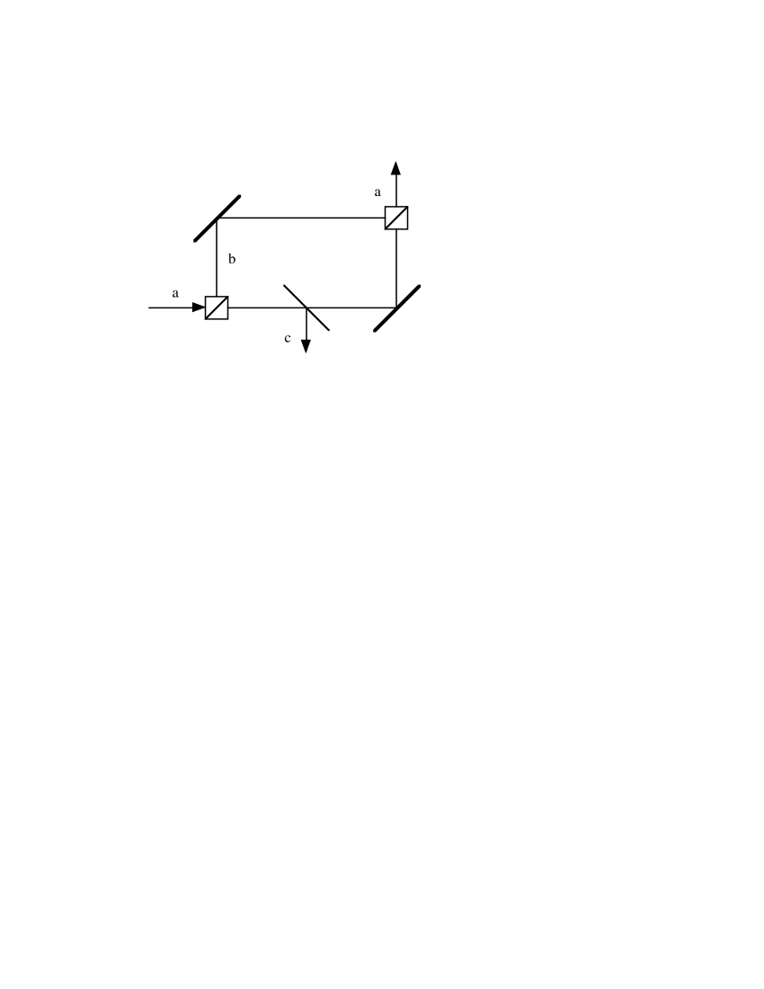
Figure 1: Interferometer for realizing three-outcome POVM. The photon enters in mode $a$ and encounters a polarization beam splitter. Its vertically polarized part is refelected into mode $b$, while its horizontally polarized part is transmitted in mode $a$. In its passage through the device, the photon encounters a polarization insensitive beam splitter and one more polarization beam spliter. If the photon emerges in mode $c$, the measurement has failed, and if it emerges in mode $a$, it has succeeded.

Bob’s measurement is more complicated, but it has been worked out by Huttner, et al. [11]. They presented two implementations of the POVM, one in which the failure signal can be detected explicitly and one in which it cannot, and demonstrated the second experimentally. We shall describe their first scheme. It makes use of two polarization beam splitters, and one standard, polarization-insensitive beam splitter, and is depicted in Fig. 1. The input state, which is either $|\psi_{0}\rangle$ or $|\psi_{1}\rangle$, is sent into the first polarization beam splitter in mode $a$. The vertically polarized part of the state is deflected into mode $b$, while the horizontally polarized part continues in mode $a$. If the input state is given by $|\phi_{in}\rangle_{a}=\alpha|0\rangle_{a}+\beta|1\rangle_{a}$, where the subscripts on the states denote the mode, we have that just after the first polarization beam splitter

$$|\phi_{in}\rangle_{A}\rightarrow\alpha|0\rangle_{a}+\beta|1\rangle_{b}.$$ (48)

The beam splitter transmits a photon with transmissivity $t$ and reflects it with reflectivity $r$. This implies that after passing through the beam splitter the state $|0\rangle_{a}$ becomes $t|0\rangle_{a}+r|0\rangle_{c}$. Finally, after the second polarization beam splitter, the output state, $|\phi_{out}\rangle$ is

$$|\phi_{out}\rangle=\alpha t|0\rangle_{a}+\beta|1\rangle_{a}+\alpha r|0\rangle_{c}.$$ (49)

Choosing $t=\tan\theta_{0}$, we have that if the input state is $|\psi_{0}\rangle$, then

$$|\phi_{out}\rangle=\sin\theta_{0}(|0\rangle_{a}+|1\rangle_{a})+\sqrt{\cos 2\theta_{0}}|0\rangle_{c},$$ (50)

and if the input state is $|\psi_{1}\rangle$, then

$$|\phi_{out}\rangle=\sin\theta_{0}(|0\rangle_{a}-|1\rangle_{a})+\sqrt{\cos 2\theta_{0}}|0\rangle_{c}.$$ (51)

Note that the parts of the two output states in the $a$ mode have orthogonal polarizations, and can be distinguished by orienting a third polarzation beam splitter so that $(|0\rangle_{a}+|1\rangle_{a})/\sqrt{2}$ is transmitted and $(|0\rangle_{a}-|1\rangle_{a})/\sqrt{2}$ is deflected. If the photon is detected in mode $c$, the procedure has failed. Note that both Alice’s and Bob’s measurements can be realized using only linear optics.

5 More than two parties

It is relatively easy to generalize the procedure in section 3 to divide the information about which of two states was sent among any number of parties. We shall show how to do this for both qubits and for qutrits.

Let us start with two $N$-qubit states

$$|\Psi_{0}\rangle = \cos\theta_{0}|00\ldots 0\rangle+\sin\theta_{0}|11\dots 1\rangle$$

$$|\Psi_{1}\rangle = \cos\theta_{0}|00\ldots 0\rangle-\sin\theta_{0}|11\dots 1\rangle,$$ (52)

where $0\leq\theta_{0}\leq\pi/4$. Each of the qubits is sent to one of $N$ parties, $A_{1},\ldots A_{N}$. Each of the parties, $A_{1}$ through $A_{N-1}$ measures their qubit in the $\{r_{0},r_{1}\}$ basis (see Eq. (3)), and $A_{N}$ performs the unambiguous-state discrimination procedure for the states $|\psi_{0}\rangle$ and $|\psi_{1}\rangle$ (see Eq. (47)). If parties $A_{1}$ through $A_{N-1}$ obtained $n_{0}$ results of $|r_{0}\rangle$ and $n_{1}$ results of $|r_{1}\rangle$, then the states that $A_{N}$ is distinguishing between are

$$|\psi_{0N}\rangle = \cos\theta_{0}|0\rangle+(-1)^{n_{1}}\sin\theta_{0}|1\rangle$$

$$|\psi_{1N}\rangle = \cos\theta_{0}|0\rangle-(-1)^{n_{1}}\sin\theta_{0}|1\rangle,$$ (53)

i.e. $A_{N}$’s qubit will be in the state $|\psi_{0N}\rangle$ if the state $|\Psi_{0}\rangle$ was sent and $|\psi_{1N}\rangle$ if the state $|\Psi_{1}\rangle$ was sent. In order to ascertain which of the two $N$-qubit states was sent, all of the parties will have to combine their information. If the measurement made by $A_{N}$ succeeds, then she will have obtained either $|\psi_{0}\rangle$ or $|\psi_{1}\rangle$, but she will not, without knowing the measurement results of all of the other parties, know which of these results corresponds to $|\Psi_{0}\rangle$ and which corresponds to $|\Psi_{1}\rangle$.

The procedure can be generalized to particles with more than two internal states, and to demonstrate this we shall consider the case of qutrits. Consider the three $N$-qutrit states

$$|\Psi_{0}\rangle = c_{0}|0\ldots 0\rangle+c_{1}|1\ldots 1\rangle+c_{2}|2\dots 2\rangle$$

$$|\Psi_{1}\rangle = c_{0}|0\ldots 0\rangle+c_{1}\omega|1\ldots 1\rangle+c_{2}\omega^{\ast}|2\dots 2\rangle$$

$$|\Psi_{2}\rangle = c_{0}|0\dots 0\rangle+c_{1}\omega^{\ast}|1\ldots 1\rangle+c_{2}\omega|2\ldots 2\rangle,$$ (54)

where $\omega=\exp(2\pi i/3)$. Define the single qutrit orthonormal basis

$$|\eta_{0}\rangle = \frac{1}{\sqrt{3}}(|0\rangle+|1\rangle+|2\rangle)$$

$$|\eta_{1}\rangle = \frac{1}{\sqrt{3}}(|0\rangle+\omega|1\rangle+\omega^{\ast}|2\rangle)$$

$$|\eta_{2}\rangle = \frac{1}{\sqrt{3}}(|0\rangle+\omega^{\ast}|1\rangle+\omega|2\rangle).$$ (55)

Each of the $N$ qutrits is sent to one of the parties $A_{1}$, …$A_{N}$. Now, parties $A_{1}$ through $A_{N-1}$ perform projective measurements in the basis $\{|\eta_{0}\rangle,|\eta_{1}\rangle,|\eta_{2}\rangle\}$, and suppose that $m_{j}$ of them find their qutrit in the state $|\eta_{j}\rangle$, $j=0,1,2$. The party $A_{N}$ performs the optimal POVM to unambiguously distinguish the states [12, 13]

$$|\psi_{0}\rangle = c_{0}|0\rangle+c_{1}|1\rangle+c_{2}|2\rangle$$

$$|\psi_{1}\rangle = c_{0}|0\rangle+c_{1}\omega|1\rangle+c_{2}\omega^{\ast}|2\rangle$$

$$|\psi_{2}\rangle = c_{0}|0\rangle+c_{1}\omega^{\ast}|1\rangle+c_{2}\omega|2\rangle.$$ (56)

After the parties $A_{1}$ through $A_{N-1}$ have performed their measurements, the qutrit belonging to $A_{N}$ is in one of the three states

$$|\psi_{0N}\rangle = c_{0}|0\rangle+c_{1}\omega^{(m_{2}-m_{1})}|1\rangle+c_{2}\omega^{-(m_{2}-m_{1})}|2\rangle$$

$$|\psi_{1N}\rangle = c_{0}|0\rangle+c_{1}\omega^{(m_{2}-m_{1}+1)}|1\rangle+c_{2}\omega^{-(m_{2}-m_{1}+1)}|2\rangle$$

$$|\psi_{2N}\rangle = c_{0}|0\rangle+c_{1}\omega^{(m_{2}-m_{1}-1)}|1\rangle+c_{2}\omega^{-(m_{2}-m_{1}-1)}|2\rangle.$$ (57)

The qutrit is in the state $\psi_{jN}$ if the original $N$-qutrit state was $\Psi_{j}$, for $j=0,1,2$.

If the measurement made by $A_{N}$ succeeds, she will have found her qutrit in one of the states $\psi_{j}$, $j=0,1,2$. She will not know to which of the original $N$-qutrit states it corresponds, however, without knowing the measurement results of all of the other parties. In particular, we have the correspondence

$$\Psi_{j}\leftrightarrow\psi_{[j+m_{2}-m_{1}\ {\rm mod}3]}.$$ (58)

Therfore, all of the parties must combine their information in order to determine which of the three $N$-qutrit states was originally sent.

Note that in both the case of $N$ qubits and $N$ qutrits, only one party will receive a failure signal if the measurement fails. In addition, the probability of failure is the best possible, i.e. it is the same as it would be if all of the qubits or qutrits were measured together. Consequently, we have not lost anything by measuring the particles separately.

6 Conclusion

We have shown that it is possible to distinguish two non-orthogonal two-qubit states by local measurements and classical communication, making no errors and with one of the parties receiving a failure signal if the procedure fails. Both of the parties make fixed measurements, it is not the case that the measurement made by one party depends on the result obtained by the other. If the procedure succeeds, each party obtains either a $0$ or a $1$, and gains no information about the state from their individual results. However, on combining their results, the parties can identify the state.

This procedure should be useful as a basis for quantum secret sharing. It provides security in the same way as does the B92 protocol for quantum key distribution [14]. An eavesdropper, Eve, who intercepts the two-qubit state cannot indentify it with certainty. The best she can do is to apply the two-state unambiguous state discrimination procedure, which will sometimes fail. When it does, she does not know which state to send on to Alice and Bob, and will, consequently, introduce errors, e.g. Alice and Bob will have detected $|\Psi_{0}\rangle$ when $|\Psi_{1}\rangle$ was sent. These errors can be detected if Alice and Bob publicly compare a subset of their measurements with information provided by the person who sent the states.

There is also some protection against cheating. If Alice cheats by obtaining both qubits, then the best she can do is to apply two-state unambiguous state discrimination to them. Her measurement will sometimes fail, and then she has a problem. She must send a qubit to Bob, but there is no state for this qubit that will make Bob’s measurement fail with certainty. That means that Bob will sometimes obtain incorrect results, i.e. when he and Alice combine their results, they will find that the state they detected was not the one that was sent. Therefore, cheating by Alice will introduce errors.

If Bob has obtained both particles, then he also can apply two-state unambiguous state discrimination to the two-qubit state. If his measurement succeeds, he can just send a qubit in the appropriate state to Alice, and if it fails, he can simply state that it failed. That means that cheating by Bob cannot be detected. However, a modification of the protocol will solve this problem. When the two-qubit state is sent, the person sending the state can announce over a public channel, which of the parties is to make the projective measurement and which is to make the three-outcome POVM. This means that part of the time, Bob will be assigned to make the projective measurement, and then his cheating will be detected. He can, however, not cheat if he is assigned to make the projective measurement, and in that case he will gain partial information about the key and not be detected. One way to address this problem is to combine several received bits into a block, the parity of which is a single key bit. In order for Bob to ascertain the key bit, he would have to know all of the received bits in the block, but the probability that he would can be made very low by choosing the block size sufficiently large.

Secret sharing, then, provides one application of the state discrimination procedures discussed in this paper. Whether there are others is a subject for future work.

References

• [1] J. Walgate, A. Short, L. Hardy, and V. Vedral, Phys. Rev. Lett. 85, 4972 (2000).
• [2] S. Virmani, M. F. Sacchi, M. B. Plenio, and D. Markham, Phys. Lett. A 288, 62 (2001).
• [3] I. D. Ivanovic, Phys. Lett. A 123, 257 (1987).
• [4] D. Dieks, Phys. Lett. A 126, 303 (1988).
• [5] A. Peres, Phys. Lett. A 128, 19 (1988).
• [6] Yi-Xin Chen and Dong Yang, Phys. Rev. A 65, 022320 (2002).
• [7] M. Hillery, V. Bužek, and A. Berthiaume, Phys. Rev. A 59, 1829 (1999).
• [8] A. Karlsson, M. Koashi, and N. Imoto, Phys. Rev. A 59, 162 (1999).
• [9] R. Cleve, D. Gottesman, and H. -K. Lo, Phys. Rev. Lett. 83, 648 (1999).
• [10] M. Hillery and J. Mimih, Phys. Rev. A 67, 042304 (2003).
• [11] B. Huttner, A. Muller, J. D. Gautier, H. Zbinden, and N. Gisin, Phys. Rev. A 54, 3783 (1996).
• [12] A. Peres and D. Terno, J. Phys. A 31, 7105 (1998).
• [13] Y. Sun, M. Hillery, and J. A. Bergou, Phys. Rev. A 64, 022311 (2001).
• [14] C. H. Bennett, Phys. Rev. Lett. 68, 3121 (1992).