Quantifying decoherence in continuous variable systems

Abstract

We present a detailed report on the decoherence of quantum states of continuous variable systems under the action of a quantum optical master equation resulting from the interaction with general Gaussian uncorrelated environments. The rate of decoherence is quantified by relating it to the decay rates of various, complementary measures of the quantum nature of a state, such as the purity, some nonclassicality indicators in phase space and, for two-mode states, entanglement measures and total correlations between the modes. Different sets of physically relevant initial configurations are considered, including one- and two-mode Gaussian states, number states, and coherent superpositions. Our analysis shows that, generally, the use of initially squeezed configurations does not help to preserve the coherence of Gaussian states, whereas it can be effective in protecting coherent superpositions of both number states and Gaussian wave packets.

1 Introduction

Beyond their fundamental interest in the physics of elementary particles (quantum electrodynamics and its standard-model generalizations), in quantum optics, and in condensed matter theory, continuous variable systems are beginning to play an outstanding role in quantum communication and information theory [1, 2], as shown by the first spectacular implementations of deterministic teleportation schemes and quantum key distribution protocols in quantum optical settings [3, 4].

In all such practical instances the information contained in a given quantum state of the system, so precious for the realization of any specific task, is constantly threatened by the unavoidable interaction with the environment. Such an interaction entangles the system of interest with the environment, causing any amount of information to be scattered and lost in the (infinite) Hilbert space of the environment. It is important to remark that this information is irreversibly lost, since the degrees of freedom of the environment are out of the experimental control. The overall process, corresponding to a non unitary evolution of the system, is commonly referred to as decoherence [5, 6]. It is thus of crucial importance to develop proper methods to quantify the rate of decoherence, both for its understanding and for building optimal strategies to reduce and/or suppress it.

In this work we study the decoherence of generic states of continuous variable systems whose evolution is ruled by optical master equations in general Gaussian uncorrelated environments. The rate of decoherence is quantified by analysing the evolution of global entropic measures, of nonclassical indicators and, for two-mode states, of entanglement and correlations quantified by the mutual information and by the logarithmic negativity. Several initial states of major interest are considered.

The plan of the paper is as follows. In Section 2 we introduce the notation and define the systems of interest, together with the quantities we will adopt to quantify decoherence. In Section 3 we introduce and solve the quantum optical master equation and its corresponding phase space diffusive equations, discussing some general properties of the nonunitary evolution. In Sections 4-7 we provide a detailed study of the decoherence of single mode Gaussian states, cat-like states, number states and two-mode Gaussian states. Finally, in Section 8 we review and comment the relevant results.

2 Notation and basic concepts

The system we address is a canonical infinite dimensional system constituted by a set of $n$ ‘modes’. Each mode $i$ is described by a pair of canonical conjugate operators $\hat{x}_{i}$, $\hat{p}_{i}$ acting on a denumerable Hilbert space ${\cal H}_{i}$. The space ${\cal H}_{i}$ is spanned by a number basis $\{|n\rangle_{k}\}$ of eigenstates of the operator $\hat{n}_{k}\equiv a_{k}^{{\dagger}}a_{k}$, which represents the Hamiltonian of the non interacting mode. In terms of the ladder operators $a_{k}$ and $a_{k}^{{\dagger}}$ one has $\hat{x}_{k}=(a_{k}+a_{k}^{{\dagger}})/\sqrt{2}$ and $\hat{p}_{k}=i(a_{k}^{{\dagger}}-a_{k})/\sqrt{2}$. Let us group together the canonical operators in the vector of operators $\hat{R}=(\hat{x}_{1},\hat{p}_{1},\ldots,\hat{x}_{n},\hat{p}_{n})$. The canonical commutation relations regulate the commutation properties of the operators:

$$[\hat{R}_{k},\hat{R}_{l}]=i\Omega_{kl}\;,$$

where $\Omega$ is the symplectic form

$$\Omega=\bigoplus_{i=1}^{n}\omega\,,\quad\omega=\left(\begin{array}[]{cc}0&1\\ -1&0\end{array}\right)\,.$$ (1)

The canonical operators $\hat{R}_{i}$ may be second quantized bosonic field operators or position and momentum operators of a material harmonic oscillator. The eigenstates of $a_{i}$ constitutes the important set of coherent states, which is overcomplete in the Hilbert space ${\cal H}_{i}$. Coherent states result from applying to the vacuum $|0\rangle$ the single-mode Weyl displacement operators $D_{i}(\alpha)=\,{\rm e}^{i\alpha a_{i}^{{\dagger}}-\alpha^{*}a_{i}}$: $|\alpha\rangle_{i}=D_{i}(\alpha)|0\rangle$.

The states of the system are the set of positive trace class operators $\{\varrho\}$ on the Hilbert space ${\cal H}=\otimes_{i=1}^{n}{\cal H}_{i}$. However, the complete description of any quantum state $\varrho$ of such an infinite dimensional system can be provided by one of its $s$-ordered characteristic functions [7]

$$\chi_{s}(X)=\,{\rm Tr}\,[\varrho D_{X}]\,{\rm e}^{s\|X\|^{2}/2}\;,$$ (2)

with $X\in\mathbbm{R}^{2n}$, $\|\centerdot\|$ standing for the Euclidean norm $\mathbbm{R}^{2n}$ and the $n$-mode Weyl operator defined as

$$D_{X}=\,{\rm e}^{i\hat{R}^{T}\Omega X},\quad X\in\mathbbm{R}^{2n}\,.$$

The family of characteristic functions is in turn related, via complex Fourier transform, to the quasi-probability distributions $W_{s}$, which constitutes another set of complete descriptions of the quantum states

$$W_{s}(X)=\frac{1}{\pi^{2}}\int_{{\mathbbm{R}}^{2n}}\,{\rm d}^{2n}K\chi_{s}(K)\,{\rm e}^{iK^{T}\Omega X}\,.$$ (3)

The vector $X$ belongs to the space $\Gamma=({\mathbbm{R}}^{2n},\Omega)$, which is called phase space in analogy with classical Hamiltonian dynamics. As well known, there exist states for which the function $W_{s}$ is not a regular probability distribution for any $s$, because it can in general be singular or assume negative values. Note that the value $s=-1$ corresponds to the Husimi ‘Q-function’ $W_{-1}(X)=\langle X|\varrho|X\rangle/\pi$, $|X\rangle$ being a tensor product of coherent states satisfying

$$a_{i}|X\rangle=\frac{X_{2i-1}+iX_{2i}}{\sqrt{2}}|X\rangle\quad\forall i=1,\ldots n\,,$$ (4)

and always yields a regular probability distribution. The case $s=0$ correponds to the so called Wigner function, which will be denoted simply by $W$. Likewise, for the sake of simplicity, $\chi$ will stand for the simmetrically ordered characteristic function $\chi_{0}$.

As a meausure of ‘nonclassicality’ of the quantum state $\varrho$, the quantity $\tau_{\varrho}$, referred to as ‘nonclassical depth’, has been proposed in Ref. [8] and subsequently employed by many authors

$$\tau_{\varrho}=\frac{1-\bar{s}_{\varrho}}{2}\;,$$ (5)

where $\bar{s}_{\varrho}$ is the supremum of the set of values $\{s\}$ for which the quasiprobability function $W_{s}$ associated to the state $\varrho$ can be regarded as a (positive semidefinite and non singular) probability distribution. We mention that a nonzero nonclassical depth has been shown to be a prerequisite for the generation of continuous variable entanglement [9] and is strictly related to the efficiency of teleportation protocols [10]. As one should expect, $\tau_{|n\rangle\langle n|}=1$ for number states (which are actually the most deeply quantum and ‘less classical’ ones), whereas $\tau_{|\alpha\rangle\langle\alpha|}=0$ for coherent states (which are often referred to as ‘the most classical’ among the quantum states). We note that the nonclassical depth can be interpreted as the minimum number of thermal photons which has to be added to a quantum state in order to erase all the ‘quantum features’ of the state. While quite effective, the nonclassical depth is not always easily evaluated for relevant quantum states (with the major exception of Gaussian states, see the following).

Therefore, it will be convenient to exploit also another indicator of nonclassicality, more recently introduced [11]. By virtue of intuition, one should expect that remarkable non classical features should show up for quantum states whose Wigner functions assume negative values. In fact, for such states, an equivalent interpretation in terms of classical probabilities and correlations is denied. These considerations have lead to the folllowing definition of the quantity $\xi$, which we will refer to as the ‘negative part’ of the state $\varrho$

$$\xi=\int\,{\rm d}^{2n}X|W(X)|-1\;,$$ (6)

which simply corresponds the doubled volume of the negative part of the Wigner function $W$ associated to $\varrho$ (the normalization of $W$ has been exploited).

This work will be partly focused on Gaussian states, defined as the states with Gaussian Wigner function or characteristic function $\chi$. Such states are completely characterized by first and second moments of the quadrature operators, respectively embodied by the first moment vector $\bar{X}$ and by the covariance matrix (CM) $\boldsymbol{\sigma}$, whose entries are, respectively

$$\bar{X}_{i} \equiv \langle\hat{R}_{i}\rangle\;,$$ (7)

$$\sigma_{ij} \equiv \frac{\langle\hat{R}_{i}\hat{R}_{j}+\hat{R}_{j}\hat{R}_{i}\rangle}{2}-\langle\hat{R}_{i}\rangle\langle\hat{R}_{j}\rangle\,.$$ (8)

The covariance matrix of a physical state has to satisfy the following uncertainty relation, reflecting the positivity of the density matrix [12]

$$\boldsymbol{\sigma}+i\frac{\Omega}{2}\geq 0\;.$$ (9)

The Wigner function of a Gaussian state can be written as

$$W(X)=\frac{1}{\pi\sqrt{\,{\rm Det}\,\boldsymbol{\sigma}}}\,{\rm e}^{-\frac{1}{2}(X-\bar{X})^{T}\boldsymbol{\sigma}^{-1}(X-\bar{X})},\quad\xi\in\Gamma\,,$$ (10)

corresponding to the following characteristic function

$$\chi(X)=\,{\rm e}^{-\frac{1}{2}(X-\bar{X})^{T}\boldsymbol{\sigma}(X-\bar{X})+iX^{T}\Omega\bar{X}},\,.$$ (11)

A tensor product of coherent states $|\bar{X}\rangle$ [simultaneous eigenstate of all the $a_{i}$’s according to Eq. (4)] is a Gaussian state with covariance matrix $\boldsymbol{\sigma}=\frac{1}{2}{\mathbbm{1}}$ and first moment vector $\bar{X}$. In phase space this amounts to simply displacing the Wigner function of the vacuum.

A single mode of the radiation of frequency $\omega$ at thermal equilibrium at temperature $T$ is described by a Gaussian Wigner function as well. Its covariance matrix $\boldsymbol{\nu}$ is isotrope: $\boldsymbol{\nu}=\nu{\mathbbm{1}}_{2}$ with $\nu=[\exp(\omega/T)+1]/[2\exp(\omega/T)-2]\geq 1/2$ (natural units are understood), while its first moments are null.

The set of operations generated by second order polynomials in the quadrature operators are especially relevant in dealing with Gaussian states. Such operations correspond to symplectic transformations in phase space, i.e. to linear transformations preserving the symplectic form $\Omega$ [13]. Formally, a $2n\times 2n$ matrix $S$ correspond to a symplectic transformation (on a $n$-mode phase space) if and only if

$$S^{T}\Omega S=\Omega\;.$$

Simplectic transformations act linearly on first moments and by congruence on covariance matrices: $\boldsymbol{\sigma}\mapsto S^{T}\boldsymbol{\sigma}S$. Ideal beam splitters and squeezers are described by simplectic transformations. In fact single and two-mode squeezings are described by the operators $S_{ij,r,\varphi}=\,{\rm e}^{\frac{1}{2}(\varepsilon a_{i}^{{\dagger}}a_{j}^{{\dagger}}-\varepsilon^{*}a_{i}a_{j})}$ with $\varepsilon=r\,{\rm e}^{i2\varphi}$, resulting in single-mode squeezing of mode $i$ for $i=j$. Beam splitters are described by the operator $O_{ij,\theta}=\,{\rm e}^{\theta a_{i}^{{\dagger}}a_{j}-\theta a_{i}a_{j}^{{\dagger}}}$, corresponding to simplectic rotations in phase space.

A theorem by Williamson [14] ensures that any $n$-mode CM $\boldsymbol{\sigma}$ can be written as

$$\boldsymbol{\sigma}=S^{T}\boldsymbol{\nu}S\;,$$ (12)

where $S$ is a (non unique) simplectic transformation and

$$\boldsymbol{\nu}=\bigoplus_{i=1}^{n}\left(\begin{array}[]{cc}\nu_{i}&0\\ 0&\nu_{i}\end{array}\right)\,.$$ (13)

The Gaussian state with null first moments and CM $\boldsymbol{\nu}$ is a tensor product of thermal states with average photon numbers $\nu_{i}-1/2$ and density matrices $\rho_{\nu_{i}}$

$$\rho_{\nu_{i}}=\frac{2}{2\nu_{i}+1}\sum_{k=0}^{\infty}\left(\frac{\nu_{i}-\frac{1}{2}}{\nu_{i}+\frac{1}{2}}\right)^{k}|k\rangle\langle k|\,.$$ (14)

The set $\{\nu_{i}\}$ is referred to as the simplectic spectrum of $\boldsymbol{\sigma}$, the quantities $\nu_{i}$’s being the symplectic eigenvalues, which are just the eigenvalues of the matrix $|i\Omega\boldsymbol{\sigma}|$. The uncertainty relation Ineq. (9) can be simply written in terms of the symplectic eigenvalues

$$\nu_{i}\geq\frac{1}{2}\quad\forall\,i=1,\ldots,n\,.$$ (15)

As a last remark about Gaussian states, we briefly address their nonclassicality. Of course, for the negative part of a Gaussian state one has $\xi=0$. Remarkably, such an indicator does not detect squeezed states as non classical. We point out that this fact is not detrimental to the indicator $\xi$. As a matter of facts any Gaussian state can be reproduced in classical stochastic systems described by probability distribution, where even an uncertainty relation analogous to Ineq. (9) has to be introduced. On the other hand, the nonclassical depth of a $n$-mode Gaussian state $\varrho$ depends only on the smallest (orthogonal, not symplectic) eigenvalue $u$ of the CM $\boldsymbol{\sigma}$, which is usually referred to as the ‘generalized squeeze variance’ [15]. The indicator $\tau$ detects a Gaussian state as a nonclassical one (for which $\tau>0$) if a canonical quadrature (possibly resulting from the linear combination of the quadratures of the separate modes) exists whose variance is below $1/2$. The explicit expression for the nonclassical depth of a Gaussian state $\varrho$ with CM $\boldsymbol{\sigma}$ reads

$$\tau_{\varrho}=\max\left[\frac{1-2u}{2},0\right]\;.$$ (16)

As we have already remarked, coherent states have null nonclassical depth. One has to squeeze the covariances to achieve nonclassical features, like subpoissonian photon number distributions. Regardless of the amount of squeezing, no Gaussian state can go beyond the threshold of $\tau_{\varrho}=1/2$.

In general, the degree of mixedness of a quantum state $\varrho$ of a system with a $d$-dimensional Hilbert space can be characterized by means of the so called purity $\mu=\,{\rm Tr}\,\varrho^{2}$, taking the value $1$ on pure states (for which $\varrho^{2}=\varrho$) and going to $1/d$ (that is $0$ in infinite dimensional Hilbert spaces) for ‘maximally mixed’ states. The purity is a simple function of the linear entropy $S_{L}=(1-\mu)d/(d-1)$ and of the Renyi ‘2-entropy’ $S_{2}=-\ln\mu$, which is endowed with the agreeable feature of being additive on tensor product states. While other entropic measures, like the Von Neumann entropy, could have been taken into account, the purity has the remarkable advantage of being easily computable in terms of the Wigner function $W(X)$. Moreover, the global and marginal purities (i.e. the purities of the state of the whole system and of the reduced states of the subsystems) have been shown to provide essential information about the quantum correlations of both two-mode Gaussian states [16, 17] and multipartite, multimode Gaussian states [18, 19, 20]. We also remark that strategies have been proposed to directly measure such a quantity, either by quantum networks [21] or by schemes based on single photon detections [22].

Exploiting the basic properties of the Wigner representation, one has simply

$$\mu=\pi\int W^{2}(X)\,{\rm d}^{2n}X=\frac{1}{2\pi}\int_{\mathbbm{R}^{2n}}|\chi(X)|^{2}\,{\rm d}^{2n}X\;.$$ (17)

For Gaussian states this integral is straightforwardly evaluated, giving

$$\mu=\frac{1}{2^{n}\sqrt{\,{\rm Det}\,\boldsymbol{\sigma}}}\;.$$ (18)

The same result could have been achieved by exploiting Williamson theorem and the unitary invariance of $\mu$. This is indeed the way to compute general entropic measures of Gaussian states [17]. In particular, the von Neumann entropy $S_{V}=-\,{\rm Tr}\,[\varrho\ln\varrho]$ of the Gaussian state $\varrho$ is easily expressed in terms of the $n$ symplectic $\nu_{i}$’s of the $2n\times 2n$ covariance matrix $\boldsymbol{\sigma}$ [23, 24]

$$S_{V}=\sum_{i=1}^{n}f(\nu_{i})\;,$$ (19)

with the bosonic entropic function $f(x)$ defined by

$$f(x)=(x+\frac{1}{2})\ln(x+\frac{1}{2})-(x-\frac{1}{2})\ln(x-\frac{1}{2})\;.$$

This formula will be useful in quantifying the total (quantum plus classical) correlations between different modes in two-mode Gaussian states, which will be addressed in the following. In general, the total correlations belonging to a bipartite quantum state $\varrho$ may be quantified by its mutual information $I$, defined as $I=S_{V}(\varrho_{1})+S_{V}(\varrho_{2})-S_{V}(\varrho)$, where $\varrho_{i}$ refers to the reduced state obtained by tracing over the variables of the party $j\neq i$ [25].

Finally, we introduce the definition of logarithmic negativity for bipartite quantum states, which will be exploited in the following in quantifying the entanglement (i.e. the amount of quantum correlations) of two-mode Gaussian states. For such states separability is equivalent to positivity of the partial transpose $\tilde{\varrho}$ (PPT criterion)[26, 27]. The negativity ${\cal N}(\varrho)$ of the state $\varrho$ is defined as [28, 29]

$${\cal N}(\varrho)=\frac{\|\tilde{\varrho}\|_{1}-1}{2}\;,$$ (20)

where $\|\hat{o}\|=\,{\rm Tr}\,\sqrt{\hat{o}^{{\dagger}}\hat{o}}$ stands for the trace norm of operator $\hat{o}$. The quantity ${\cal N}(\varrho)$, being the modulus of the sum of the negative eigenvalues of $\tilde{\varrho}$, quantifies the extent to which $\tilde{\varrho}$ fails to be positive. The logarithmic negativity $E_{\cal N}$ is then just defined as $E_{\cal N}=\ln\|\tilde{\varrho}\|_{1}$. From an operational point of view, the logarithmic negativity constitutes an upper bound to the distillable entanglement [28] and is directly related to the entanglement cost under PPT preserving operations [30].

3 Dissipative evolution in Gaussian environments

We will consider the dissipative evolution of the infinite dimensional $n$-mode bosonic system coupled to an environment modeled by a continuum of oscillators. The couplings and the baths interacting with different modes will be uncorrelated and generally different, each bath being made up by a different continuum of oscillators.. The bath associated to mode $i$ will be labeled by the subscript $i$. The dynamics of the system and of the reservoirs is described by the following interaction Hamiltonian

$$H_{int}=\sum_{i=1}^{n}\int[w_{i}(\omega)a_{i}^{{\dagger}}b_{i}(\omega)+w_{i}(\omega)^{*}a_{i}b_{i}^{{\dagger}}(\omega)]\,{\rm d}\,\omega\,,$$ (21)

where $b_{i}(\omega)$ stands for the annihilation operator of the $i$th bath mode labeled by the variable $\omega$, whereas $w_{i}(\omega)$ represents the coupling of such a mode to the mode $i$ of the system (taking into account the density of environmental modes). The state of the bath is assumed to be stationary. Under the Markovian approximation, such a coupling gives rise to a time evolution ruled by the following master equation (in interaction picture) [31]

$$\dot{\varrho}\;=\;\sum_{i=1}^{n}\frac{\gamma_{i}}{2}\Big{(}N_{i}\>L[a_{i}^{{\dagger}}]\varrho+(N_{i}+1)\>L[a_{i}]\varrho-M_{i}^{*}\>D[a_{i}]\varrho+M_{i}D[a_{i}^{{\dagger}}]\varrho\Big{)}\,,$$ (22)

where the dot stands for time–derivative, the Lindblad superoperators are defined as $L[\hat{o}]\varrho\equiv 2\hat{o}\varrho\hat{o}^{{\dagger}}-\hat{o}^{{\dagger}}\hat{o}\varrho-\varrho\hat{o}^{{\dagger}}\hat{o}$ and $D[\hat{o}]\varrho\equiv 2\hat{o}\varrho\hat{o}-\hat{o}\hat{o}\varrho-\varrho\hat{o}\hat{o}$, the couplings are $\gamma_{i}=2\pi w_{i}^{2}(0)$, whereas the coefficients $N_{i}$ and $M_{i}$ are defined in terms of the correlation functions $\langle b_{i}^{{\dagger}}(0)b_{i}(\omega)\rangle=N_{i}\delta(\omega)$ and $\langle b_{i}(0)b_{i}(\omega)\rangle=M_{i}\delta(\omega)$, where averages are computed over the state of the bath. The requirement of positivity of the density matrix at any given time imposes the constraint $|M_{i}|^{2}\leq N_{i}(N_{i}+1)$. At thermal equilibrium, i.e. for $M_{i}=0$, $N_{i}$ coincides with the average number of thermal photons in the bath. If $M_{i}\neq 0$ then the bath $i$ is said to be ‘squeezed’, or phase-sensitive, entailing reduced fluctuations in one field quadrature. A squeezed reservoir may be modeled as the interaction with a bath of oscillators excited in squeezed thermal states [32]; several effective realization of such reservoirs have been proposed in recent years [33, 34]. In particular, in Ref. [33] the authors show that a squeezed environment can be obtained, for a mode of the radiation field, by means of feedback schemes relying on QND ‘intracavity’ measurements, capable of affecting the master equation of the system [35]. More specifically, an effective squeezed reservoir is shown to be the result of a continuous homodyne monitoring of a field quadrature, with the addition of a feedback driving term, coupling the homodyne output current with another field quadrature of the mode.

In general, the real parameters $N_{i}$ and the complex parameters $M_{i}$ allow for the description of the most general single–mode Gaussian reservoir, fully characterized by its covariance matrix $\boldsymbol{\sigma}_{i\infty}$, given by

$$\boldsymbol{\sigma}_{i\infty}=\left(\begin{array}[]{cc}\frac{1}{2}+N_{i}+\,{\rm Re}\,M_{i}&{\rm Im}\,M_{i}\\ {\rm Im}\,M_{i}&\frac{1}{2}+N_{i}+\,{\rm Re}\,M_{i}\end{array}\right)\;.$$ (23)

The non unitary evolution of the single mode system interacting with the reservoir $i$ can be seen as a quantum channel acting on the original state. The Gaussian state with null first moments and second moments given by Eq. (23) constitutes the asymptotic state of such a channel irrespective of the initial condition and, together with the coupling $\gamma_{i}$, completely characterizes the channel. Now, because of Williamson theorem any centered single mode Gaussian state $\varrho$ referring to mode $i$ can be written as

$$\varrho=S_{r_{i},\varphi_{i}}^{{\dagger}}\varrho_{\nu_{i}}S_{r_{i},\varphi_{i}}\;,$$ (24)

where $S_{r_{i},\varphi_{i}}$ will denote, from now on, the single mode squeezing operator $S_{ii,r_{i},\varphi_{i}}$. This fact promptly provides a more suitable parametrization of the asymptotic (or ‘environmental’) state (which is indeed a centered single-mode Gaussian state), given by the following equations [36]

$$\mu_{i\infty} = \frac{1}{\sqrt{(2N_{i}+1)^{2}-4|M_{i}|^{2}}}\>,$$ (25)

$$\cosh(2r_{i}) = \sqrt{1+4\mu_{i\infty}^{2}|M_{i}|^{2}}\>,$$ (26)

$$\tan(2\varphi_{i}) = -\tan\left({\rm Arg}{M_{i}}\right)\>.$$ (27)

The quantities $\mu_{i\infty}$, $r_{i}$ and $\varphi_{i}$ are, respectively, the purity, the squeezing parameter and the squeezing angle of the squeezed thermal state of the bath. The quantity $\mu_{i\infty}$ is determined, in terms of the parameters of Eq. (24), by $\mu_{i\infty}=1/(2\nu_{i})$: the purity of a Gaussian state is fully determined by the broadness of the thermal state providing its normal mode decomposition.

Eq. (22) is equivalent to the following diffusion equation for the characteristic function $\chi$ in terms of the quadrature variables $x_{i}$ and $p_{i}$ of mode $i$ [7]

$$\dot{\chi}(X,t)=-\sum_{i=1}^{n}\frac{\gamma_{i}}{2}\Bigg{[}(x_{i}\;p_{i}){\partial_{x_{i}}\choose\partial_{p_{i}}}+(x_{i}\;p_{i})\boldsymbol{\sigma}_{i\infty}{x_{i}\choose p_{i}}\Bigg{]}\chi(X,t)\,.$$ (28)

It is easy to verify that, for any initial condition $\chi_{0}(X)$, the following expression solves Eq. (28)

$$\chi(X,t)=\chi_{0}(\Gamma(t)X)\,{\rm e}^{-\frac{1}{2}X^{T}\boldsymbol{\sigma}_{\infty}(t)X}\;.$$ (29)

with the $2n\times 2n$ real matrices $\Gamma$ and $\boldsymbol{\sigma}_{\infty}(t)$ defined as

$$\Gamma(t)=\bigotimes_{i}\,{\rm e}^{-\frac{\gamma_{i}}{2}t}{\mathbbm{1}}_{2}\,,$$

$$\boldsymbol{\sigma}_{\infty}(t)=\oplus_{i}\boldsymbol{\sigma}_{i\infty}(1-\,{\rm e}^{-\gamma_{i}t})\,.$$

We mention that Eq. (22) can be equivalently recast as a Fokker Planck equation for the Wigner function [7], as follows

$$\dot{W}(X,t)=\sum_{i=1}^{n}\frac{\gamma_{i}}{2}\Bigg{[}(\partial_{x_{i}}\;\partial_{p_{i}}){x_{i}\choose p_{i}}+(\partial_{x_{i}}\;\partial_{p_{i}})\boldsymbol{\sigma}_{i\infty}{\partial_{x_{i}}\choose\partial_{p_{i}}}\Bigg{]}W(X,t)\,.$$ (30)

Let us now consider a $n$-mode Gaussian state with CM $\boldsymbol{\sigma}_{0}$ and first moments $X_{0}$ as initial condition in the Gaussian noisy channel. Inserting Eq. (11) in Eq. (29) shows that the evolving state maintains its Gaussian character and is therefore characterized by the action of dissipation on the first and second moments. At time $t$ one has

$$X(t) = \Gamma(t)X_{0}\;,$$ (31)

$$\boldsymbol{\sigma}(t) = \Gamma(t)\boldsymbol{\sigma}_{0}\Gamma(t)+\boldsymbol{\sigma}_{\infty}(t)\,.$$ (32)

In particular, focusing on second moments, Eq. (32) is, at any given time $t$, a relevant example of Gaussian completely positive map. Actually, in a more general framework, it can be shown that any evolution resulting from the reduction of a symplectic evolution on a larger Hilbert space can be described, in terms of second moments, by

$$\boldsymbol{\sigma}\rightarrow X^{T}\boldsymbol{\sigma}X+Y\,,$$ (33)

where $X$ and $Y$ are $2n\times 2n$ real matrices fulfilling $Y+i\Omega-iX^{T}\Omega X\geq 0$ [37, 38]. Viceversa, any evolution of this kind may be interpreted as the reduction of a larger symplectic evolution.

As a last remark about the dissipative evolution under the master equation (22), we point out an interesting general feature concerning a single-mode non-squeezed bath, characterized by its asymptotic purity $\mu_{\infty}$. Let us consider the evolution in such a channel of an intial pure non Gaussian state (whose Wigner function necessarily takes negative values). It can be shown by a beautiful geometric argument [39] that the instant $t_{nc}$ at which the state’s Wigner function gets non negative, so that the nonclassicality of the state quantified by its negative part $\xi$ becomes null, does not depend on the chosen state at all. Such a time (that is also referred to as ‘positive time’) reads

$$t_{nc}=\frac{1}{\gamma}\ln(1+\mu_{\infty})\;.$$ (34)

In section 6 we will provide a simple proof of this result for an intial number state.

4 Single-mode Gaussian states

The set of single-mode Gaussian states can be regarded as the simplest continuous variable arena in which the decay of quantum coherence can be examined. The evolution of single-mode Gaussian states in thermal reservoirs has been extensively addressed in Ref. [40], while their dissipative evolution under a general Lindblad equation has been studied in Ref. [41]. Ref. [36] contains many of the results which will be here reviewed for phase-sensitive baths. Both the purity and the nonclassical depth of Gaussian states are completely determined by their CM $\boldsymbol{\sigma}$, on which we will thus focus. Exploiting again Eq. (24), we parametrize the $2\times 2$ CM $\boldsymbol{\sigma}$ through the parameters $\mu$, $r$ and $\varphi$, according to

$$\sigma_{11} = \frac{1}{2\mu}[\cosh(2r)-\sinh(2r)\cos(2\varphi)]\,,$$

$$\sigma_{22} = \frac{1}{2\mu}[\cosh(2r)+\sinh(2r)\cos(2\varphi)]\,,$$ (35)

$$\sigma_{12} = \frac{1}{2\mu}\sinh(2r)\sin(2\varphi)\,.$$

Notice that the purity $\mu$ characterizes the CM according to Eq. (18). The evolution in a channel characterized by $\gamma$, $\mu_{\infty}$, $r_{\infty}$ and $\varphi_{\infty}$ of an initial state parametrized by $\mu_{0}$, $r_{0}$ and $\varphi_{0}$ is provided by the single mode ($n=1$) instance of Eq. (32). Such an equation, together with the parametrization of Eqs. (35) can be exploited to promptly achieve the time evolution of the parameters $\mu$, $r$ and $\varphi$, yielding

$$\begin{split}\mu(t)=&\mu_{0}\bigg{[}\frac{\mu_{0}^{2}}{\mu_{\infty}^{2}}\left(1-{\rm e}^{-\gamma t}\right)^{2}\,+\,{\rm e}^{-2\gamma t}+2\frac{\mu_{0}}{\mu_{\infty}}\Big{(}\cosh(2r_{\infty})\cosh(2r_{0})\\ &+\sinh(2r_{\infty})\sinh(2r_{0})\big{(}\cos(2\varphi_{\infty}-2\varphi_{0})\big{)}\Big{)}\left(1-{\rm e}^{-\gamma t}\right){\rm e}^{-\gamma t}\bigg{]}^{-\frac{1}{2}}\,,\end{split}$$ (36)

$$\frac{\cosh[2r(t)]}{\mu(t)}=\frac{\cosh(2r_{0})}{\mu_{0}}\,{\rm e}^{-\gamma t}+\frac{\cosh(2r_{\infty})}{\mu_{\infty}}\left(1-{\rm e}^{-\gamma t}\right){\rm\,,}$$ (37)

$$\tan[2\varphi(t)]=\frac{\sinh(2r_{0})\sin(2\varphi_{0}){\rm e}^{-\gamma t}-\sin(2\varphi_{\infty})\frac{\mu_{0}}{\mu_{\infty}}\left(1-{\rm e}^{-\gamma t}\right)}{\sinh(2r_{0})\cos(2\varphi_{0}){\rm e}^{-\gamma t}-\cos(2\varphi_{\infty})\frac{\mu_{0}}{\mu_{\infty}}\left(1-{\rm e}^{-\gamma t}\right)}{\rm\>.}$$ (38)

First of all, according to intuition, the purity $\mu(t)$ is an increasing function of the input purity $\mu_{0}$: this complies with a general fact about output purities of channels, which are maximized by pure states, due to their convexity [38]. Moreover, it is immediate to see from Eq. (36) that in a non squeezed thermal bath (i.e. for $r_{\infty}=0$), the purity is maximum at any given time $t$ for $r_{0}=0$: the output purity of such a channel is maximized for $r_{0}=0$, that is for a coherent input state. In the theory of measurement, the fact that coherent states yield the minimal entropic production – under non unitary evolution in thermal reservoirs – is well known and selects such states as privileged ‘pointer states’ in measurement processes [43, 44].

For phase-sensitive bath, with $r_{\infty},\,\varphi_{\infty}\neq 0$, the purity $\mu(t)$ is maximized for $r_{0}=r_{\infty}$ and $\varphi_{0}=\varphi_{\infty}+\pi/2$. This should be expected: in fact, in terms of the single mode squeezing operator $S_{r,\varphi}$ entering Eq. (24), this means that the optimal input state is countersqueezed with respect to the bath, since $S_{r,\varphi+\frac{\pi}{2}}=S^{-1}_{r,\varphi}$. Indeed, since the purity is invariant under unitary transformation, such a result is just a consequence of the fact that the evolution in non squeezed baths is optimized by coherent inputs.

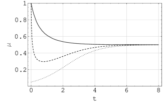
Figure 1: Evolution of the purity of various Gaussian states in a channel with $\mu_{\infty}=0.5$ and $r_{\infty}=0$. The continuous line refers to an initial pure coherent state ($\mu_{0}=1$, $r_{0}=0$), the dashed line refers to a squeezed vacuum ($\mu_{0}=1$, $r_{0}=1.5$) while the dotted line refers to a thermal state with $\mu_{0}=0.05$ and $r_{0}=0$.

The optimal evolution of purity, plotted in Fig. 1, is simply obtained by inserting $r_{0}=r_{\infty}=0$ in Eq. (36).

For an initial squeezed input with squeezing parameter $r_{0}$ in a thermal bath with $r_{\infty}=0$ (or, more generally, for an initial state with relative squeezing $r_{0}-r_{\infty}\neq 0$) the purity $\mu(t)$ may display a local minimum. The condition for the appearance of such a minimum can be simply derived by differentiating Eq. (36) and turns out to be $r_{0}>\max\left[\mu_{0}/\mu_{\infty},\mu_{\infty}/\mu_{0}\right]$; the time $t_{min}$ at which the minimum is attained can be exactly determined as

$$t_{min}=-\frac{1}{\gamma}\ln\left[\frac{\frac{\mu_{0}}{\mu_{\infty}}-\cosh(2r_{0})}{\frac{\mu_{0}}{\mu_{\infty}}+\frac{\mu_{\infty}}{\mu_{0}}-2\cosh(2r_{0})}\right]\;.$$ (39)

The time $t_{min}$ provides a good characterization of the decoherence time of the squeezed state: during the initial steep fall of the purity the coherence and the information contained in the initial state are irreversibly spread in the environmental modes. The subsequent revival of the purity is just a result of the driving of the state of the system towards the (asymptotically reached) environmental one.

Concerning the nonclassical depth, the smallest eigenvalue $u$ of a single mode Gaussian state is simply found in terms of $\mu$, $r$ and $\varphi$ as $u=\,{\rm e}^{-2r}/(2\mu)$. Inserting such a result into Eq. (16) gives the following equation for the non classical depth $\tau$ of a single mode Gaussian state

$$\tau=\max\left[\frac{1-\frac{{\rm e}^{-2r}}{\mu}}{2},0\right]\;.$$ (40)

Let us define the quantity $\kappa(t)$ as

$$\kappa(t)=\frac{\cosh(2r_{0})}{\mu_{0}}\,{\rm e}^{-\gamma t}+\frac{\cosh(2r_{\infty})}{\mu_{\infty}}\left(1-{\rm e}^{-\gamma t}\right)\,.$$

Notice that $\kappa$ is an increasing function of $r_{0}$ and a decreasing function of $\mu_{0}$. After some algebra, Eqs. (37) and (40) yield the following result for the exact time evolution of the nonclassicality of a single mode Gaussian state

$$\tau(t)=\frac{1-\kappa(t)+\sqrt{\kappa(t)^{2}-\frac{1}{\mu(t)^{2}}}}{2}\,.$$ (41)

Such a function increases with both $\mu(t)$ and $\kappa(t)$. The choice of the input phase of the squeezing which maximizes $\tau(t)$ at any time is again $\varphi_{0}=\varphi_{\infty}+\pi/2$, maximizing the purity. The maximization of $\tau(t)$ in terms of the other parameters of the initial state is the result of the competition of two different effects. Let us consider $r_{0}$: on the one hand a squeezing parameter $r_{0}$ matching the squeezing $r_{\infty}$ maximizes the purity thus delaying the decrease of $\tau(t)$; on the other hand, a bigger value of $r_{0}$ obviously yields a greater initial $\tau(0)$. However the numerical analysis, summarized in Fig. 2, unambiguously shows that, in non squeezed baths, the nonclassical depth increases with increasing squeezing $r_{0}$ and purity $\mu_{0}$, as one should expect.

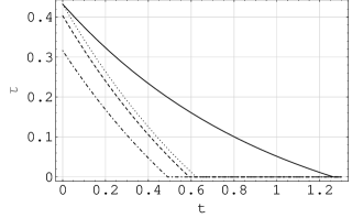
Figure 2: Evolution of the nonclassicality $\tau$ in various channels with $\mu_{\infty}=0.5$. The dotted and the continuous lines refer to an initial squeezed vacuum ($\mu_{0}=1$, $r_{0}=1$) evolving, respectively, in a non squeezed channel (dotted line) and in a channel with $r_{\infty}=0.2$ (continuous line). The dotted line refers to an initial state with $\mu_{0}=0.7$ and $r_{0}=1$ and the dot-dashed line to an initial state with $\mu_{0}=1$ and $r_{0}=0.5$.

5 Schrödinger cats

We consider now the following coherent normalized superposition of single mode displaced squeezed states

$$|\beta_{0},\theta\rangle\equiv\frac{|\beta_{0}\rangle+\;{\rm e}^{i\theta}|-\beta_{0}\rangle}{\sqrt{2+2\cos(\theta)\;{\rm e}^{-2\|X_{0}\|^{2}}}}\>,$$ (42)

where $|\beta_{0}\rangle=S_{r_{0},0}D_{X_{0}}|0\rangle$, and address its evolution under the master equation (22). The choice of a null phase in the operator $S_{r_{0},0}$ is just a reference choice for phase space rotations.

This state is a relevant instance of cat-like state, i.e. of coherent superposition of pure quantum states, whose macroscopic extension has been invoked by Schrödinger to illustrate some of the counterintuitive features of quantum mechanics [45]. More recently, the seminal proposal by Yurke and Stoler [46], besides spurring a great amount of theoretical work aimed at optimizing the generation of cat-like states [47], lead to the experimental realization of mesoscopic ($\|X_{0}\|\simeq 10$) superposition of Gaussian states of the radiation field in cavity QED [48]. The realization of superpositions of Gaussian motional states of trapped particles has been demonstrated as well [49], together with the experimental investigation of their rates of decoherence [50]. On the theoretical side, many efforts have been done to understand and, possibly, suggest methods to control the decoherence of such superpositions [51, 52, 53, 54, 55]. Furthermore, we mention that an accurate analysis, under the ‘quantum jump’ approach, of the decoherence of nonclassical quantum optical states (encompassing both cat-like and number states) can be found in Ref. [56], where it is also shown how nonclassical states may be the result of proper dissipative evolutions. Most of the results here reviewed can be found in Ref. [55].

Let us define the matrices $\boldsymbol{R}=\,{\rm diag}\,(\,{\rm e}^{r_{0}},\,{\rm e}^{-r_{0}})$ (corresponding to the action of $S_{r_{0},0}$ on the $2$-dimensional phase space), and $\boldsymbol{\sigma}_{0}=1/2\boldsymbol{R}^{2}$. The Wigner function associated to the state $|\beta_{0}\rangle$ reads

$$W_{\beta_{0},\theta}(X) = \frac{1}{4\pi(1+\cos(\theta)\,\mathrm{e}^{-\|X_{0}\|^{2}})\sqrt{{\rm Det}\,\boldsymbol{\sigma}_{0}}}$$ (43)

$$\times\left[\,\mathrm{e}^{-\frac{1}{2}(X^{T}-X_{0}^{T}{\bf R})\boldsymbol{\sigma}_{0}^{-1}(X-{\bf R}X_{0})}\right.+\left.\,\mathrm{e}^{-\frac{1}{2}(X^{T}+X_{0}^{T}{\bf R})\boldsymbol{\sigma}_{0}^{-1}(X+{\bf R}X_{0})}\right.$$

$$+\left.\,\mathrm{e}^{-\|X_{0}\|^{2}}\left(\,\mathrm{e}^{-\frac{1}{2}(X^{T}-iX_{0}^{T}\omega{\bf R})\boldsymbol{\sigma}_{0}^{-1}(X+i{\bf R}\omega X_{0})+i\theta}+c.c.\right)\right]\;,$$

consisting in the two Gaussian peaks at the phase space points $X_{0}$ and $-X_{0}$, linked in phase space by the oscillating interference terms. Obviously, this Wigner function is non positive. However, formally, such a function is just the sum of four displaced Gaussian terms. The linearity of the considered dissipative evolution permits to simply solve the evolution of the cat state, by following the evolution of its four Gaussian terms according to Eqs. (31, 32). One gets

$$\begin{split}W_{\beta_{0},\theta}(X)=&\frac{1}{4\pi(1+\cos(\theta)\,\mathrm{e}^{-\|X_{0}\|^{2}})\sqrt{{\rm Det}\,\boldsymbol{\sigma}(t)}}\\ &\times\left[\,\mathrm{e}^{-\frac{1}{2}(X^{T}-\,{\rm e}^{-\frac{\gamma}{2}t}X_{0}^{T}{\bf R})\boldsymbol{\sigma}(t)^{-1}(X-\,{\rm e}^{-\frac{\gamma}{2}t}{\bf R}X_{0})}\right.\\ &+\left.\,\mathrm{e}^{-\frac{1}{2}(X^{T}+\,{\rm e}^{-\frac{\gamma}{2}t}X_{0}^{T}{\bf R})\boldsymbol{\sigma}(t)^{-1}(X+\,{\rm e}^{-\frac{\gamma}{2}t}{\bf R}X_{0})}\right.\\ &+\left.\,\mathrm{e}^{-\|X_{0}\|^{2}}\left(\,\mathrm{e}^{-\frac{1}{2}(X^{T}-i\,{\rm e}^{-\frac{\gamma}{2}t}X_{0}^{T}\omega{\bf R})\boldsymbol{\sigma}(t)^{-1}(X+i\,{\rm e}^{-\frac{\gamma}{2}t}{\bf R}\omega X_{0})+i\theta}+c.c.\right)\right]\;,\end{split}$$ (44)

where $\boldsymbol{\sigma}(t)$ is given by Eq. (31) with $\boldsymbol{\sigma}_{0}$ defined above.

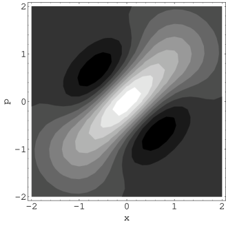
(a)

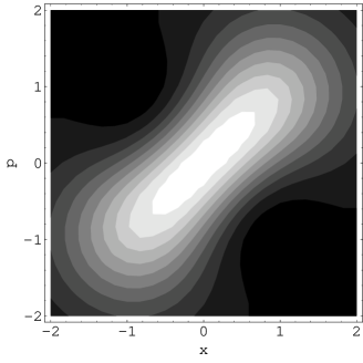
(b)

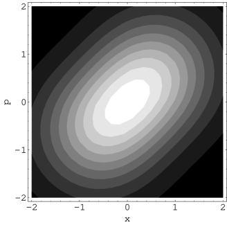
(c)

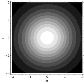
(d)

Figure 3: Evolution in phase space of the Wigner function of an initial non squeezed cat-like state with $X_{0}^{T}=(1\;1)$ and $\theta=0$ in a thermal channel with $\mu_{\infty}=0.5$ at times $t=0$ (a), $t=\gamma^{-1}/2$ (b), $t=\gamma^{-1}$ (c) and $t=4\gamma^{-1}$ (d). Darker colors stand for lower values, the scale of each plot is normalized. The negative lobes (in which the Wigner function takes negative values), evident in subfigure (a) are already disappeared in subfigure (b). Actually, the positive time $t_{nc}$ of such a reservoir is $t_{nc}\simeq 0.4\gamma^{-1}$ (see Eq. (34)).

Figure 3 provides a relevant example of dissipation of a cat state in a thermal environment, isotrope in phase space. The negative part $\xi$ of the Wigner function reaches the value $0$ at a time $t_{nc}\simeq 0.4\gamma^{-1}$, in agreement with Eq. (34). As already mentioned, this time is feature of the bath and does not depend on the initial pure (non Gaussian) state.

The exact analytical expression of the purity of the evolving superposition is easily determined by Gaussian integrations, according to Eq. (17)

$$\mu_{\beta_{0},\theta}(t) = \left(8(1+\cos(\theta)\,{\rm e}^{-\|X_{0}\|^{2}})^{2}\sqrt{{\rm Det}\,\boldsymbol{\sigma}(t)}\right)^{-1}$$ (45)

$${\times\Bigg{[}2}\left(1+{\rm e}^{-\,{\rm e}^{-\gamma t}X_{0}^{T}{\bf S}(t)X_{0}}\right)+2\,{\rm e}^{-2\|X_{0}\|^{2}}\left(\cos(2\theta)+{\rm e}^{\,{\rm e}^{-\gamma t}X_{0}^{T}{\bf T}(t)X_{0}}\right)$$

$${+4\,{\rm e}}^{-\|X_{0}\|^{2}}\cos(\theta)\left({\rm e}^{-\,{\rm e}^{-\gamma t}X_{0}^{T}\boldsymbol{J}X_{0}\,{\rm Tr}[\boldsymbol{J}\boldsymbol{S}(t)]^{*}/4}+c.c.\right)\Bigg{]}\,,$$

with

$${\bf S}(t)\equiv{\bf R}\boldsymbol{\sigma}(t)^{-1}{\bf R}\,,\quad{\bf T}(t)\equiv({\rm Det}\,\boldsymbol{\sigma})^{-1}{\bf S}(t)^{-1}\,,\quad{\bf J}\equiv\left(\begin{array}[]{cc}1&i\\ i&-1\end{array}\right)\,.$$ (46)

Eq. (45) shows that the decoherence rate increases with the ‘dimension’ of the cat, quantified by $\|X_{0}\|$; in the limiting instance $X_{0}=0$, Eq. (45) reduces to Eq. (36) for an initial squeezed vacuum, which decoheres more slowly than the equally squeezed cat-like states. Moreover, in general, the terms depending on the coherent phase $\theta$ are suppressed by exponential terms of the form $\exp(-\|X_{0}\|^{2})$, so that the decoherence rate in terms of the purity is only slightly influenced by the choice of $\theta$. Examples of decoherence of cat states can be seen in Fig. 4.

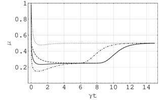
Figure 4: Evolution of the purity of initial cat-like states. The asymptotic purity of the channel is $\mu_{\infty}=0.5$. The dotted line refers to a cat state with $X_{0}^{T}=(1,\;1)$ in a non squeezed channel. The dashed and the continuous lines refer to an initial non squeezed cat with $X_{0}^{T}=(100,\;100)$ evolving in a non squeezed channel and in a channel with $r_{\infty}\simeq 0.88$ and $\varphi_{\infty}=-\pi/8$. The dot-dashed line refers to an initial state with $X_{0}^{T}=(10,\;10)$ and $r_{0}=2$ evolving in a non squeezed channel.

In all the instances the purity displays a fast initial fall, during which all the coherence and the information of the pure cat-like state are lost. The typical time scale in which the minimum of the purity is attained is in good agreement with the estimate $t_{dec}=\gamma^{-1}/2\|X_{0}\|^{2}$, holding for the decoherence time of a cat state in a thermal bath [50]. As can be shown analytically [55], the phase space direction of the cat, determined by the angle $\xi_{0}=\arctan(x_{0}/p_{0})$, providing the maximal delay of decoherence at short times (i.e. for $\gamma t\simeq 1$) is given by $\xi_{0}=\varphi_{0}+\pi/2$ for a squeezed cat in a non squeezed bath or, equivalently, by $\xi_{0}=\varphi_{\infty}$ for a non squeezed cat in a squeezed bath. These two instances are, as already noted, unitarily equivalent. In general, the evolution of the purity of an initial state in a squeezed reservoir is identical to the one of the counter-squeezed initial state in a thermal reservoir. Therefore, the same protection against decoherence granted by squeezing the bath can be achieved by orthogonally squeezing the initial state. Indeed, with the optimal, previously discussed, locking of the optical phase, an optimal value of the squeezing $r_{0}$ maximizing the purity in non squeezed baths does exist. As illustrated by Fig. 5, squeezing the initial cat (or the bath) can provide a significant delay of the complete decoherence of the cat state, better preserving the interference fringes in phase space.

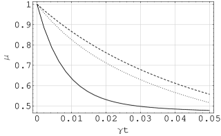
Figure 5: Comparison between the evolution at short times (i.e. for $\gamma t_{dec\simeq 1}$) of the purity of an initial non squeezed cat (continuous line) and that of squeezed cats with optimal choice of the optical phase. In all instances $X_{0}^{T}=(4,\;4)$, $\mu_{\infty}=0.5$ and $\theta=0$. The dashed line refers to a cat state with $r_{0}=1$, whereas the dotted line refers to a state with $r_{0}=1.5$. The decoherence time of such cats can be estimated as $t_{dec}\simeq 0.03\gamma^{-1}$, in good agreement with the decrease of purtiy of the non squeezed cat. The remarkable delay of decoherence induced by squeezing the cat can be appreciated, especially at $t\simeq t_{dec}$.

6 Number states

As a last example of single mode state we quantify the decoherence of number states $|n\rangle\langle n|$. Such states can be considered as probe of fundamental quantum mechanical features and are also required in several quantum communications tasks [57, 58]. Different methods for the generation of Fock states have been proposed, both for traveling-wave and cavity fields. For traveling-wave fields, these methods are principally based on tailored nonlinear interactions [59], conditional measurements [60], state filtering [61] or state engineering [62]. A further possibility to generate number states with high fidelities by atom-field interactions in high-$Q$ cavities has been recently suggested [63]. The actual experimental generation in quantum optical settings seems to be at hand, by both deterministic [64, 65] and probabilistic (‘post-selective’) schemes [66] (and the techniques to realize such states for motional degrees of freedom are well mastered [67]), even if the numerical analysis suggests that environmental decoherence could still hamper the very possibility of generating pure number states [68]. These reasons motivated an accurate investigation of the decoherence rate of number states, carried out in Ref. [69]. We review such results, adding the analysis of the nonclassicality of the evolving states.

The characteristic function $\chi_{n}$ associated to the state $|n\rangle\langle n|$ is promptly found and reads [7]

$$\chi_{n}(X)=\langle n|D_{\alpha}|n\rangle=\,{\rm e}^{-\frac{\|X\|^{2}}{2}}L_{n}(\|X\|^{2})\,,$$ (47)

where $L_{n}$ is the Laguerre polynomial of order $n$: $L_{n}(x)=\sum_{m=0}^{n}\frac{(-x)^{m}}{m!}{n\choose m}$. So that, exploiting Eq. (29), one at once finds the evolution of such an initial state in the channel

$$\chi_{n}(t)=L_{n}\left(\frac{\|X\|^{2}}{2}\,{\rm e}^{-\gamma t}\right)\,{\rm e}^{-\frac{1}{2}X^{T}\boldsymbol{\sigma}(t)X}\,,$$ (48)

with

$$\boldsymbol{\sigma}(t)=\frac{\mathbbm{1}}{2}\,{\rm e}^{-\gamma t}+\boldsymbol{\sigma}_{\infty}(1-\,{\rm e}^{-\gamma t})\;.$$ (49)

According to Eq. (17) one can then determine the purity $\mu_{n}(t)$ of the evolving number state [70]

$$\mu_{n}(t)=\,{\rm e}^{\gamma t}\int_{0}^{\infty}\,{\rm e}^{-\xi s}L_{n}(s)I_{0}\left(\frac{|\sinh(2r_{\infty})|}{2\mu_{\infty}}(\,{\rm e}^{\gamma t}-1)s\right)\,{\rm d}s\,,$$ (50)

where $I_{0}(x)=J_{0}(ix)=\sum_{k=0}^{\infty}\frac{x^{2k}}{(2^{k}k!)^{2}}$ is the zero order modified Bessel function of the first kind and

$$\xi=\frac{{\rm e}^{\gamma t}+\mu_{\infty}-1}{\mu_{\infty}}\;.$$

For a thermal channel, with $r_{\infty}=0$, such an expression can be further simplified to achieve an exact analytical expression for the purity, yielding [70]

$$\mu_{n}(t)=\,{\rm e}^{\gamma t}\frac{(\xi-2)^{2}}{\xi^{n+1}}P_{n}\left(1+\frac{2}{\xi^{2}-2\xi}\right)\,,$$ (51)

where $P_{n}$ is the Legendre polynomial of order $n$: $P_{n}(x)=\frac{1}{2^{n}n!}\frac{{\rm d}^{n}}{{\rm d}\,x^{n}}(x^{2}-1)^{n}$. Again, we point out that the squeezing of the bath has the same effect on the purity as the counter squeezing of the initial number state, amounting to consider a ‘squeezed number state’. The numerical analysis of Eq. (50) at short times (for $\gamma t\lesssim 1$) shows that $\mu_{n}(t)$ is a decreasing function of $r_{\infty}$: the squeezing of the bath does not help to preserve the coherence of number states. Also, the purity at any given time is a decreasing function of $n$: number states of higher order are more fragile and decoheres faster.

Let us now deal with the evolution of the negative part $\xi$ of a number state $|n\rangle$, quantifying the decoherence effect on the nonclassical features of the state. The initial value of such a quantity increases with increasing $n$ (higher order number states are regarded as ‘less classical’ by this indicator). Subsequently, during the dissipation in the bath, the negative part $\xi$ decreases up to a time $t_{nc}$ – determined by Eq. (34) – at which it reaches the values $0$ and the nonclassical features of the state related to $\xi$ are erased. Interestingly, a direct determination of the time $t_{nc}$ can be easily provided for the relevant instance of number states evolving in non squeezed thermal baths (with $r_{\infty}=0$). In such a case, the spherically symmetric characteristic function of Eq. (48) for $r_{\infty}=0$ can be Fourier transformed to get the Wigner function $W_{n}(t)$

$$W_{n}(t)=\frac{\eta(t)^{n}}{\pi\zeta(t)^{n+1}}\,{\rm e}^{-\frac{\|X\|^{2}}{\zeta(t)}}L_{n}\left[\frac{-2\,{\rm e}^{-\gamma t}\|X\|^{2}}{\zeta(t)\eta(t)}\right]\,,$$ (52)

with

$$\zeta(t)=\frac{1}{\mu_{\infty}}\left[1-(1-\mu_{\infty})\,{\rm e}^{-\gamma t}\right]\quad{\rm and}\quad\eta(t)=\frac{1}{\mu_{\infty}}\left[1-(1+\mu_{\infty})\,{\rm e}^{-\gamma t}\right]\,.$$

Since Laguerre polynomials of any order have positive roots and are always positive for negative arguments, Eq. (52) implies that the time $t_{nc}$ is determined by the condition $\eta(t_{nc})=0$, yielding $t_{nc}=\gamma^{-1}\ln(1+\mu_{\infty})$. This result is just a specific instance of Eq. (34), which can be applied at any pure non Gaussian initial state. It can also be found in Ref. [71], where the remarkable independence of the time $t_{nc}$ on the order $n$ of the number state had already been stressed.

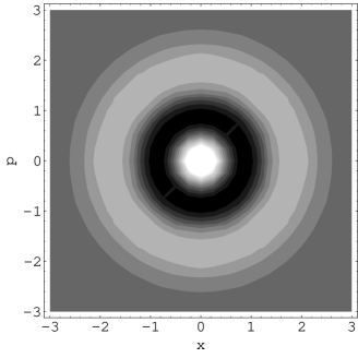
(a)

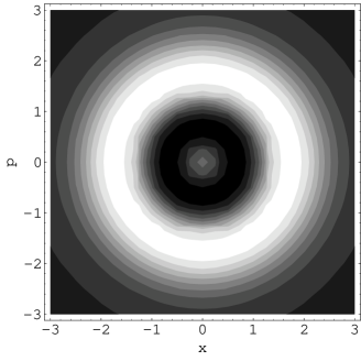
(b)

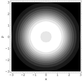
(c)

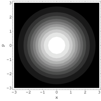
(d)

Figure 6: Evolution in phase space of the Wigner function of the initial number state $|2\rangle$ in a thermal channel with $\mu_{\infty}=0.5$ at times $t=0$ (a), $t=\gamma^{-1}/4$ (b), $t=\gamma^{-1}$ (c) and $t=1.5\gamma^{-1}$ (d). Darker colors stand for lower values, the scale of each plot is normalized. The time $t_{nc}$, at which the Wigner function of this state gets positive is $t_{nc}\simeq 0.4\gamma^{-1}$. As can be seen, at $t=\gamma^{-1}$, the central minimum deriving from the initial negative zone is still evident, but takes only positive values.

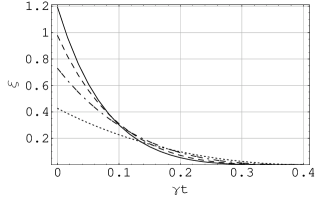
Figure 7: Time evolution of the negative part $\xi$ of the number states $|1\rangle$ (dotted line), $|2\rangle$ (dot-dashed line), $|3\rangle$ (dashed line) and $|4\rangle$ (continuous line), in a thermal reservoir with $\mu_{\infty}=0.5$. For such a reservoir, the Wigner function gets positive at $t_{nc}\simeq 0.4\gamma^{-1}$.

The evolution in phase space of the Wigner function of Eq. (52) is showed in Fig. 6. Fig. 7 shows the time dependence of the negative part $\xi$, numerically integrated for the first four number states in a thermal reservoir. Even though the initial negative part increases with increasing $n$, the quantity $\xi(t)$ is not increasing with $n$ at any time: indeed, lower order states better preserve such nonclassical features when approaching the time $t_{nc}$ (which, we recall once again, does not depend on the initial pure non Gaussian state).

A relevant instance to exemplify the decoherence of number states is provided by the coherent normalized superposition $|\psi_{01}\rangle=(|0\rangle+\,{\rm e}^{i\vartheta}|1\rangle)/\sqrt{2}$, constituting a microscopic Schrödinger cat. The characteristic function $\chi_{01}$ of this state is simply found [7]

$$\chi_{01}(\alpha)=\frac{{\rm e}^{-\frac{|\alpha|^{2}}{2}}}{2}\left[2-\,{\rm e}^{-\gamma t}|\alpha|^{2}-\,{\rm e}^{-\frac{\gamma t}{2}}(\alpha^{*}\,{\rm e}^{-i\vartheta}-\alpha\,{\rm e}^{i\vartheta})\right].$$ (53)

Inserting $\chi_{01}$ as the initial condition in Eq. (29) and performing the integration of Eq. (17) yields, for the purity of the initial cat-like state evolving in the channel

$$\mu_{01}(t,r) = 4\nu-\,{\rm e}^{-2\gamma t}\frac{\nu^{2}}{2\mu_{\infty}}\Big{(}\mu_{\infty}+(\,{\rm e}^{\gamma t}-1)(\cosh(2r)$$ (54)

$$+ \cos(2\vartheta-2\varphi)\sinh(2r))\Big{)}$$

$$+ \,{\rm e}^{-4\gamma t}\frac{\nu^{5}}{2\mu_{\infty}^{2}}\Big{(}4\mu_{\infty}^{2}+8(\,{\rm e}^{\gamma t}-1)\mu_{\infty}\cosh(2r)$$

$$+ (\,{\rm e}^{\gamma t}-1)^{2}(3\cosh(4r)+1)\Big{)}$$

where

$$\nu=\bigg{[}\frac{1}{\mu_{\infty}^{2}}\left(1-{\rm e}^{-\gamma t}\right)^{2}\,+\,{\rm e}^{-2\gamma t}+2\frac{1}{\mu_{\infty}}\cosh(2r)\bigg{]}^{-1/2}$$ (55)

is the purity of an initial vacuum in the channel, found in Sec. 4. Eq. (54) shows that the evolution of the coherent superposition is sensitive to the phase $\varphi$ of the bath. It is straightforward to see that the optimal choice maximizing purity at any given time is provided by $\vartheta=\varphi+\pi/2$. Fixing such a choice, we have numerically analyzed the dependence of $\mu_{01}$ on the squeezing parameter $r_{\infty}$. For small $r_{\infty}$ the purity $\mu_{01}$ increases with $r$. The optimal choice for $r_{\infty}$ depends on time, for $\gamma t=0.5$ it turns out to be $r\simeq 0.28$. The relative increase in purity for several choices of the squeezing parameter $r_{\infty}$ is plotted in Fig. 8 as a function of time. It is interesting to compare this analysis of decoherence with the one previously carried out for Gaussian catlike states. Indeed, notwithstanding the deeply quantum nature of a superposition of number states, its decoherence rate is comparatively slow. Actually, the purity of the considered superposition in a thermal channel reaches the asymptotic value of the channel, after the initial decrease, in a time $t\simeq 0.5\gamma^{-1}$. Such a time length corresponds to the decoherence time $t_{dec}$ of a superposition of two Gaussian terms displaced in phase space of only one coherent photon (in opposite directions with respect to the origin, i.e. with $\|X_{0}\|^{2}=1$ in the notation of the previous section). Despite the relevant intrinsic differences between these two kinds of Schrödinger cat states, their decoherence is basically driven by the same process, due to the entanglement of the system with the environmental degrees of freedom.

We remark that the time of decoherence can be much shorter of the time characterizing the energy relaxation [31, 50], which constitutes however a strict upper bound on the former. This fact is a manifestation of a general feature of quantum mechanics. Nonclassical superpositions decohere on a time scale of the photon lifetime in the channel, regardless of the other parameters: once a single photon is added or lost, all the information contained in the original state leaks out to the environment. This can be understood, euristically, by considering the action of the annihilation operators $a$ which, in general, modifies the coherent phase of the superposition. Therefore, as soon as the probability of losing a photon reaches $0.5$, the original superposition turns into an incoherent mixtures of states with different phase, whose interference terms cancel out each other [56, 72]. No coherent behaviour can survive such a dissipative process and be afterwards revealed by interferometry.

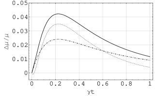
Figure 8: The relative increase in purity, defined by $\Delta\mu/\mu=(\mu_{01}(t,r)-\mu_{01}(t,0))/\mu_{01}(t,0)$, as a function of time during the evolution of the superposition $|\psi_{01}\rangle$ in Gaussian channels. The optimal condition $\vartheta=\varphi+\pi/2$ is always assumed, while $\mu_{\infty}=0.25$. The solid line refers to a bath with $r=0.28$, close to the optimal value; the dotted line refers to a bath with $r=0.4$ and the dot–dashed line refers to a bath with $r=0.1$.

7 Two-mode Gaussian states

Two-mode Gaussian states are the simplest example of continuous variable bipartite states. Their decoherence under the quantum optical master equation can be therefore characterized also by investigating the evolution of the correlations between the two modes of the systems. In particular, the decay of quantum correlations, i.e. of the entanglement, quantified by the logarithmic negativity, may be adopted as an indicator of decoherence. Due to their clear interest, concerning both applications in quantum information and the study of fundamental features of entanglement, the behaviour of two-mode Gaussian states under non unitary evolutions has attracted a remarkable theoretical interest in later years [73, 74, 75, 76, 77, 78, 79, 80]. We review here the results of Ref. [80]; moreover, we consider the instance of different couplings to the bath and provide a detailed study of the evolving nonclassical depth.

Before addressing the analysis of their decoherence in detail, let us recall some basic facts about two-mode Gaussian states. The $4\times 4$ covariance matrix $\boldsymbol{\sigma}$ shall be conveniently written in terms of the three $2\times 2$ submatrices $\boldsymbol{\alpha}$, $\boldsymbol{\beta}$, $\boldsymbol{\gamma}$

$$\boldsymbol{\sigma}\equiv\left(\begin{array}[]{cc}\boldsymbol{\alpha}&\boldsymbol{\gamma}\\ \boldsymbol{\gamma}^{T}&\boldsymbol{\beta}\end{array}\right)\,.$$ (56)

The CM $\boldsymbol{\sigma}$ can be put into the so called standard form $\boldsymbol{\sigma}_{sf}$ through a local symplectic operation $S_{l}=S_{1}\oplus S_{2}$

$$S_{l}^{T}\boldsymbol{\sigma}S_{l}=\boldsymbol{\sigma}_{sf}\equiv\left(\begin{array}[]{cccc}a&0&c_{1}&0\\ 0&a&0&c_{2}\\ c_{1}&0&b&0\\ 0&c_{2}&0&b\end{array}\right)\;.$$ (57)

In what follows, let us suppose $|c_{2}|\geq|c_{1}|$. States whose standard form fulfills $a=b$ are said to be symmetric. Let us recall that any pure state is symmetric and fulfills $c_{1}=-c_{2}=\sqrt{a^{2}-1/4}$. The correlations $a$, $b$, $c_{1}$, and $c_{2}$ are determined by the four local symplectic invariants ${\rm Det}\boldsymbol{\sigma}=(ab-c_{1}^{2})(ab-c_{2}^{2})$, ${\rm Det}\boldsymbol{\alpha}=a^{2}$, ${\rm Det}\boldsymbol{\beta}=b^{2}$, ${\rm Det}\boldsymbol{\gamma}=c_{1}c_{2}$. Therefore, the standard form corresponding to any covariance matrix is unique (up to a common sign flip in the $c_{i}$’s).

The $Sp_{(4,{\mathbb{R}})}$ invariants ${\rm Det}\boldsymbol{\sigma}$ and $\Delta(\boldsymbol{\sigma})={\rm Det}\boldsymbol{\alpha}+\,{\rm Det}\boldsymbol{\beta}+2\,{\rm Det}\boldsymbol{\gamma}$ permit to explicitly express Ineq. (9) in terms of second moments

$$\Delta(\boldsymbol{\sigma})\leq\frac{1}{4}+4\,{\rm Det}\boldsymbol{\sigma}\;$$ (58)

and determine the symplectic spectrum $\{\nu_{\mp}\}$ of $\boldsymbol{\sigma}$, according to [24]

$$2\nu_{\mp}^{2}=\Delta(\boldsymbol{\sigma})\mp\sqrt{\Delta(\boldsymbol{\sigma})^{2}-4\,{\rm Det}\,\boldsymbol{\sigma}}\;.$$

A relevant subclass of Gaussian states we will make use of is constituted by the two–mode squeezed thermal states. Let $S_{r}=S_{12,r,0}$ be the two-mode squeezing operator between the modes $1$ and $2$ with real squeezing parameter $r$ and let $\nu_{\mu}$ be the tensor product of identical thermal states of global purity $\mu$, with CM $\boldsymbol{\nu}_{\mu}=1/(2\sqrt{\mu}){\mathbbm{1}}$. Then, for a two-mode squeezed thermal state ${\xi}_{\mu,r}$ we can write ${\xi}_{\mu,r}=S_{r}{\nu}_{\mu}S_{r}^{{\dagger}}$. The CM $\boldsymbol{\xi}_{\mu,r}$ of $\xi_{\mu,r}$ is a symmetric standard form satisfying

$$a=\frac{\cosh 2r}{2\sqrt{\mu}}\;,\quad c_{1}=-c_{2}=\frac{\sinh 2r}{2\sqrt{\mu}}\,.$$ (59)

In the instance $\mu=1$ one recovers the pure two–mode squeezed vacuum states. Two–mode squeezed states are endowed with remarkable properties related to entanglement [81], in particular they are the maximally entangled states for given marginal and global purities [16, 17].

We recall that the necessary and sufficient separability criterion for two-mode Gaussian states is positivity of the partially transposed density matrix (“PPT criterion”) [26]. It can be easily seen from the definition of $W(X)$ that the action of partial transposition amounts, in phase space, to a mirror reflection of one of the four canonical variables. In terms of the $Sp_{4,\mathbb{R}}$ invariants, this results in changing the invariant $\Delta(\boldsymbol{\sigma})$ into $\tilde{\Delta}({\boldsymbol{\sigma}})=\Delta(\tilde{\boldsymbol{\sigma}})=\,{\rm Det}\,\boldsymbol{\alpha}+\,{\rm Det}\,\boldsymbol{\beta}-2\,{\rm Det}\,\boldsymbol{\gamma}$. Now, the symplectic eigenvalues $\tilde{\nu}_{\mp}$ of the partially transposed CM $\tilde{\boldsymbol{\sigma}}$ read

$$\tilde{\nu}_{\mp}=\sqrt{\frac{\tilde{\Delta}(\boldsymbol{\sigma})\mp\sqrt{\tilde{\Delta}(\boldsymbol{\sigma})^{2}-4\,{\rm Det}\,\boldsymbol{\sigma}}}{2}}\,.$$ (60)

The PPT criterion then reduces to a simple inequality that must be satisfied by the smallest symplectic eigenvalue $\tilde{\nu}_{-}$ of the partially transposed state

$$\tilde{\nu}_{-}\geq\frac{1}{2}\>,$$ (61)

which is equivalent to

$$\tilde{\Delta}(\boldsymbol{\sigma})\leq 4\,{\rm Det}\,\boldsymbol{\sigma}+\frac{1}{4}\;.$$ (62)

The above inequalities imply ${\rm Det}\,\boldsymbol{\gamma}=c_{1}c_{2}<0$ as a necessary condition for a two–mode Gaussian state to be entangled. The quantity $\tilde{\nu}_{-}$ encodes all the qualitative characterization of the entanglement for arbitrary (pure or mixed) two–modes Gaussian states. Note that $\tilde{\nu}_{-}$ takes a particularly simple form for entangled symmetric states, whose standard form has $a=b$

$$\tilde{\nu}_{-}=\sqrt{(a-|c_{1}|)(a-|c_{2}|)}\;.$$ (63)

The logarithmic negativity $E_{{\cal N}}$ of two–mode Gaussian states is a simple function of $\tilde{\nu}_{-}$, which is thus itself an (increasing) entanglement monotone; one has in fact [17]

$$E_{{\cal N}}(\boldsymbol{\sigma})=\max\left\{0,-\ln{2\tilde{\nu}_{-}}\right\}\>.$$ (64)

This is a decreasing function of the smallest partially transposed symplectic eigenvalue $\tilde{\nu}_{-}$, quantifying the amount by which Inequality (61) is violated. Thus, for our aims, the eigenvalue $\tilde{\nu}_{-}$ completely qualifies and quantifies the quantum entanglement of a two–mode Gaussian state $\boldsymbol{\sigma}$.

The smallest eigenvalue $u$ of $\boldsymbol{\sigma}_{sf}$ (which determines the nonclassical depth $\tau$ according to Eq. (16)) is easily determined

$$2u=a+b-\sqrt{(a-b)^{2}+4c_{2}^{2}}\;,$$ (65)

reducing to $u=a-|c_{2}|$ for symmetric states and to $u=\,{\rm e}^{-2r}/(2\sqrt{\mu})$ for two-mode squeezed thermal states.

The evolution of two-mode Gaussian states in the noisy channel is described by Eq. (32) with $n=2$. The channel is completely determined by the quantities $\mu_{i\infty}$, $r_{i\infty}$, $\varphi_{i\infty}$ and $\gamma_{i}$, for $i=1,2$. Notice that, if $\gamma_{1}\neq\gamma_{2}$, then a change in the values of the couplings to the bath $\gamma_{i}$’s does not reduce to a rescaling of time and may significantly affect the evolution of the relevant quantities in the channel. For the study of the entropic measures and of correlations, we will restrict to initial states in the standard form of Eq. (57), with no loss of generality since all such quantities are invariant under local unitary operations. On the other hand, the nonclassical depth $\tau$ is not invariant under such operations. Determining the evolution of such a quantity in the general instance is slightly more involved. For the sake of simplicity, we will study such evolution in relevant instances, which can be conveniently handled and illustrate the general behaviour of the nonclassical indicator. Henceforth, we will set $\varphi_{1\infty}=0$ as a reference choice for phase space rotations.

Exploiting the results we have just reviewed, together with the general definitions of Sec. 2, we can determine the exact evolution in the channel of the entropic measures $\mu$ and $S_{V}$, and of the quantum and total correlations, respectively quantified by $E_{\cal N}$ and $I$. In Appendix A we provide the explicit expression of the time dependent terms, allowing to compute such evolutions, in the instance of equal couplings: $\gamma_{1}=\gamma_{2}=\gamma$.

As for the evolution of the purity $\mu$ and of the von Neumann entropy $S_{V}$ – whose decrease quantifies the information which the composite two mode state ‘as a whole’ loses by interacting with the environment – some analytical statements can be done. It can be shown by means of a variational approach [38] that the purity of a given channel of the form of Eq. (32) is maximized by an uncorrelated state (with $c_{1}=c_{2}=0$ in our notation). Its maximization is therefore achieved by the (obviously separable) product of two ‘countersqueezed’ states, which, as we have seen in Sec. 4 maximizes the local purity relative to the two single-mode channels. The optimal purity evolution reduces therefore to the square of the optimal purity evolution for single mode channels, previously studied. This feature holds for any value of $\gamma_{1}$ and $\gamma_{2}$. An analogous argument can be applied to the von Neumann entropy $S_{V}$ which, we recall, is fully determined by the quantity $\lim_{p\rightarrow 0}\,{\rm Tr}\,\varrho^{p}$. However, so far, the fact that the minimal $S_{V}$ at any given time is achieved by an uncorrelated input has been proved only for $\gamma_{1}=\gamma_{2}$. The numerical analysis, summarized in Fig. 9, remarkably supports the conjecture of the additivity of the minimal output von Neumann entropy also for $\gamma_{1}\neq\gamma_{2}$.

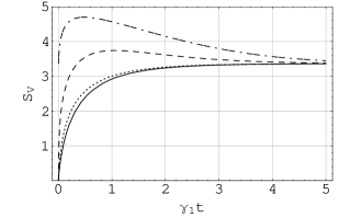
Figure 9: Time evolution of the von Neumann entropy in a thermal channel with $\gamma_{1}=1$, $\gamma_{2}=2$ and $\mu_{1\infty}=\mu_{2\infty}=0.25$. The continuous line refers to the conjectured optimal evolution, achieved by a pure separable input state with $a=b=1/2$ and $c_{1}=c_{2}=0$ in a non squeezed channel; the dotted line refers to a n inital pure two mode squeezed state with $r=0.5$ in the same channel. The dashed and dot-dashed lines refer to a squeezed channel with $r_{1\infty}=r_{2\infty}=1$ and, respectively to an initial pure two mode squeezed state with $r=1$ and an intial thermal two mode squeezed state with $\mu=1/16$ (equal to the asymptotic purity).

We now move to consider the decay of the entanglement between the two modes of the field, i.e. the leaking to the environment of the information contained in quantum correlations between the two modes. Supposing that the couplings to the two baths are equal ($\gamma_{1}=\gamma_{2}=\gamma$) and making use of the separability criterion given by Ineq. (62), one finds that an initially entangled state becomes separable at a certain time $t$ if

$$u\,{\rm e}^{-4\gamma t}+v\,{\rm e}^{-3\gamma t}+w\,{\rm e}^{-2\gamma t}+y\,{\rm e}^{-\gamma t}+z=0\,.$$ (66)

The coefficients $u$, $v$, $w$, $y$ and $z$ are functions of the nine parameters characterizing the initial state and the channel (see App. A). Eq. (66) is an algebraic equation of fourth degree in the unknown $k={\rm e}^{-\gamma t}$. The solution $k_{ent}$ of such an equation closest to one, and satisfying $k_{ent}\leq 1$ can be found for any given initial entangled state. Its knowledge promptly leads to the determination of the “entanglement time” $t_{ent}$ of the initial state in the channel, defined as the time interval after which the initial entangled state becomes separable

$$t_{ent}=-\frac{1}{\gamma}\ln k_{ent}\,.$$ (67)

The entanglement time $t_{ent}$ can be easily estimated for symmetric states (for which $a=b$) evolving in equal thermal baths (i.e. with $\gamma_{1}=\gamma_{2}=\gamma$ and $\mu_{1\infty}=\mu_{2\infty}=\sqrt{\mu_{\infty}}$). In such a case the initally entangled state maintains its symmetric standard form during the time evolution. Recalling that $|c_{1}|\leq|c_{2}|$, we have that Eqs. (61) and (63) provide the following bounds for the entanglement time

$$\ln\left(1+\sqrt{\mu_{\infty}}\frac{2|c_{1}|-2a+1}{1-\sqrt{\mu_{\infty}}}\right)\leq\gamma t_{ent}\leq\ln\left(1+\sqrt{\mu_{\infty}}\frac{2|c_{2}|-2a+1}{1-\sqrt{\mu_{\infty}}}\right)\,.$$ (68)

Note that $\mu_{\infty}$ is the global purity of the asymptotic two mode state. Imposing the additional property $c_{1}=-c_{2}$ amounts to consider standard forms which can be written as squeezed thermal states (see Eqs. 59). For such states, Inequality (68) reduces to

$$t_{ent}=\frac{1}{\gamma}\ln\left(1+\sqrt{\mu_{\infty}}\frac{1-\frac{{\rm e}^{-2r}}{\sqrt{\mu}}}{1-\sqrt{\mu_{\infty}}}\right)\;.$$ (69)

In particular, for $\mu=1$, one recovers the entanglement time of a two–mode squeezed vacuum state in a thermal channel [27, 77, 79]. We point out that two–mode squeezed vacuum states encompass all the possible standard forms of pure Gaussian states.

The results of the numerical analysis of the evolution of the logarithmic negativity for several initial states are reported in Figs. 10 and 11. In general, one can see that a less mixed environment better preserves entanglement by prolonging the entanglement time. More remarkably, Fig. 10 shows that a local squeezing of the two uncorrelated channels does not help to preserve the quantum correlations between the evolving modes. Moreover, as can be seen from Fig. 11, states with greater uncertainties on, say, mode $1$ ($a>b$) better preserves its entanglement if bath $1$ is more mixed than bath $2$ ($\mu_{1\infty}<\mu_{2\infty}$). Fig. 11 also shows that, even for initial non symmetric states, unbalancing the couplings to the two single mode reservoirs (while leaving their average unchanged: $\gamma=(\gamma_{1}+\gamma_{2})/2$) only slightly affects the evolution of the entanglement in the channel; an accurate numerical analysis shows that a greater coupling to the more mixed initial mode (e.g., $\gamma_{1}>\gamma_{2}$ if $a>b$) enhances the preservation of the initial quantum correlations. Also, for symmetric states evolving in squeezed baths, one can see that the entanglement of the initial state is better preserved if the squeezing of the two channels is balanced.

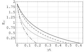
Figure 10: Time evolution of the logarithmic negativity of an initial two mode squeezed thermal state with $\mu=0.8$ and $r=1$ in several channels with $\gamma_{1}=\gamma_{2}=\gamma$. The continuous line refers to a non squeezed bath with $\mu_{1\infty}=\mu_{2\infty}=0.5$ (corresponding to $0.5$ thermal photons); the dotted line correspond to a thermal bath with $\mu_{1\infty}=0.25$ and $\mu_{2\infty}=1$ (with a global asymptotic purity equal to the previous one); the dashed and dot-dashed lines refer to a bath with $\mu_{1\infty}=\mu_{2\infty}=0.5$, $r_{1\infty}=r_{2\infty}=1$ and $\varphi_{2\infty}=0$ ($\varphi_{2\infty}=\pi/4$) for the dashed (dot-dashed) line.

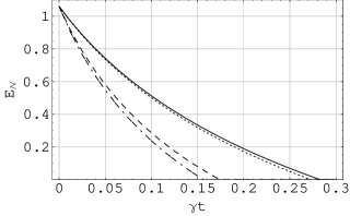
Figure 11: Time evolution of the logarithmic negativity of an inital entangled non symmetric state, obtained from the squeezed thermal one considered in Fig. 10 by adding $0.2$ to the element $a$ of the standard form (added noise on mode $1$ quadratures.) The solid line refers to a bath with $\gamma_{1}=\gamma_{2}=\mu_{1\infty}=\mu_{2\infty}=1$; the dotted line refers to a channel with $\gamma_{1}=0.5$, $\gamma_{2}=1.5$ and $\mu_{1\infty}=\mu_{2\infty}=1$; the dashed (dot-dashed) line refers to a bath with $\gamma_{1}=\gamma_{2}=1$, $\mu_{1\infty}=1/9$ ($\mu_{1\infty}=1$) and $\mu_{2\infty}=1$ ($\mu_{2\infty}=1/9$). The label $\gamma$ is defined by $\gamma=(\gamma_{1}+\gamma_{2})/2$.

An interesting feature concerns the evolution of the mutual information $I$, illustrated in Fig. 12 for some relevant cases: at long times, such a quantity is better preserved in squeezed channels. This property has been thoroughly tested both on non entangled states, featuring only classical correlations, and on highly entangled states, and seems to hold generally.

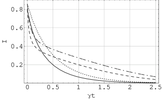
Figure 12: Time evolution of the mutual information of Gaussian states in an environment with $\gamma_{1}=\gamma_{2}=\gamma$ and $\mu_{1}=\mu_{2}=1/3$. The continuous line refers to an entangled state with $a=2$, $b=c_{1}=-c_{2}=1$ in a non squeezed environment; the dotted line refers to the same state in an environment with $r_{1}=r_{2}=1$; the dashed line refers to a non entangled state with $a=b=2$, $c_{1}=-c_{2}=1.5$ in a non squeezed environment; the dot–dashed line refers to the same state in a squeezed environment with $r_{1}=r_{2}=1$. The squeezing angle $\varphi_{2}$ has always been set to $0$.

The instance of a standard form state in a tensor product of two thermal channels (parametrized by $\gamma_{i}$ and $\mu_{i\infty}$, for $i=1,2$) is especially relevant, since it gives a basic description of dissipation in most experimental settings, like fiber–mediated communication protocols. A simple analysis straightforwardly shows that in this instance both the purity and the logarithmic negativity (that is, the entanglement) of the evolving state are increasing functions of the asymptotic purities and decreasing functions of the couplings to the baths. This should be expected, recalling the well understood synergy between entanglement and purity for general quantum states: the ideal vacuum environment, whose decoherent action is entirely due to losses, is the one which better preserve both the global information of a state and its correlations.

As we have seen, two–mode squeezed thermal states constitute a relevant class of Gaussian states, parametrized by their purity $\mu$ and by the squeezing parameter $r$ according to Eqs. (59). In particular, two–mode squeezed vacuum states (or twin-beams), which can be defined as squeezed thermal states with $\mu=1$, correspond to maximally entangled symmetric states for fixed marginal purities [17]. Therefore, they constitute a crucial resource for quantum information processing in the continuous variable scenario. For squeezed thermal states (chosen as initial conditions in the channel), it can be shown analytically that the partially transposed symplectic eigenvalue $\tilde{\nu}_{-}$ is at any time an increasing function of the bath squeezing angle $\varphi_{2}$: “parallel” squeezing in the two channels optimizes the preservation of entanglement. Both in the instance of two equal squeezed baths (i.e. with $r_{1}=r_{2}=r$) and of a thermal bath joined to a squeezed one (i.e. $r_{1}=r$ and $r_{2}=0$), it can be shown that $\tilde{\nu}_{-}$ is an increasing function of $r$ [80]. Such analytical considerations, supported by a broader numerical analysis, clearly show that a local squeezing of the environment faster degrades the entanglement of the initial state. The same behavior occurs for purity.

In order to illustrate the behaviour of the nonclassical depth $\tau$ in the noisy channel, let us consider standard form states evolving in thermal environments. For simplicity, let us assume $\gamma_{1}=\gamma_{2}=\gamma$. According to Eqs. (16) and (65), one has, for the evolving nonclassicality (recalling that $|c_{2}|\geq|c_{1}|$)

$$\begin{split}\tau(t)=&\frac{1}{2}-\frac{1}{2}(a+b)\,{\rm e}^{-\gamma t}-\frac{\mu_{1\infty}+\mu_{2\infty}}{4\mu_{1\infty}\mu_{2\infty}}(1-\,{\rm e}^{-\gamma t})\\ &+\frac{1}{2}\sqrt{\left((a-b)\,{\rm e}^{-\gamma t}+\frac{\mu_{1\infty}-\mu_{2\infty}}{2\mu_{1\infty}\mu_{2\infty}}(1-\,{\rm e}^{-\gamma t})\right)^{2}+4c_{2}^{2}\,{\rm e}^{-2\gamma t}}\Bigg{)}\,.\end{split}$$ (70)

This function is a decreasing function of the parameters $\mu_{i\infty}$: the thermal noise contributes to destroy the nonclassical features of the initial state. To study the effect of the squeezing of the bath on the nonclassical depth, we specialize to the instance of two mode squeezed thermal states, which are an archetypical class of nonclassical two mode states, characterized by squeezing in combined quadratures. In this case it can be easily shown that, in order to minimize the smaller eigenvalue of $\boldsymbol{\sigma}$ (thus maximizing $\tau$) the choice $\varphi_{2}=0$ is optimal. We will thus make such a choice in the following. The nonclassical depth of the initial two mode squeezed state $\xi_{\mu,r}$ in a channel with parameters $\mu_{i\infty}$ and $r_{i\infty}$ for $i=1,2$, takes the following form

$$\begin{split}\tau(t)=&\frac{1}{2}-\frac{\cosh(2r)}{2\sqrt{\mu}}\,{\rm e}^{-\gamma t}-\frac{\,{\rm e}^{-2r_{1\infty}}\mu_{2\infty}+\,{\rm e}^{-2r_{2\infty}}\mu_{1\infty}}{4\mu_{1\infty}\mu_{2\infty}}(1-\,{\rm e}^{-\gamma t})\\ &+\frac{1}{2}\sqrt{\left(\frac{\,{\rm e}^{-2r_{1\infty}}\mu_{2\infty}-\,{\rm e}^{-2r_{2\infty}}\mu_{1\infty}}{2\mu_{1\infty}\mu_{2\infty}}(1-\,{\rm e}^{-\gamma t})\right)^{2}+\frac{\sinh(2r)^{2}}{\mu}\,{\rm e}^{-2\gamma t}}\,.\end{split}$$ (71)

Eq. (71) reduces to the following simple form for the evolution in equal baths (with $\mu_{1\infty}=\mu_{2\infty}=\sqrt{\mu}$ and $r_{1\infty}=r_{2\infty}=r_{\infty}$)

$$\tau(t)=\frac{1-\frac{{\rm e}^{-2r}}{\sqrt{\mu}}\,{\rm e}^{-\gamma t}-\frac{{\rm e}^{-2r_{\infty}}}{\sqrt{\mu_{\infty}}}\,(1-{\rm e}^{-\gamma t})}{2}\;.$$ (72)

As can be seen in Fig. 13, the local squeezing of the baths, reducing the quantum noise in one quadrature of the multimode system, drastically increases the duration of the nonclassicality of the state and, generally, the value of its nonclassical depth at any given time. This is due to the symmetry of two mode squeezed states under mode exchange: such states can take advantage of reduced fluctuations of any quadrature of the bath. Interestingly, while the nonclassical depth is enhanced by the local squeezing of a quadrature (thus implying an improved preservation of nonclassical features like subpoissonian photon number distributions), the entanglement is not. This is due to the intrinsically non local nature of the entanglement: the advantage which could be achieved by squeezing a local quadrature is balanced by the increased fluctuations in the conjugated quadrature, which usually makes squeezing not favourable to the aim of preserving entanglement.

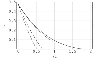
Figure 13: Evolution of the nonclassical depth of an initial two-mode squeezed thermal state with $\mu=0.9$ and $r=1.5$. The dashed line refers to the evolution in a non squeezed bath with $\mu_{1\infty}=\mu_{2\infty}=0.5$; the dot-dashed line refers to a non squeezed bath with $\mu_{1\infty}=0.25$ and $\mu_{2\infty}=1$; the dotted line refers to a bath with $\mu_{1\infty}=\mu_{2\infty}=0.5$ and $r_{1}=r_{2}=0.2$; finally, the continuous line refers to a bath with $\mu_{1\infty}=\mu_{2\infty}=0.5$, $r_{1\infty=0.6}$ and $r_{2\infty}=0$.

8 Concluding remarks

We have carried out a quantitative analysis of decoherence of continuous variable systems interacting with general Gaussian environments and reviewed many related results. The method we have presented to study the decoherence rate may be applied to other systems of interest, like qubit systems under non unitary evolutions. Several relevant configurations have been considered and exhaustively analysed, characterizing their rate of decoherence by keeping track of the decay of the global degree of purity, of indicators of nonclassicality and, for two mode states, of quantum and total correlations.

Quite in general, we have shown that, as long as one restricts to the Gaussian setting, squeezing the bath (or, equivalently, the intial state while letting the bath being thermal) does not help to better preserve either the overall coherence of the state or its quantum correlations. However, such a squeezing proves effective in delaying the decoherence of more deeply non classical states, like cat-like states resulting from coherent superpositions of Gaussian states or of number states. Furthermore, quite interestingly, we have shown that a local squeezing of the baths may improve the preservation of the mutual information in two-mode systems.

We remark that our results are of direct interest to recent developments in experimental quantum optics, especially related to quantum information and quantum control. Indeed, a crucial step towards the development of quantum information technology is the achievement of a sufficent quantum control capability, i.e. of the ability of engineering quantum signals and feedback techniques acting on the dynamics of a quantum system. In fact, the implementation of any quantum information protocol relies on maintaining quantum coherence in the system for a significant period of time and so requires some kind of mechanism to eliminate or mitigate the undesirable effects of decoherence. In this framework, a precise knowledge of the decoherence dynamics is desirable, especially in the continuous variable regime, where the field of quantum control originated and has a strong experimental impact [82, 83].

In order to make this point clearer, let us explicitly regard the following example. Consider the continuous variable teleportation of a single-mode coherent state by exploiting a two-mode squeezed thermal state as entangled resource (for a detailed description of the protocol, see Ref. [84]). Now, it may be shown [85] that the optimal teleportation fidelity $F$ (averaged over the whole complex plane) for such a protocol is given by a simple function of the smallest partially transposed symplectic eigenvalue $\tilde{\nu}_{-}$ of the two–mode squeezed state:

$$F=\frac{1}{1+2\tilde{\nu}_{-}}\;.$$ (73)

If the two modes which share the entangled state are, say, stored in two distant cavities, waiting to be used, the decoherence they experience will gradually corrupt the fidelity of the teleportation protocol. Our study allows to keep track of the quantity $\tilde{\nu}_{-}$ during the dissipative evolution of the state as a function of various environmental parameters, and thus to exactly determine the teleportation fidelity achievable as a function of time. For instance, considering an initially pure shared two-mode squeezed vacuum with squeezing parameter $r$, evolving in two environments with, for simplicity, the same coupling $\gamma$ and asymptotic purity $\mu_{\infty}$, one gets

$$F(t)=\frac{1}{1+\,{\rm e}^{-2r-\gamma t}+(1-\,{\rm e}^{-\gamma t})/\mu_{\infty}}\,.$$ (74)

Notice that such a result takes into account both losses and thermal noise. In the more general instance, let us remark that the entanglement time, extensively analyzed in Sec. 7 [see Eqs. (67-69)] and which may be analytically determined following the approach we have presented, coincides with the time over which quantum teleportation allows to beat the classical fidelity, equal to $0.5$, as shown by Eq. (73) (at $t_{ent}$ $\tilde{\nu}_{-}$ reaches 1/2 and then keeps increasing). After such a time the entanglement is gone because of local decoherence: the shared resource becomes useless to quantum informational aims.

Appendix A Determination of mixedness and entanglement of two-mode states

Here we provide explicit expressions which allow to determine the exact evolution in uncorrelated channels with $\gamma_{1}=\gamma_{2}=\gamma$ of a generic initial state in standard form. The relevant quantities $E_{{\cal N}}$, $\mu$, $S_{V}$, $I$ and $\tau$ are all functions of the four $Sp_{(2,\mathbb{R})}\oplus Sp_{(2,\mathbb{R})}$ invariants $\,{\rm Det}\,\boldsymbol{\alpha}$, $\,{\rm Det}\,\boldsymbol{\beta}$ $\,{\rm Det}\,\boldsymbol{\gamma}$ and $\,{\rm Det}\,\boldsymbol{\sigma}$. Let us then write these quantities as follows

$${\rm Det}\,\boldsymbol{\sigma} = \sum_{k=0}^{4}\Sigma_{k}\,{\rm e}^{-k\Gamma t}\;,$$ (75)

$${\rm Det}\,\boldsymbol{\alpha} = \sum_{k=0}^{2}\alpha_{k}\,{\rm e}^{-k\Gamma t}\;,$$ (76)

$${\rm Det}\,\boldsymbol{\beta} = \sum_{k=0}^{2}\beta_{k}\,{\rm e}^{-k\Gamma t}\;,$$ (77)

$${\rm Det}\,\boldsymbol{\gamma} = \gamma_{2}\,{\rm e}^{-2\Gamma t}\;,$$ (78)

defining the sets of coefficients $\Sigma_{i}$, $\alpha_{i}$, $\beta_{i}$, $\gamma_{i}$. One has

$$\Sigma_{4}= a^{2}b^{2}+\frac{a^{2}}{4\mu^{2}_{2}}+\frac{b^{2}}{4\mu^{2}_{1}}-a^{2}b\frac{\cosh 2r_{2}}{\mu_{2}}-ab^{2}\frac{\cosh 2r_{1}}{\mu_{1}}+ab\frac{\cosh 2r_{1}\cosh 2r_{2}}{\mu_{1}\mu_{2}}-a\frac{\cosh 2r_{1}}{4\mu_{1}\mu_{2}^{2}}-b\frac{\cosh 2r_{2}}{4\mu_{1}^{2}\mu_{2}}$$ (79)

$$+(c_{1}^{2}+c_{2}^{2})\left(a\frac{\cosh 2r_{2}}{2\mu_{2}}+\frac{b\cosh 2r_{1}}{2\mu_{1}}-\frac{\cosh 2r_{1}\cosh 2r_{2}}{4\mu_{1}\mu_{2}}-\frac{\sinh 2r_{1}\sinh 2r_{2}\cos 2\varphi_{2}}{4\mu_{1}\mu_{2}}-ab\right)$$

$$+(c_{1}^{2}-c_{2}^{2})\left(a\frac{\sinh 2r_{2}\cos 2\varphi_{2}}{2\mu_{2}}+b\frac{\sinh 2r_{1}}{2\mu_{1}}-\frac{\sinh 2r_{1}\cosh 2r_{2}}{4\mu_{1}\mu_{2}}-\frac{\cosh 2r_{1}\sinh 2r_{2}\cos 2\varphi_{2}}{4\mu_{1}\mu_{2}}\right)$$

$$+c_{1}^{2}c_{2}^{2}+\frac{1}{16\mu_{1}^{2}\mu_{2}^{2}}\;,$$

$$\Sigma_{3}= -2\frac{a^{2}}{4\mu^{2}_{2}}-2\frac{b^{2}}{4\mu^{2}_{1}}+a^{2}b\frac{\cosh 2r_{2}}{\mu_{2}}+ab^{2}\frac{\cosh 2r_{1}}{\mu_{1}}-2ab\frac{\cosh 2r_{1}\cosh 2r_{2}}{\mu_{1}\mu_{2}}+3a\frac{\cosh 2r_{1}}{4\mu_{1}\mu_{2}^{2}}+3b\frac{\cosh 2r_{2}}{4\mu_{1}^{2}\mu_{2}}$$ (80)

$$-(c_{1}^{2}-c_{2}^{2})\left(a\frac{\sinh 2r_{2}\cos 2\varphi_{2}}{2\mu_{2}}+b\frac{\sinh 2r_{1}}{2\mu_{1}}-2\frac{\sinh 2r_{1}\cosh 2r_{2}}{4\mu_{1}\mu_{2}}-2\frac{\cosh 2r_{1}\sinh 2r_{2}\cos 2\varphi_{2}}{4\mu_{1}\mu_{2}}\right)$$

$$-(c_{1}^{2}+c_{2}^{2})\left(a\frac{\cosh 2r_{2}}{2\mu_{2}}+\frac{b\cosh 2r_{1}}{2\mu_{1}}-2\frac{\cosh 2r_{1}\cosh 2r_{2}}{4\mu_{1}\mu_{2}}-2\frac{\sinh 2r_{1}\sinh 2r_{2}\cos 2\varphi_{2}}{4\mu_{1}\mu_{2}}\right)$$

$$-\frac{1}{4\mu_{1}^{2}\mu_{2}^{2}}\,,$$

$$\Sigma_{2}= \frac{a^{2}}{4\mu^{2}_{2}}+\frac{b^{2}}{4\mu^{2}_{1}}+ab\frac{\cosh 2r_{1}\cosh 2r_{2}}{\mu_{1}\mu_{2}}-3a\frac{\cosh 2r_{1}}{4\mu_{1}\mu_{2}^{2}}-3b\frac{\cosh 2r_{2}}{4\mu_{1}^{2}\mu_{2}}$$ (81)

$$-(c_{1}^{2}+c_{2}^{2})\left(\frac{\cosh 2r_{1}\cosh 2r_{2}}{4\mu_{1}\mu_{2}}+\frac{\sinh 2r_{1}\sinh 2r_{2}\cos 2\varphi_{2}}{4\mu_{1}\mu_{2}}\right)$$

$$-(c_{1}^{2}-c_{2}^{2})\left(\frac{\sinh 2r_{1}\cosh 2r_{2}}{4\mu_{1}\mu_{2}}+\frac{\cosh 2r_{1}\sinh 2r_{2}\cos 2\varphi_{2}}{4\mu_{1}\mu_{2}}\right)+\frac{1}{16\mu_{1}^{2}\mu_{2}^{2}}\;,$$

$$\Sigma_{1}=+a\frac{\cosh 2r_{1}}{4\mu_{1}\mu_{2}^{2}}+b\frac{\cosh 2r_{2}}{4\mu_{1}^{2}\mu_{2}}-\frac{1}{4\mu_{1}^{2}\mu_{2}^{2}}\;,$$ (82)

$$\Sigma_{0}=\frac{1}{16\mu_{1}^{2}\mu_{2}^{2}}\;,$$ (83)

$$\alpha_{2} = a^{2}-a\frac{\cosh 2r_{1}}{\mu_{1}}+\frac{1}{4\mu_{1}^{2}}\;,$$ (84)

$$\alpha_{1} = a\frac{\cosh 2r_{1}}{\mu_{1}}-2\frac{1}{4\mu_{1}^{2}}\;,$$ (85)

$$\alpha_{0} = \frac{1}{4\mu_{1}^{2}}\;,$$ (86)

$$\beta_{2} = b^{2}-b\frac{\cosh 2r_{2}}{\mu_{2}}+\frac{1}{4\mu_{2}^{2}}\;,$$ (87)

$$\beta_{1} = b\frac{\cosh 2r_{2}}{\mu_{2}}-2\frac{1}{4\mu_{2}^{2}}\;,$$ (88)

$$\beta_{0} = \frac{1}{4\mu_{2}^{2}}\;,$$ (89)

$$\gamma_{2} = c_{1}c_{2}\;.$$ (90)

The coefficients of Eq. (66), whose solution $k_{ent}$ allows to determine the entanglement time of an arbitrary two–mode Gaussian state, read

$$u = \Sigma_{4}\;,$$ (91)

$$v = \Sigma_{3}\;,$$ (92)

$$w = \Sigma_{2}-\alpha_{2}-\beta_{2}-|\gamma_{2}|\;,$$ (93)

$$y = \Sigma_{1}-\alpha_{1}-\beta_{1}\;,$$ (94)

$$z = \Sigma_{0}-\alpha_{0}-\beta_{0}+\frac{1}{4}\;.$$ (95)

References

- [1] Quantum Information Theory with Continuous Variables, S. L. Braunstein and A. K. Pati Eds. (Kluwer, Dordrecht, 2002), and references therein.
- [2] S. L. Braunstein and P. van Loock, quant-ph/0410100; Rev. Mod. Phys., to be published.
- [3] A. Furusawa, J. L. Sorensen, S. L. Braunstein, C. A. Fuchs, H. J. Kimble, and E. S. Polzik, Science 282, 706 (1998); T. C. Zhang, K. W. Goh, C. W. Chou, P. Lodahl, and H. J. Kimble, Phys. Rev. A 67, 033802 (2003).
- [4] F. Grosshans and P. Grangier, Phys. Rev. Lett. 88, 057902 (2002); F. Grosshans, G. Van Assche, J. Wenger, R. Brouri, N. J. Cerf, and P. Grangier, Nature 421, 238 (2003).
- [5] A. O. Caldeira and A. J. Leggett, Physica A 121, 587 (1983).
- [6] W. H. Zurek, Physics Today 44 (10), 36 (1991).
- [7] S. M. Barnett and P. M. Radmore, Methods in Theoretical Quantum Optics (Clarendon Press, Oxford, 1997).
- [8] C. T. Lee, Phys. Rev. A 44, R2275 (1991).
- [9] M. S. Kim, W. Son, V. Buzek, and P. L. Knight, Phys. Rev. A 65, 032323 (2002).
- [10] M. Takeoka, M. Ban, and M. Sasaki, J. Opt. B: Quantum Semiclass. Opt. 4, 114 (2002).
- [11] M. G. Benedict and A. Czirják, Phys. Rev. A 60, 4034 (1999); A. Kenfack and K. Życzkowski, J. Opt. B: Quantum Semiclass. Opt.6, 396 (2004).
- [12] R. Simon, E. C. G. Sudarshan, and N. Mukunda, Phys. Rev. A 36, 3868 (1987).
- [13] Arvind, B. Dutta, N. Mukunda, and R. Simon, Pramana 45, 471 (1995); quant-ph/9509002.
- [14] J. Williamson, Am. J. Math. 58, 141 (1936); see also V.I. Arnold, Mathematical Methods of Classical Mechanics, (Springer-Verlag, New York, 1978) and R. Simon, S. Chaturvedi, and V. Srinivasan., J. Math. Phys. 40, 3632 (1999).
- [15] R. Simon, N. Mukunda, and B. Dutta, Phys. Rev. A 49, 1567 (1994).
- [16] G. Adesso, A. Serafini, and F. Illuminati, Phys. Rev. Lett. 92, 087901 (2004).
- [17] G. Adesso, A. Serafini, and F. Illuminati, Phys. Rev. A 70, 022318 (2004).
- [18] G. Adesso, A. Serafini, and F. Illuminati, Phys. Rev. Lett. 93, 220504 (2004).
- [19] A. Serafini, G. Adesso, and F. Illuminati, quant-ph/0411109, and Phys. Rev. A 71 (2005), in press.
- [20] G. Adesso and F. Illuminati, quant-ph/0410050.
- [21] A. K. Ekert, C. Moura Alves, and D. K. L. Oi, Phys. Rev. Lett. 88, 217901 (2002); R. Filip, Phys. Rev. A 65, 062320 (2002).
- [22] J. Fiurášek and N. J. Cerf, Phys. Rev. Lett. 93, 063601 (2004); J. Wenger, J. Fiurášek, R. Tualle-Brouri, N. J. Cerf, and Ph. Grangier, Phys. Rev. A 70, 053812 (2004).
- [23] A. S. Holevo, M. Sohma, and O. Hirota, Phys. Rev. A 59, 1820 (1999).
- [24] A. Serafini, F. Illuminati, and S. De Siena, J. Phys. B: At. Mol. Op. Phys. 37, L21 (2004).
- [25] L. Henderson and V. Vedral, J. Phys. A: Math. Gen. 34, 6899 (2001).
- [26] R. Simon, Phys. Rev. Lett. 84, 2726 (2000).
- [27] L.-M. Duan, G. Giedke, J. I. Cirac, and P. Zoller, Phys. Rev. Lett. 84, 2722 (2000).
- [28] G. Vidal and R. F. Werner, Phys. Rev. A 65, 032314 (2002).
- [29] J. Eisert, PhD thesis, University of Potsdam (Potsdam, 2001).
- [30] K. Audenaert, M. B. Plenio, and J. Eisert, Phys. Rev. Lett. 90, 027901 (2003).
- [31] D. Walls and G. Milburn, Quantum optics (Springer Verlag, Berlin, 1994).
- [32] Possible squeezed reservoirs are treated in M.-A. Dupertuis and S. Stenholm, J. Opt. Soc. Am. B 4, 1094 (1987); M.-A. Dupertuis, S. M. Barnett, and S. Stenholm, ibid. 4, 1102 (1987); Z. Ficek and P. D. Drummond, Phys. Rev. A 43, 6247 (1991); K. S. Grewal, Phys Rev A 67, 022107 (2003); see also C. W. Gardiner and P. Zoller, Quantum Noise (Springer Verlag, Berlin, 1999), M. S. Kim and N. Imoto, Phys. Rev. A 52, 2401 (1995) and Ref. [31].
- [33] P. Tombesi and D. Vitali, Phys. Rev. A 50, 4253 (1994); P. Tombesi, and D. Vitali, Appl. Phys. B 60, S69 (1995).
- [34] J. F. Poyatos, J. I. Cirac, and P. Zoller, Phys. Rev. Lett. 77, 4728 (1996); N. Lütkenhaus, J. I. Cirac, and P. Zoller, Phys. Rev. A 57, 548 (1998).
- [35] H. M. Wiseman and G. J. Milburn, Phys. Rev. Lett. 70, 548 (1993); H. M. Wiseman and G. J. Milburn, Phys. Rev. A 49, 1350 (1994).
- [36] M. G. A. Paris, F. Illuminati, A. Serafini, and S. De Siena, Phys. Rev. A 68, 012314 (2003).
- [37] J.I. Cirac, J. Eisert, G. Giedke, M. Lewenstein, M.B. Plenio, R.F. Werner, and M.M. Wolf, textbook in preparation (2004).
- [38] A. Serafini, J. Eisert, and M. M. Wolf, Phys. Rev. A 71, 012320 (2005).
- [39] O. Brodier and A. M. Ozorio de Almeida, Phys. Rev. E 69, 016204 (2004).
- [40] P. Marian and T. A. Marian, Phys. Rev. A 47, 4487 (1993).
- [41] R. W. Rendell and A. K. Rajagopal, Phys. Lett. A 279, 175 (2001).
- [42] V. Giovannetti, S. Guha, S. Lloyd, L. Maccone, and J. H. Shapiro, Phys. Rev. A 70, 032315 (2004); V. Giovannetti, S. Lloyd, L. Maccone, J. H. Shapiro, and B. J. Yen, Phys. Rev. A 70, 022328 (2004).
- [43] W. H. Zurek, S. Habib, and J. P. Paz, Phys. Rev. Lett. 70, 1187 (1993).
- [44] A. Venugopalan, Phys. Rev. A 61, 012102 (1999).
- [45] E. Schrödinger, Naturwissenschaften 23, 812 (1935).
- [46] B. Yurke and D. Stoler, Phys. Rev. Lett. 57, 13 (1986).
- [47] A. Mecozzi and P. Tombesi, Phys. Rev. Lett. 58, 1055 (1987); B. Yurke, W. Schleich, and D. F. Walls, Phys. Rev. A 42, 1703 (1990); T. Ogawa, M Ueda, N. Imoto, Phys. Rev. A 43, 6458 (1991); M. Brune, S. Haroche, J. M. Raimond, L. Davidovich, and N. Zagury, Phys. Rev. A 45, 5193 (1992); M. Dakna, T. Anhut, T. Opatrny, L. Knöll, and D. G. Welsch, Phys. Rev. A 55, 3184 (1997); S. Olivares, M. G. A. Paris and A. R. Rossi, Phys. Lett. A 319, 32 (2003); A. R. Rossi, S. Olivares, and M. G. A. Paris, J. Mod. Opt. 51, 1057 (2004); M. Paternostro, M. S. Kim, and B. S. Ham, Phys. Rev. A 67, 023811 (2003); see also V. V. Dodonov, J. Opt. B: Quantum Semiclass. Opt. 4, R1 (2002) and references therein.
- [48] M. Brune, E. Hagley, J. Dreyer, X. Maître, A. Maali, C. Wunderlich, J.M. Raimond, and S. Haroche, Phys. Rev. Lett. 77, 4887 (1996); A. Auffeves, P. Maioli, T. Meunier, S. Gleyzes, G. Nogues, M. Brune, J. M. Raimond, and S. Haroche, Phys. Rev. Lett. 91, 230405 (2003).
- [49] C. Monroe, D. M. Meekhof, B. E. King, and D. J. Wineland, Science 272, 1131 (1996).
- [50] C. J. Myatt, B. E. King, Q. A. Turchette, C. A. Sackett, D. Kielpinski, W. M. Itano, C. Monroe, and D. J. Wineland, Nature 403, 269 (2000).
- [51] D. F. Walls, G. J. Milburn, Phys. Rev. A 31, 2403 (1985).
- [52] T. A. B. Kennedy and D. F. Walls, Phys. Rev. A 37, 152 (1988).
- [53] P. Goetsch, P. Tombesi, and D. Vitali, Phys. Rev. A 54, 4519 (1996); S. Zippilli, D. Vitali, P. Tombesi, and J.-M. Raimond, ibid. 67, 052101 (2003).
- [54] F. A. A. El-Orany, Phys. Rev. A 65, 043814 (2002).
- [55] A. Serafini, S. De Siena, F. Illuminati, and M. G. A. Paris, J. Opt. B: Quantum and Semiclass. Opt. 6, S591 (2004).
- [56] B. M. Garraway, P. L. Knight, and M. B. Plenio, Phys. Scr. T76, 152 (1998).
- [57] H.-K. Lo and H. F. Chau, Science 283, 2050 (1999); H. Zbinden, N. Gisin, B. Huttner, and W. Tittel, J. Cryptol. 13, 207 (2000); T. Jennewein, C. Simon, G. Weihs, H. Weinfurter, and A. Zeilinger, Phys. Rev. Lett. 84, 4729 (2000).
- [58] K. M. Gheri, C. Saavedra, P. Törmä, J. I. Cirac, and P. Zoller, Phys. Rev. A 58, R2627 (1998); S. J. van Enk, J. I. Cirac, and P. Zoller, Science 279, 205 (1998).
- [59] S. Y. Kilin and D. B. Horosko, Phys. Rev. Lett. 74, 5206 (1995); W. Leonski, S. Dyrting, and R. Tanas, J. Mod. Opt. 44, 2105 (1997); A. Vidiella-Barranco, and J. A. Roversi, Phys. Rev. A 58 , 3349 (1998); W. Leonski, Phys. Rev. A 54, 3369 (1969).
- [60] M. G. A. Paris, Int. J. Mod. Phys. B 11, 1913 (1997); M. Dakna, T. Anhut, T. Opatrny, L. Knoll, and D. G. Welsch, Phys. Rev. A 55, 3184 (1997); O. Steuernagel, Opt Comm 138 71 (1997).
- [61] G. M. D’Ariano, L. Maccone, M. G. A. Paris, M. F. Sacchi, Phys. Rev. A 61 053817 (2000); Fort. Phys. 48, 511 (2000).
- [62] K. Vogel, V. M. Akulin, and W. P. Scheich, Phys. Rev. Lett. 71, 1816 (1993).
- [63] C. J. Villas-Bôas, F. R. de Paula, R. M. Serra, and M. H. Y. Moussa, Phys. Rev. A 68, 053808 (2003).
- [64] B. T. H. Varcoe, S. Brattke, M. Weidinger, and H. Walther, Nature 403, 743 (2000); S. Brattke, B. T. H. Varcoe, and H. Walther, Phys. Rev. Lett. 86 3534 (2001).
- [65] K. R. Brown, K. M. Dani, D. M. Stamper-Kurn, and K. B. Whaley, Phys. Rev. A 67, 043818 (2003).
- [66] G. Harel and G. Kurizki, Phys. Rev. A 54, 5410 (1996); G. Harel, G. Kurizki, J. K. McIver, and E. Coutsias, Phys. Rev. A 53, 4534 (1996).
- [67] D. M. Meekhof, C. Monroe, B. E. King, W. M. Itano, and D. J. Wineland, Phys. Rev. Lett. 76, 1796 (1996).
- [68] N. Nayak, quant-ph/0308077.
- [69] A. Serafini, S. De Siena, and F. Illuminati, Mod. Phys. Lett. B 18, 687 (2004).
- [70] I. Gradstein and I. Ryshik, Summen-, Produkt- und Integral- Tafeln, (Harri Deutsch Verlag, Thun Frankfurt/M, 1981).
- [71] J. Janszky, M. G. Kim, and M. S. Kim, Phys. Rev. A 53, 502 (1996).
- [72] S. Haroche, Introduction to quantum optics and decoherence, lectures held at Les Houches Summer School Quantum entanglement and information processing (2003).
- [73] L.-M. Duan and G.-C. Guo, Quantum Semiclass. Opt. 9, 953 (1997).
- [74] A. K. Rajagopal and R. W. Rendell, Phys. Rev. A 63, 022116 (2001).
- [75] T. Hiroshima, Phys. Rev. A 63, 022305 (2001).
- [76] S. Scheel and D.-G. Welsch, Phys. Rev. A 64, 063811 (2001).
- [77] M. G. A Paris Entangled light and applications in Trends in Quantum Physics, V. Krasnoholovets and F. Columbis Eds., p. 89 (Nova Publisher, Hauppauge NY, 2004).
- [78] D. Wilson, J. Lee, and M. S. Kim, J. Mod. Opt. 50, 1809 (2003).
- [79] J. S. Prauzner–Bechcicki, J. Phys. A: Math. Gen. 37, L173 (2004).
- [80] A. Serafini, F. Illuminati, M. G. A. Paris, and S. De Siena, Phys. Rev. A 69, 022318 (2004).
- [81] S. M. Barnett, S. J. D. Phoenix, Phys. Rev. A 40, 2404 (1989); S. M. Barnett, S. J. D. Phoenix, ibid. 44, 535 (1991); M. G. A. Paris, ibid. 59, 1615 (1999).
- [82] C. E. Wieman, D. E. Pritchard, and D. J. Wineland Rev. Mod. Phys. 71, S253-S262 (1999).
- [83] L. M. K. Vandersypen and I. L. Chuang Rev. Mod. Phys. 76, 1037 (2004).
- [84] S. L. Braunstein and H. J. Kimble, Phys. Rev. Lett. 80, 869 (1998).
- [85] G. Adesso and F. Illuminati, quant-ph/0412125.