Heuristic explanation of quantum interference experiments

Abstract

A particle is described as a non-spreading wave packet satisfying a linear equation within the framework of special relativity. Young’s and other interference experiments are explained with a hypothesis that there is a coupling interaction between the peaked and non-peaked pieces of the wave packet. This explanation of the interference experiments provides a realistic interpretation of quantum mechanics. The interpretation implies that there is physical reality of particles and no wave function collapse. It also implies that neither classical mechanics nor current quantum mechanics is a complete theory for describing physical reality and the Bell inequalities are not the proper touchstones for reality and locality. The problems of the boundary between the macro-world and micro-world and the de-coherence in the transition region (meso-world) between the two are discussed. The present interpretation of quantum mechanics is consistent with the physical aspects of the Copenhagen interpretation, such as, the superposition principle, Heisenberg’s uncertainty principle and Born’s probability interpretation, but does not favor its philosophical aspects, such as, non-reality, non-objectivity, non-causality and the complementary principle.

Key words: quantum interference, wave-particle duality, non-spreading wave packet
PACS: 03.65.-w

1 Introduction

In 1801 Thomas Young performed a two-pinhole light interference experiment and demonstrated light to have a wave nature against the tide of favor for Newton’s corpuscular theory of light at that times [1]. Almost a century after, taking Planck’s quantum hypothesis [2] a big step further, Albert Einstein proposed that light is made up of particles and successfully explained the photoelectric effect [3]. His explanation of the effect suggests that light has wave-particle duality, the central problem of quantum physics. Later, on the basis of Planck and Einstein’s quantum theories, Louis de Broglie proposed that perhaps matter also has wave properties [4]. His matter wave hypothesis was confirmed by Davisson and Germer’s electron diffraction experiment [5]. In addition, in the last century there were two experiments first demonstrating diffraction and interference of single particles and illustrating the wave-particle duality: a needle diffraction experiment with single photons reported in 1909 by Taylor [6] and an interference experiment with single electrons by using an electron bi-prism reported in 1989 by Tonomura and co-workers [7]. However, in the past almost hundred years physicists and others were unable to find a convincing way to solve the wave-particle duality problem. It still remains a baffling and fascinating mystery to us today. As the paradigm experiment of quantum mechanics, Young’s experiment with single photons is mentioned in more or less details in quantum textbooks. We learn in them that if the intensity of a beam of single-frequency light is lowered so much that photons pass one after the other through two slits at a barrier, after a long time exposure an interference pattern consisting of tiny discrete spots emerges on a detector screen some distance behind the barrier. It implies that the photon is somehow divided into two pieces passing through both slits simultaneously and interfering with each other. For the path problem of particles, Heisenberg said: $``$the $`$path<sup>′</sup> comes into being only because we observe it<sup>′′</sup> [8]. The Copenhagen interpretation of quantum mechanics asserts that observation creates reality. Although the assertion has been accepted readily or reluctantly by many physicists, nevertheless physicists and students still like to ask: $``$How can a particle pass through both slits simultaneously and interfere with itself?^′′ This article attempts to explain quantum interference experiments, solve the wave-particle duality problem and answer the question.

2 Description of particles

As well known, de Broglie first introduced a wave group associated with a particle that its group velocity is, in a first-order approximation, the velocity of the particle [4]. But the wave group spreads in time. Later he proposed a pilot-wave theory [9] and in the mid-fifties of the last century he considered a particle to be a soliton-like structure satisfying a non-linear differential equation [10]. Nevertheless he also did not succeed much in this direction. Perhaps we need to find a way out. Now, as an exploration of ways, a particle as a wave-particle entity is described in the following by means of a non-spreading wave packet satisfying a linear equation within the framework of special relativity.

We recall that de Broglie’s original theory of matter waves in his doctoral thesis is essentially relativistic [4]. To gain insight into the quantum world we still need to resort to the special theory of relativity. Equivalently to Minkowski’s formulation of special relativity, we consider a four-dimensional system $(x,y,x,w)$ and assume that a particle moves at the light speed $c$ in accordance with the following equation:

$$c^{2}t^{2}=x_{0}^{2}+y_{0}^{2}+z_{0}^{2}+w_{0}^{2},\mbox{ }w_{0}=c\tau_{0}$$ (1)

where $\tau_{0}$ is the proper time. The variable $w$ is much like the spatial ones, $x$, $y$ and $z$. From Eq.(1) we can draw a figure (Fig.1) to show the motion of the particle and illustrate Einstein’s mass-velocity relation.

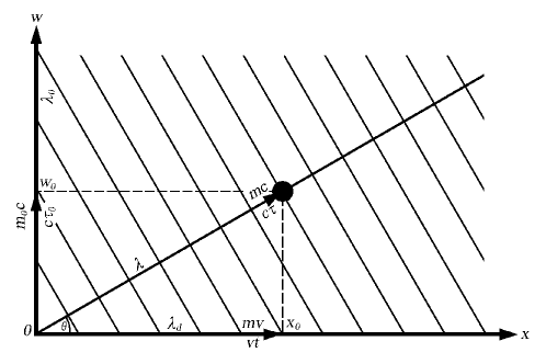
Figure 1: Illustration of Einstein’s mass-velocity relation and graphic display of the Compton wavelength $\lambda_{0}$, transformed Compton wavelength $\lambda$ and relativistic de Broglie wavelength $\lambda_{d}$.

In this figure only the two-dimensional system $(x,w)$ is drawn for the purpose of this article and $x_{0}=vt$ is given. Assuming that the quantities $m_{0}c$ and $mv$ are the components of $``$momentum^′′ $mc$ in the $w$ and $x$ directions where $m$ is the mass of the particle, from this figure we can write the following relations:

$$m=\frac{m_{0}}{\sqrt{1-v^{2}/c^{2}}}$$ (2)

$$mc^{2}=m_{0}c^{2}\sqrt{1-v^{2}/c^{2}}+mv^{2}$$ (3)

Concerning the wave property of the particle, according to de Broglie [4], we have the Compton wavelength $\lambda_{0}$, transformed Compton wavelength $\lambda$ and relativistic de Broglie wavelength $\lambda_{d}$:

$$\lambda_{0}=2\pi\hbar/m_{0}c$$ (4)

$$\lambda=2\pi\hbar/mc$$ (5)

$$\lambda_{d}=2\pi\hbar/mv$$ (6)

which are shown in Fig.1.

Now we assume a sharply localized wave packet composed of infinite harmonic waves propagating at the same phase speed $c$ in the four dimensions. If the center of the wave packet is at the origin of the coordinate system when $t$=$0$, as a model, it can be approximately written as the following Fourier integral associated with a four-dimensional Dirac delta function:

$$B(\textbf{R},t)=\frac{N}{(2\pi)^{4}}\int{e^{-i(2\pi vt-\textbf{\scriptsize{K}}\cdot\textbf{\scriptsize{R}})}}\mbox{d}K_{x}\mbox{d}K_{y}\mbox{d}K_{z}\mbox{d}K_{w},\mbox{ }\left|\textbf{K}\right|=K=2\pi\nu/c$$ (7)

where R=$(x,y,z,w)$ is a four-dimensional position vector, K=$(K_{x},K_{y},K_{z},K_{w})$ is a four-dimensional wave vector and the wave vectors of all the constituent waves are assumed in the same direction. Since $K=2\pi\nu/c$ has been assumed, this wave packet satisfies the following linear equation:

$$\frac{\partial^{2}B}{c^{2}\partial t^{2}}-\frac{\partial^{2}B}{\partial x^{2}}-\frac{\partial^{2}B}{\partial y^{2}}-\frac{\partial^{2}B}{\partial z^{2}}-\frac{\partial^{2}B}{\partial w^{2}}=0$$ (8)

Its linearity is in accordance with the linearity of quantum mechanics, which is essential for the linear superposition principle of wave.

In order to use the wave packet to describe the particle and make it being non-spreading, we merely ascribe relativistic energy $E=mc^{2}$ and $``$momentum^′′ $P=mc$ of the particle to one component of the wave packet, called as a characteristic component. This way to avoid the indeterminacy in momentum and energy of a wave packet was proposed by H. R. Brown and R. de A. Martins [11] and G. Wang [12]. Thus, following Planck, Einstein and de Broglie’s quantum theories, assuming that $E=h\nu_{c}$ and $P=\hbar K_{c}$, we write $K$ and $\nu$ as

$$K=K_{c}+K^{\prime}=\frac{mc}{\hbar}+K^{\prime}$$ (9)

$$\nu=\nu_{c}+\nu^{\prime}=\frac{mc^{2}}{h}+\frac{cK^{\prime}}{2\pi}$$ (10)

Using Eq.(9), Eq.(10) and Eq.(3), from Eq.(7) we write the following non-spreading wave packet describing the particle:

$$B(\textbf{R},t) = \frac{N}{(2\pi)^{4}}e^{-i(2\pi\nu_{c}t-\textbf{\scriptsize{K}}_{c}\cdot\textbf{\scriptsize{R}})}\int e^{-i(2\pi\nu^{\prime}t-\textbf{\scriptsize{K}}^{\prime}\cdot\textbf{\scriptsize{R}})}\mbox{d}{K}^{\prime}_{x}\mbox{d}{K}^{\prime}_{y}\mbox{d}{K}^{\prime}_{z}\mbox{d}{K}^{\prime}_{w}$$ (11)

$$= \frac{N}{(2\pi)^{4}}e^{-i[(m_{0}c^{2}\sqrt{1-v^{2}/c^{2}}+mv^{2})t/\hbar-\textbf{\scriptsize{K}}_{c}\cdot\textbf{\scriptsize{R}}]}$$

$$\cdot\int{e^{-i(2\pi\nu^{\prime}t-\textbf{\scriptsize{K}}^{\prime}\cdot\textbf{\scriptsize{R}})}}\mbox{d}{K}^{\prime}_{x}\mbox{d}{K}^{\prime}_{y}\mbox{d}{K}^{\prime}_{z}\mbox{d}{K}^{\prime}_{w}$$

where $\textbf{K}_{c}$ is the wave vector of its characteristic component. The transformed Compton wavelength $\lambda$ equals to $2\pi/K_{c}$.

If, for simplicity of treatment, the two-dimensional coordinate system ($x,w$) is used instead of the four-dimensional system, we have

$$\textbf{K}_{c}\cdot\textbf{R}=\frac{mc}{\hbar}(x\cos\theta+w\sin\theta)=k_{c}x+\frac{m_{0}c}{\hbar}w,$$

$$\cos\theta=v/c,\mbox{ }k_{c}=mc\cos\theta/\hbar$$ (12)

$$\textbf{K}^{\prime}\cdot\textbf{R}={K}^{\prime}_{x}x+{K}^{\prime}_{w}w,\mbox{ }{K}^{\prime}_{x}={K}^{\prime}\cos\theta,\mbox{ }{K}^{\prime}_{w}={K}^{\prime}\sin\theta$$ (13)

Using Eq.(12), Eq.(13) and $cK^{\prime}$=$c(\cos^{2}\theta+\sin^{2}\theta)K^{\prime}$=$vK^{\prime}_{x}+c(1-v^{2}/c^{2})^{1/2}K^{\prime}_{w}$, Eq.(11) can be changed into the following form:

$$B(x,w,t) = \frac{M}{(2\pi)^{2}}e^{-i[(m_{0}c^{2}\sqrt{1-v^{2}/c^{2}}+mv^{2})t-(\hbar k_{c}x+m_{0}cw)]/\hbar}$$ (14)

$$\cdot\int{e^{-i[c{K}^{\prime}t-({K}^{\prime}_{x}x+{K}^{\prime}_{w}w)]}}\mbox{d}{K}^{\prime}_{x}\mbox{d}{K}^{\prime}_{w}$$

$$= \frac{M}{(2\pi)^{2}}e^{-i(vt-x)k_{c}}\int e^{-i(vt-x){K}^{\prime}_{x}}\mbox{d}{K}^{\prime}_{x}$$

$$\cdot e^{-i(c\sqrt{1-v^{2}/c^{2}}t-w)m_{0}c/\hbar}\int e^{-i(c\sqrt{1-v^{2}/c^{2}}t-w){K}^{\prime}_{w}\mbox{d}{K}^{\prime}_{w}}$$

$$= Me^{-i(vt-x)k_{c}}\delta(vt-x)e^{-i(c\sqrt{1-v^{2}/c^{2}}t-w)m_{0}c/\hbar}$$

$$\cdot\delta(c\sqrt{1-v^{2}/c^{2}}t-w)$$

where $k_{c}=mv/\hbar=p/\hbar$ is the component of $\textbf{K}_{c}$ in the $x$ direction. From Eq.(14), it is easy to write the three-dimensional relativistic wave packet that we are really interested in as follows:

$$B(\textbf{r},t)=Ce^{-i[(vp+m_{0}c^{2}\sqrt{1-v^{2}/c^{2}})t-\textbf{\scriptsize{p}}\cdot\textbf{\scriptsize{r}}]/\hbar}\delta^{3}(\textbf{v}t-\textbf{r})=\psi_{r}(\textbf{r},t)\delta^{3}(\textbf{v}t-\textbf{r}),$$

$$\psi_{r}(\textbf{v}t-\textbf{r})=Ce^{-i[(vp+m_{0}c^{2}\sqrt{1-v^{2}/c^{2}})t-\textbf{\scriptsize{p}}\cdot\textbf{\scriptsize{r}}]/\hbar},\mbox{ }p=mv,$$

$$\delta^{3}(\textbf{v}t-\textbf{r})=\delta(v_{x}t-x)\delta(v_{y}t-y)\delta(v_{z}t-z)$$ (15)

where $\psi_{r}(\textbf{r},t)$ is the relativistic de Broglie wave function with the wavelength $\lambda_{d}=2\pi\hbar/mv$ as shown in Fig.1. It is worth noting that $m_{0}c^{2}(1-\nu^{2}/c^{2})^{1/2}$ may be considered a $v$-dependent $``$internal energy^′′ and the phase speed linked to $vp=mv^{2}$ is exactly the particle speed $v$. When $v\ll c$, taking the non-relativistic approximation to the first order in $v$/$c$ and removing the $v$-independent $\textrm{exp}(-im_{0}c^{2}t/\hbar)$, Eq.(15) can be turned into the non-relativistic wave packet as follows:

$$B(\textbf{r},t)=Ce^{-i(p^{2}t/2m_{0}-\textbf{\scriptsize{p}}\cdot\textbf{\scriptsize{r}})/\hbar}\delta^{3}(\textbf{v}t-\textbf{r})=\psi(\textbf{r},t)\delta^{3}(\textbf{v}t-\textbf{r}),$$

$$\psi(\textbf{r},t)=Ce^{-i(p^{2}t/2m_{0}-\textbf{\scriptsize{p}}\cdot\textbf{\scriptsize{r}})/\hbar}$$ (16)

here $p=m_{0}v$. The $\psi(\textbf{r},t)$, namely the de Broglie wave function, clearly does not contain information about the spatial position of the particle and only implies that the particle has a uniform probability of existing everywhere in the universe. This explains in a way Born’s probability interpretation of wave function. On the other hand, the function $\delta^{3}(\textbf{v}t-\textbf{r})$ describes the trajectory movement of the peak of the wave packet. The peak can be regarded as a point-like classical particle. In fact, a real particle has a finite small size that has been approximated here by infinitesimal width of the delta function. We are aware that classical mechanics describes its trajectory movement as well as energy and momentum that now emerge in the phase of the wave function.

If we regard the spin of the electron, since the Dirac equation describes a four-component spinor, the spinor is the characteristic component set of the wave packet describing the electron. Thus the wave packet would have quadruple components.

Now, we are going to describe a photon. Since it is $``$massless^′′, $P_{w}=(K_{w})_{c}\hbar$=0. Regardless of its polarization or spin, we can describe it as a linear non-spreading wave packet in which the characteristic component is a scalar electric wave function. Assuming $\nu$=$kc/{2\pi}$ and denoting the wave vector of the component by $\textbf{k}_{c}$, from Eq.(7), by taking an similar approach used to derive Eq.(15), we write the wave packet as

$$B(\textbf{r},t)=\frac{C}{(2\pi)^{3}}e^{-i(2\pi\nu_{c}t-\textbf{\scriptsize{k}}_{c}\cdot\textbf{\scriptsize{r}})}\int e^{-i(\textbf{\scriptsize{c}}\cdot\textbf{\scriptsize{k}}^{\prime}t-\textbf{\scriptsize{k}}^{\prime}\cdot\textbf{\scriptsize{r}})}\mbox{d}{k}^{\prime}_{x}\mbox{d}{k}^{\prime}_{y}\mbox{d}{k}^{\prime}_{z}$$

$$=Ce^{-i(2\pi\nu_{c}t-\textbf{\scriptsize{k}}_{c}\cdot\textbf{\scriptsize{r}})}\delta^{3}(\textbf{c}t-\textbf{r})=\varepsilon(\textbf{r},t)\delta^{3}(\textbf{c}t-\textbf{r}),$$

$$\varepsilon(\textbf{r},t)=Ce^{-i(2\pi\nu_{\textrm{\tiny{c}}}t-\textbf{\scriptsize{k}}_{c}\cdot\textbf{\scriptsize{r}})},\mbox{ }\left|\textbf{c}\right|=c$$ (17)

It is necessary to bear in mind that only the characteristic component $\varepsilon(\textbf{r},t)$ represents the electric field associated with the photon and is ascribed the photon energy $E$=$h\nu_{\textrm{\scriptsize{c}}}$ and photon momentum $P$=$\hbar k_{\textrm{\scriptsize{c}}}$. It would be assumed that a real photon has a finite small size that has been approximated here by infinitesimal width of the delta function. Clearly, this model of the photon reflects Einstein’s view that light is described as $``$consisting of a finite number of energy quanta which are localized at points in space, which move without dividing, and which can only be produced and absorbed as complete units^′′ [3].

If we regard the polarization or spin of the photon, since light wave is a transverse wave of electric and magnetic fields, the set of the transverse waves is the characteristic component set of the wave packet describing the photon. Thus the wave packet would have quadruple components.

3 Explanation of quantum interference experiments

The classical explanation of Young’s two-slit interference experiment is based on superposition of waves and the orthodox explanation on superposition of probability amplitudes and their collapse during measurement. Now we are going to explain it and other interference experiments by means of the model of the non-spreading wave packet. As shown above, the phases of all the components of the wave packet are the same at the peak and the distribution of their phases elsewhere makes the resulting amplitude nearly infinitesimal. From a purely theoretical point of view, since any piece of the off-peak part is one part of the wave packet, cutting it away or recombining it will change the path of the peak and/or the energy of the wave packet. In addition, we are aware that the concept of a point-like classical particle reflects the ignorance of the existence of the off-peak part. Thus we think that this off-peak part possibly plays a dramatic role in the quantum world.

In order to explain Young’s experiment, we consider a barrier in the $z=0$ plane containing two adjacent long narrow slits parallel to the y axis labelled by a and b, illuminated by a collimated beam of linearly polarized single-frequency light. Using Eq.(17), we assume that one piece $B_{\textrm{\scriptsize{a}}}^{(1)}(\textbf{r},t)$ of the wave packet as photon 1 where the peak of the wave packet locates passes through slit a and one another $B_{\textrm{\scriptsize{b}}}^{(1)}(\textbf{r},t)$ that is non-peaked passes through slit b simultaneously and then the two are recombined behind the slits. From the symmetry involved, we also assume that the peaked piece $B_{\textrm{\scriptsize{b}}}^{(2)}(\textbf{r},t)$ of photon 2 passes through slit b and its non-peaked $B_{\textrm{\scriptsize{a}}}^{(2)}(\textbf{r},t)$ passes through slit a and then they are recombined. To explain the fact that opening the second slit changes a simple diffraction pattern into a more complex interference pattern on a detector screen, we are forced to suppose that there exists a coupling interaction between the peaked and non-peaked pieces so that the latter shares the peak and changes the momentum direction of the photon. The above is a logical answer to the central question: $``$How can a particle pass through both slits simultaneously and interfere with itself?^′′ It shows that there is physical reality of particles and no wave function collapse. Furthermore, since light interference is correctly understood as a consequence of Heisenberg’s uncertainty principle, this type of coupling interaction would be the physical origin of the uncertainty principle.

Let us consider the electric wave function $\varepsilon(\textbf{r},t)$ in Eq.(17) which is regarded as probability amplitude. In this two-slit experiment the characteristic component of the wave packet can be written as $\varepsilon(x,z,t)$. Now, corresponding with the peaked and non-peaked pieces of photon 1 and 2, $B_{\textrm{\scriptsize{a}}}^{(1)}(\textbf{r},t)$, $B_{\textrm{\scriptsize{b}}}^{(1)}(\textbf{r},t)$, $B_{\textrm{\scriptsize{a}}}^{(2)}(\textbf{r},t)$ and $B_{\textrm{\scriptsize{b}}}^{(2)}(\textbf{r},t)$, we have the scalar diffracted wave trains, $\varepsilon_{\textrm{\scriptsize{a}}}^{(1)}(x,z,t)$, $\varepsilon_{\textrm{\scriptsize{b}}}^{(1)}(x,z,t)$, $\varepsilon_{\textrm{\scriptsize{a}}}^{(2)}(x,z,t)$ and $\varepsilon_{\textrm{\scriptsize{b}}}^{(2)}(x,z,t)$. This interprets qualitatively the fact that, when a large number of photons of a collimated beam of single-frequency light land on the detector screen, an interference pattern emerges.

Similarly, this type of non-spreading wave packet can be used to explain the experiment with the Mach-Zehnder interferometer with a photon source, two half-silvered mirrors, two mirrors and two detectors. If photon 1 is reflected from the first half-silvered mirror, a coupling interaction occurs when its peaked reflected piece $B_{\textrm{\scriptsize{r}}}^{(1)}(\textbf{r},t)$ and non-peaked transmitted piece $B_{\textrm{\scriptsize{t}}}^{(1)}(\textbf{r},t)$ are guided by the mirrors to the second half-silvered mirror. And, if photon 2 passes through it, another coupling interaction occurs when its peaked transmitted piece $B_{\textrm{\scriptsize{t}}}^{(2)}(\textbf{r},t)$ and non-peaked reflected piece $B_{\textrm{\scriptsize{r}}}^{(2)}(\textbf{r},t)$ are guided to the same mirror. Each detector records the number of both the reflected and transmitted photons from the second half-silvered mirror. Each number depends on the optical path lengths of the two arms in the interferometer. In this case, the result which photon enters which one of the detectors depends on the result of the coupling interaction between the peaked and non-peaked pieces of the photon. Meanwhile, if the experimenter makes a last-moment decision whether to insert the second half-silvered mirror or not, this decision has no influence on the past history of the photons. In other words, in this experiment there is no influence that travels backwards in time. Thus Wheeler’s delayed-choice thought experiment [13] does not illustrate that there is any influence of the future on the past.

Another typical example is the self-interference of single photons in a standing wave cavity. Let us consider a cavity with mirrors on both ends. Assume that an atomic gas is filled inside the cavity and there exists a standing wave of light with nodes and antinodes. In this case, according to Born’s interpretation of wave function as probability amplitude, no photon can be found at the nodes where the value of the wave function is zero. But, this raises a paradoxical question: $``$How does a photon get through a node in the standing wave?^′′ Indeed, similar node paradoxes often arise in atomic and molecular physics. Now we assume that when the wave packet describing a photon travels back and forth along the cavity axis, its peaked piece and all forward and backward travelling non-peaked pieces couple with each other. As a result, a standing wave as the characteristic component of the wave packet is formed if the cavity length equals an integer number of half-wavelengths of the wave. Thus we argue that in quantum mechanics the predicted zero-probability at the nodes is no more than reflecting the fact that no quantum effect is caused there. But this implies by no means that the photon does not pass through the nodes and is trapped between two adjacent nodes. This fact of no light-matter interaction with the atoms at the nodes is just the result of the self-interference of the photon. In other words, the self-interference of the travelling photon makes itself inactive at the nodes and maximally active at the antinodes. So we may still assume a picture underlying quantum mechanics that the peak of the wave packet has a classical-looking uniform position probability distribution along the cavity axis. Needless to say, the picture is pragmatically dispensable in application of quantum mechanics in which only Born’s probability interpretation has an operational meaning with respect to observations. However the picture is necessary now for understanding quantum mechanics free from weirdness. Here we see a good example that the classical-looking probability of a reality may be quite different from the probability predicted by quantum mechanics because of its self-interference. So, if denying the reality and hence the difference of the two types of probabilities, it is possible to raise a paradoxical question. As for Bell’s inequalities [14], although the discussion about them and their experimental tests are out of the scope of this paper, the above explanation also implies that the experimental violation of the inequalities with the Bell-type hidden variables which were not mentioned in the EPR paper [15] can not disprove the EPR argument. This violation simply signifies that the quantum probability is different from the classical-like probabilities. The inequalities are thus not the proper touchstones for reality and locality.

In addition, we can also try to explain the experiments on interference of independent photon beams at low lever performed by Pfleegor and Mandel [16]. In the experiments two beams of light with nearly the same frequency and constant relative initial phase during the measurement time interval emit from two independent lasers. To explain the interference pattern observed, we are forced to suppose that like near-resonance interaction, a coupling interaction between the peaked piece of a photon in one beam and a non-peaked piece of photons in the other beam causes interference when they are joined together. Supposedly, this is as if the photon fells the non-peaked piece as its own. Thus the interference of this type is much like the self-interference of the photon in Young’s two-slit experiment. Clearly, the interference of the independent photon beams also demonstrates that it is possible to interfere among the different photons in Young’s experiment with a coherent source.

As for electrons, Jönsson’s electron interference experiment [17] can be explained by using the wave packet expressed by Eq.(15) and the hypothesis of the coupling interaction in the same way as the explanation of Young’s experiment has been done above. Thus, the description of the particle as a non-spreading wave packet satisfying a linear equation can be considered to be correct and hence provides a realistic interpretation of quantum mechanics.

This type of wave packet and the coupling interaction might be used not only to explain interference experiments for subatomic particles, but also for atoms and molecules, for example, C₆₀ molecule of 1 nm in size [18]. They might also be used to explain the effect of a time gate on energy distribution of photons passing through it and time coherence effects of photons, for example, in Einstein’s photon-box thought experiment proposed at the Sixth Solvay Congress in 1930. In addition, they would be helpful for understanding other quantum phenomena involving interference, such as, tunnelling of a quantum across a potential barrier, entanglement of two or more particles and condensation of identical particles. Clearly, this type of coupling interaction is local and would be the physical origin of the Bohm non-local quantum potential [19]. It should be emphasized that the concept of the coupling interaction is preliminary and open to further development.

Concerning a macroscopic object, for example, a tiny grain of sand, roughly speaking, because the outer matter in it, like a barrier, screens nearly completely the off-peak part of the inner matter, diffraction and interference do not appear when many grains of sands pass through two slits. The screen action reduces with decreasing of the size of the object. This idea eliminates the theoretically sharp boundary between the macro-world and micro-world and helps to clarify de-coherence problems in the transition region (meso-world) between the two.

4 Discussion and conclusion

As seen above, a particle can be described as a non-spreading wave packet satisfying a linear equation within the framework of special relativity and interference experiments can be explained with the hypothesis that there is a coupling interaction between the peaked and non-peaked pieces of the wave packet. The off-peak part of the wave packet plays a dramatic role in the quantum world. It seems that this article has solved the wave-particle duality problem and answered the question $``$How can a particle pass through both slits simultaneously and interfere with itself?<sup>′′</sup>. This explanation of the interference experiments provides a realistic interpretation of quantum mechanics. The interpretation implies that there is physical reality of particles and no wave function collapse. It also implies that neither classical mechanics nor current quantum mechanics is a complete theory for describing physical reality. This conclusion answers the question raised by Einstein and coworkers [15]: $``$Can quantum-mechanical description of physical reality be considered complete?^′′ Thus, the experimental violation of the inequalities [14] with the Bell-type hidden variables can not disprove the EPR argument. This violation simply signifies that the quantum probability is different from the classical-like probability.

The present realistic interpretation of quantum mechanics is consistent with the physical aspects of the Copenhagen interpretation, such as, the superposition principle, Heisenberg’s uncertainty principle and Born’s probability interpretation, but does not favor its philosophical aspects, such as, non-reality, non-objectivity, non-causality and the complementary principle.

References

- [1] T. Young, Philos. R. Soc. (London) 92, 12 (1802)
- [2] M. Planck, Verh. Deut. Phys. Ges. 2, 237 (1900)
- [3] A. Einstein, Ann. der Phys. 17, 132 (1905)
- [4] L. de Broglie, Ann. Phys. (Paris) 3, 22 (1925)
- [5] C. J. Davisson and L. H. Germer, Nature 119, 558 (1927)
- [6] G. I. Taylor, Proc. Cambridge Philos. Soc. 15, 114 (1909)
- [7] A. Tonomura, J. Endo, T. Matsuda, T. Kawasaki and H. Ezawa, Am. J. Phys. 57, 117 (1989)
- [8] W. Heisenberg, Z. Phys. 43, 172 (1927)
- [9] L. de Broglie, J. Phys. (Paris) 8, 225 (1927)
- [10] L. de Broglie, Une tentative d’interprétation causale et non linéaire de la mécanique ondulatoire: la théorie de la double solution (Gauthier-Villars, Paris, 1956)
- [11] H. R. Brown and R. de A. Martins, Am. J. Phys. 52, 1130 (1984)
- [12] G. Wang in: Proceedings of the International Conference on High Speed Photography and Photonics, edited by Wang Daheng (SPIE, Bellingham, Washington, 1988), 1032, pp. 428–431
- [13] J. A. Wheeler in: Law without law. Quantum Theory and Measurement, edited by J. A. Wheeler and W. H. Zurek (Princeton University Press, 1983). pp. 182-213
- [14] J. S. Bell, Physics 1, 195 (1965)
- [15] A. Einstein, B. Podolsky and N. Rosen, Phys. Rev. 47, 777 (1935)
- [16] R. L. Pfleegor and L. Mandel, J. Opt. Soc. Am. 58, 946 (1968)
- [17] C. Jönsson, Z. Phys. 161, 454 (1961)
- [18] M. Arndt, O. Nairz, J. Voss-Andreae, C. Keller, G. van der Zouw and A. Zeilinger, Nature 401, 680 (1999)
- [19] D. Bohm, Phys. Rev. 85, 166 (1952)