Unfolding a degeneracy point of two unbound states: Crossings and anticrossings of energies and widths

Abstract

We show that when an isolated doublet of unbound states of a physical system becomes degenerate for some values of the control parameters of the system, the energy hypersurfaces representing the complex resonance energy eigenvalues as functions of the control parameters have an algebraic branch point of rank one in parameter space. Associated with this singularity in parameter space, the scattering matrix, $S_{\ell}(E)$, and the Green’s function, $G^{(+)}_{\ell}(k;r,r^{\prime})$, have one double pole in the unphysical sheet of the complex energy plane. We characterize the universal unfolding or deformation of a typical degeneracy point of two unbound states in parameter space by means of a universal 2-parameter family of functions which is contact equivalent to the pole position function of the isolated doublet of resonances at the exceptional point and includes all small perturbations of the degeneracy condition up to contact equivalence.

I Introduction

Recently, a great deal of attention has been given to the characterization of the singularities of the surfaces representing the complex resonance energy eigenvalues at a degeneracy of unbound states. This problem arises naturally in connection with the topological phase of unbound states which was predicted by Hernández, Mondragón and JáureguiHern1 ; mond1 ; mond2 and later and independently by W.D. HeissHeiss and which was recently verified in a series of beautiful experiments by P. von BrentanoBrent1 ; Phil ; Brent2 and the Darmstadt groupDemb1 ; Demb2 , see alsomaily .

II Degeneracy of resonance energy eigenvalues as branch points in parameter space

In this short communication, we will consider the resonance energy eigenvalues of a radial Schrödinger Hamiltonian, $H^{(\ell)}_{r}$, with a potential $V(r;x_{1},x_{2})$ which is a short ranged function of the radial distance, r, and depends on at least two external control parameters $(x_{1},x_{2})$. When the potential $V(r;x_{1},x_{2})$ has two regions of trapping, the physical system may have isolated doublets of resonances which may become degenerate for some special values of the control parameters. For example, a double square barrier potential has isolated doublets of resonances which may become degenerate for some special values of the heights and widths of the barriers Hern2 ; van ; Hern3 .

In the case under consideration, the regular and physical solutions of the Hamiltonian are functions of the radial distance, $r$, the wave number, $k$, and the control parameters $(x_{1},x_{2})$. When necessary, we will stress this last functional dependence by adding the control parameters $(x_{1},x_{2})$ to the other arguments after a semicolon.

The energy eigenvalues ${\cal E}_{n}=\bigl{(}\hbar^{2}/2m\bigr{)}k^{2}_{n}$ of the Hamiltonian $H^{(\ell)}_{r}$ are obtained from the zeroes of the Jost function, $f(-k;x_{1},x_{2})$ newton , where $k_{n}$ is such that

$$f(-k_{n};x_{1},x_{2})=0.$$ (1)

When $k_{n}$ lies in the fourth quadrant of the complex $k-$plane, $Rek_{n}>0\hskip 8.5359pt\mbox{and}\hskip 8.5359ptImk_{n}<0,$ the corresponding energy eigenvalue, ${\cal E}_{n}$, is a complex resonance energy eigenvalue.

The condition (1) defines, implicitly, the functions $k_{n}(x_{1},x_{2})$ as branches of a multivalued function newton which will be called the wave-number pole position function. Each branch $k_{n}(x_{1},x_{2})$ of the pole position function is a continuous, single-valued function of the control parameters. When the physical system has an isolated doublet of resonances which become degenerate for some exceptional values of the external parameters, $(x_{1}^{*},x^{*}_{2})$, the corresponding two branches of the energy-pole position function, say ${\cal E}_{n}(x_{1},x_{2})$ and ${\cal E}_{n+1}(x_{1},x_{2})$, are equal (cross or coincide) at that point. As will be shown below, at a degeneracy of resonances, the energy hypersurfaces representing the complex resonance energy eigenvalues as functions of the real control parameters have an algebraic branch point of square root type (rank one) in parameter space.

Isolated doublet of resonances: Let us suppose that there is a finite bounded and connected region ${\cal M}$ in parameter space and a finite domain ${\cal D}$ in the fourth quadrant of the complex $k-$plane, such that, when $(x_{1},x_{2})\ \epsilon\ {\cal M}$, the Jost function has two and only two zeroes, $k_{n}$ and $k_{n+1}$, in the finite domain ${\cal D}\ \epsilon\ {\bf C}$, all other zeroes of $f(-k;x_{1},x_{2})$ lying outside ${\cal D}$. Then, we say that the physical system has an isolated doublet of resonances. To make this situation explicit, the two zeroes of $f(-k;x_{1},x_{2})$, corresponding to the isolated doublet of resonances are explicitly factorized as

$$\begin{array}[]{c}f(-k;x_{1},x_{2})=\Bigl{[}\bigl{(}k-\frac{1}{2}(k_{n}+k_{n+1})\bigr{)}^{2}-\cr\frac{1}{4}\bigl{(}k_{n}-k_{n+1}\bigr{)}^{2}\Bigr{]}g_{n,n+1}(k,x_{1},x_{2}).\end{array}$$ (2)

When the physical system moves in parameter space from the ordinary point $(x_{1},x_{2})$ to the exceptional point $(x_{1}^{*},x_{2}^{*})$, the two simple zeroes, $k_{n}(x_{1},x_{2})$ and $k_{n+1}(x_{1},x_{2})$, coalesce into one double zero $k_{d}(x_{1}^{*},x_{2}^{*})$ in the fourth quadrant of the complex $k-$plane.

If the external parameters take values in a neighbourhood of the exceptional point $(x^{*}_{1},x^{*}_{2})\ \epsilon\ {\cal M}$ and $k\ \epsilon\ {\cal D}$, we may write

$$g_{n,n+1}(k;x_{1},x_{2})\approx g_{n,n+1}(k_{d},x^{*}_{1},x^{*}_{2})\neq 0.$$ (3)

Then,

$$\Bigl{[}k-\frac{1}{2}\bigl{(}k_{n}(x_{1},x_{2})+k_{n+1}(x_{1},x_{2})\bigr{)}\Bigr{]}^{2}-$$ (4)

$$\frac{1}{4}\Bigl{(}k_{n}(x_{1},x_{2})-k_{n+1}(x_{1},x_{2})\Bigr{)}^{2}\approx\frac{f(-k;x_{1},x_{2})}{g_{n,n+1}(k_{d};x^{*}_{1},x^{*}_{2})},$$ (5)

the coefficient $\bigl{[}g_{n,n+1}(k_{d};x^{*}_{1},x^{*}_{2})\bigr{]}^{-1}$ multiplying $f(-k;x_{1},x_{2})$ may be understood as a finite, non-vanishing, constant scaling factor.

The vanishing of the Jost function defines, implicitly, the pole position function $k_{n,n+1}(x_{1},x_{2})$ of the isolated doublet of resonances. Solving eq.(2) for $k_{n,n+1}$, we get

$$k_{n,n+1}(x_{1},x_{2})=\frac{1}{2}\Big{(}k_{n}(x_{1},x_{2})+k_{n+1}(x_{1},x_{2})\Bigr{)}+$$ (6)

$$\sqrt{\frac{1}{4}\Big{(}k_{n}(x_{1}-x_{2}\bigr{)}-k_{n+1}\bigl{(}x_{1},x_{2}\bigr{)}\Bigr{)}^{2}}$$ (7)

with $(x_{1},x_{2})\ \epsilon\ {\cal M}$. Since the argument of the square-root function is complex, it is necessary to specify the branch. Here and thereafter, the square root of any complex quantity $F$ will be defined by

$$\sqrt{F}=|\sqrt{F}|\exp\bigl{(}i\frac{1}{2}argF\bigr{)},\hskip 28.45274pt0\leq argF\leq 2\pi$$ (8)

so that $|\sqrt{F}|=\sqrt{|F|}$ and the $F-$ plane is cut along the real axis.

Equation (6) relates the wave number-pole position function of the doublet of resonances to the wave number-pole position functions of the individual resonance states in the doublet.

The analytical behaviour of the pole-position function at the exceptional point:

The derivatives of the functions $1/2\bigl{(}k_{n}(x_{1},x_{2})+k_{n+1}(x_{1},x_{2})\bigr{)}$ and $1/4\big{(}k_{n}(x_{1},x_{2})-k_{n+1}(x_{1},x_{2})\big{)}^{2}$ are finite at the exceptional point. They may be computed from the Jost function with the help of the implicit function theorem krantz ,

$$\begin{array}[]{c}\Bigl{[}\Bigl{(}\frac{\partial\bigl{(}k_{n}(x_{1},x_{2})-k_{n+1}(x_{1},x_{2})\bigr{)}^{2}}{\partial x_{1}}\Bigr{)}_{x_{2}}\Bigr{]}_{k=k_{d}}=\cr\frac{-8}{\Bigl{[}\Bigl{(}\frac{\partial^{2}f(-k;x_{1},x_{2})}{\partial k^{2}}\Bigr{)}_{x^{*}_{1},x^{*}_{2}}\Bigr{]}_{k=k_{d}}}\Bigl{[}\Bigl{(}\frac{\partial f(-k;x_{1},x_{2})}{\partial x_{1}}\Bigr{)}_{x_{2}}\Bigr{]}_{k_{d}},\end{array}$$ (9)

$$\begin{array}[]{c}\frac{1}{2}\Bigl{[}\Bigl{(}\frac{\partial\bigl{(}k_{n}(x_{1},x_{2})+k_{n+1}(x_{1},x_{2})\bigr{)}}{\partial x_{1}}\Bigr{)}_{x_{2}}\Bigr{]}_{k_{d}}=\cr\frac{-1}{\Bigl{[}\Bigl{(}\frac{\partial^{2}f(-k;x_{1},x_{2})}{\partial k^{2}}\Bigr{)}_{x^{*}_{1},x^{*}_{2}}\Bigr{]}_{k=d_{d}}}\Bigl{\{}\Bigl{[}\Bigl{(}\frac{\partial^{2}f(-k;x_{1},x_{2})}{\partial x_{1}\partial k}\Bigr{)}_{x_{2}}\Bigr{]}_{k=k_{d}}-\cr\frac{1}{\Bigl{[}\Bigl{(}\frac{\partial^{2}f(-k;x_{1},x_{2})}{\partial k^{2}}\Bigr{)}_{x^{*}_{1},x^{*}_{2}}\Bigr{]}_{k=k_{d}}}\frac{1}{3}\Bigl{[}\Bigl{(}\frac{\partial^{3}f(-k;x_{1},x_{2})}{\partial k^{3}}\Bigr{)}_{x^{*}_{1},x^{*}_{2}}\Bigr{]}_{k=k_{d}}\cr\times\Bigl{[}\Bigl{(}\frac{\partial f(-k;x_{1},x_{2})}{\partial x_{1}}\Bigr{)}_{x_{2}}\Bigr{]}_{k=k_{d}}\Bigr{\}}.\end{array}$$ (10)

From these results, the first terms in a Taylor series expansion of the functions $1/2\bigl{(}k_{n}(x_{1},x_{2})+k_{n+1}(x_{1},x_{2})\bigr{)}$ and $1/4\bigl{(}k_{n}(x_{1},x_{2})-k_{n+1}(x_{1},x_{2})\bigr{)}^{2}$ about the exceptional point $(x^{*}_{1},x^{*}_{2})$, when substituted in eq.(6), give

$$\hat{k}_{n,n+1}(x_{1},x_{2})=k_{d}(x^{*}_{1},x^{*}_{2})+\Delta k_{d}(x_{1},x_{2})+$$ (11)

$$\sqrt{\frac{1}{4}\bigl{[}c^{(1)}_{1}(x_{1}-x^{*}_{1})+c^{(1)}_{2}(x_{2}-x^{*}_{2})\bigr{]}}$$ (12)

for $(x_{1},x_{2})$ in a neighbourhood of the exceptional point $(x^{*}_{1},x^{*}_{2})$. This result may readily be translated into a similar assertion for the resonance energy-pole position function ${\cal E}_{n,n+1}(x_{1},x_{2})$ and the energy eigenvalues, ${\cal E}_{n}(x_{1},x_{2})$ and ${\cal E}_{n+1}(x_{1},x_{2})$, of the isolated doublet of resonances.

Energy-pole position function: Let us take the square of both sides of eq.(6), multiplying them by $\bigl{(}\hbar^{2}/2m\bigr{)}$ and recalling ${\cal E}_{n}=\bigl{(}\hbar^{2}/2m\bigr{)}k^{2}_{n}$, in the approximation of (11), we get

$$\hat{\cal E}_{n,n+1}(x_{1},x_{2}) = {\cal E}_{d}(x^{*}_{1},x^{*}_{2})+\Delta{\cal E}_{d}(x_{1},x_{2})$$ (13)

$$+ \hat{\epsilon}_{n,n+1}(x_{1},x_{2}),$$ (14)

where

$$\hat{\epsilon}_{n,n+1}(x_{1},x_{2})=\sqrt{\frac{1}{4}\bigl{[}(\vec{R}\cdot\vec{\xi})+i(\vec{I}\cdot\vec{\xi})\bigr{]}}$$ (15)

The components of the real fixed vectors $\vec{R}$ and $\vec{I}$ are the real and imaginary parts of the coefficients $C^{(1)}_{i}$ of $(x_{i}-x^{*}_{i})$ in the Taylor expansion of the function $1/4\bigl{(}{\cal E}_{n}(x_{1},x_{2})-{\cal E}_{n+1}(x_{1},x_{2})\bigr{)}^{2}$ and the real vector $\vec{\xi}$ is the position vector of the point $(x_{1},x_{2})$ relative to the exceptional point $(x^{*}_{1},x^{*}_{2})$ in parameter space.

$$\vec{\xi}=\pmatrix{\xi_{1}\cr\xi_{2}}=\pmatrix{x_{1}-x^{*}_{1}\cr x_{2}-x^{*}_{2}},$$ (17)

$$\hskip 14.22636pt\vec{R}=\pmatrix{Re\ C^{(1)}_{1}\cr Re\ C^{(1)}_{2}},\hskip 14.22636pt\vec{I}=\pmatrix{Im\ C^{(1)}_{1}\cr Im\ C^{(1)}_{2}}.$$ (18)

The real and imaginary parts of the function $\hat{\epsilon}_{n,n+1}(x_{1},x_{2})$ are

$$Re\hat{\epsilon}_{n,n+1}(x_{1},x_{2})=\pm\frac{1}{2\sqrt{2}}\Bigl{[}{}_{+}\sqrt{\bigl{(}\vec{R}\cdot\vec{\xi}\bigr{)}^{2}+\bigl{(}\vec{I}\cdot\vec{\xi}\bigr{)}^{2}}+\vec{R}\cdot\vec{\xi}\Bigr{]}^{1/2}$$ (19)

$$Im\ \hat{\epsilon}_{n,n+1}(x_{1},x_{2})=\pm\frac{1}{2\sqrt{2}}\Bigl{[}{}_{+}\sqrt{\bigl{(}\vec{R}\cdot\vec{\xi}\bigr{)}^{2}+\bigl{(}\vec{I}\cdot\vec{\xi}\bigr{)}^{2}}-\vec{R}\cdot\vec{\xi}\Bigr{]}^{1/2}$$ (20)

and

$$sign\Bigl{(}Re{\epsilon}_{n,n+1}\Bigr{)}sign\Bigl{(}Im{\epsilon}_{n,n+1}\Bigr{)}=sign\Bigl{(}\vec{I}\cdot\vec{\xi}\Bigr{)}$$ (21)

It follows from (19), that $Re\hat{\epsilon}_{n,n+1}(x_{1},x_{2})$ is a two branched function of $(\xi_{1},\xi_{2})$ which may be represented as a two-sheeted surface $S_{R}$, in a three dimensional Euclidean space with cartesian coordinates $(Re\hat{\epsilon}_{n,n+1},\xi_{1},\xi_{2})$. The two branches of $Re\hat{\epsilon}_{n,n+1}(\xi_{1},\xi_{2})$ are represented by two sheets which are copies of the plane $(\xi_{1},\xi_{2})$ cut along a line where the two branches of the function are joined smoothly. The cut is defined as the locus of the points where the argument of the square- root function in the right hand side of (19) vanishes.

Therefore, the real part of the energy-pole position function, ${\cal E}_{n,n+1}(x_{1},x_{2})$, as a function of the real parameters $(x_{1},x_{2})$, has an algebraic branch point of square root type (rank one) at the exceptional point with coordinates $(x^{*}_{1},x^{*}_{2})$ in parameter space, and a branch cut along a line, ${\cal L}_{R}$, that starts at the exceptional point and extends in the positive direction defined by the unit vector $\hat{\xi}_{c}$ satisfying.

$$\vec{I}\cdot\hat{\xi}_{c}=0\hskip 14.22636pt\mbox{and}\hskip 14.22636pt\vec{R}\cdot\hat{\xi}_{c}=-|\vec{R}\cdot\hat{\xi}_{c}|$$ (22)

A similar analysis shows that, the imaginary part of the energy-pole position function, $Im\ {\cal E}_{n,n+1}(x_{1},x_{2})$, as a function of the real parameters $(x_{1},x_{2})$, also has an algebraic branch point of square root type (rank one) at the exceptional point with coordinates $(x^{*}_{1},x^{*}_{2})$ in parameter space, and also has a branch cut along a line, ${\cal L}_{I}$, that starts at the exceptional point and extends in the negative direction defined by the unit vector $\hat{\xi}_{c}$ satisfying eqs.(22).

The branch cut lines, ${\cal L}_{R}$ and ${\cal L}_{I}$, are in orthogonal subspaces of a four dimensional Euclidean space with coordinates $(Re\epsilon_{n,n+1},Im\epsilon_{n,n+1},\xi_{1},\xi_{2})$, but have one point in common, the exceptional point with coordinates $(x^{*}_{1},x^{*}_{2})$.

The individual resonance energy eigenvalues are conventionally asociated with the branches of the pole position function according to

$$\begin{array}[]{c}\hat{{\cal E}}_{m}(\xi_{1},\xi_{2})={\cal E}_{d}(0,0)+\Delta{\cal E}_{n,n+1}(\xi_{1},\xi_{2})+\cr\sigma^{(m)}_{R}\frac{1}{2\sqrt{2}}\Bigl{[}{}_{+}\sqrt{(\vec{R}\cdot\vec{\xi})^{2}+(\vec{I}\cdot\vec{\xi})^{2}}+(\vec{R}\cdot\vec{\xi})\Bigr{]}^{1/2}+\cr i\sigma^{(m)}_{I}\frac{1}{2\sqrt{2}}\Bigl{[}{}_{+}\sqrt{(\vec{R}\cdot\vec{\xi})^{2}+(\vec{I}\cdot\vec{\xi})^{2}}-(\vec{R}\cdot\vec{\xi})\Bigr{]}^{1/2},\end{array}$$ (23)

with $m=n,n+1$, and

$$\sigma^{(n)}_{R}=-\sigma^{n+1}_{R}=\frac{Re{\cal E}_{n}-Re{\cal E}_{n+1}}{|Re{\cal E}_{n}-Re{\cal E}_{n+1}|},$$ (24)

$$\sigma^{(n)}_{I}=-\sigma^{n+1}_{I}=\frac{Im{\cal E}_{n}-Im{\cal E}_{n+1}}{|Im{\cal E}_{n}-Im{\cal E}_{n+1}|}$$ (25)

Along the line ${\cal L}_{R}$, excluding the exceptional point $(x^{*}_{1},x^{*}_{2})$,

$$Re\ {\cal E}_{n}(x_{1},x_{2})=Re\ {\cal E}_{n+1}(x_{1},x_{2})$$ (26)

but

$$Im\ {\cal E}_{n}(x_{1},x_{2})\neq Im\ {\cal E}_{n+1}(x_{1},x_{2}).$$ (27)

Similarly, along the line ${\cal L}_{I}$, excluding the exceptional point,

$$Im\ {\cal E}_{n}(x_{1},x_{2})=Im\ {\cal E}_{n+1}(x_{1},x_{2}),$$ (28)

but

$$Re\ {\cal E}_{n}(x_{1},x_{2})\neq Re\ {\cal E}_{n+1}(x_{1},x_{2}).$$ (29)

Equality of the complex resonance energy eigenvalues (degeneracy of resonances), ${\cal E}_{n}(x_{1}^{*},x_{2}^{*})={\cal E}_{n+1}(x_{1}^{*},x_{2}^{*})={\cal E}_{d}(x^{*}_{1},x^{*}_{2})$, occurs only at the exceptional point with coordinates $(x^{*}_{1},x^{*}_{2})$ in parameter space and only at that point.

In consequence, in the complex energy plane, the crossing point of two simple resonance poles of the scattering matrix is an isolated point where the scattering matrix has one double resonance pole.

Remark: In the general case, a variation of the vector of parameters causes a perturbation of the energy eigenvalues. In the particular case of a double complex resonance energy eigenvalue ${\cal E}_{d}(x^{*}_{1},x^{*}_{2})$, associated with a chain of length two of generalized Jordan-Gamow eigenfunctions Hern4 , we are considering here, the perturbation series expansion of the eigenvalues ${\cal E}_{n},{\cal E}_{n+1}$ about ${\cal E}_{d}$ in terms of the small parameter $|\xi|$, eqs.(23-25), takes the form of a Puiseux series

$$\begin{array}[]{c}{\cal E}_{n,n+1}(x_{1},x_{2})={\cal E}_{d}(x^{*}_{1},x^{*}_{2})+|\xi|^{1/2}\sqrt{\frac{1}{4}\bigl{[}(\vec{R}\cdot\hat{\xi})+i(\vec{I}\cdot\hat{\xi})\bigr{]}}\cr+\Delta{\cal E}_{d}(x_{1},x_{2})+O\Bigl{(}|\xi|^{3/2}\Bigr{)}\end{array}$$ (30)

with fractional powers $|\xi|^{j/2},\ j=0,1,2,...$ of the small parameter $|\xi|$ krantz ; kato .

III Unfolding of the degeneracy point

Let us introduce a function $\hat{f}_{doub}(-k;\xi_{1},\xi_{2})$ such that

$$\hat{f}_{doub}(-k;\xi_{1},\xi_{2}) = \Bigl{[}k-\Bigl{(}k_{d}(0,0)+\Delta^{(1)}k_{d}(\xi_{1},\xi_{2})\Bigr{)}\Bigr{]}^{2}$$ (31)

$$- \frac{1}{4}\Bigl{(}(\vec{\cal R}\cdot\vec{\xi})+i(\vec{\cal I}\cdot\vec{\xi})\Bigr{)},$$ (32)

and

$$\begin{array}[]{c}\Delta^{(1)}k_{d}(x_{1},x_{2})=\sum_{i=1}^{2}d^{(1)}_{i}\xi_{i}\end{array}$$ (33)

Close to the exceptional point, the Jost function $f(-k;\xi_{1},\xi_{2})$ and the family of functions $\hat{f}_{doub}(-k;\xi_{1},\xi_{2})$ are related by

$$f(-k;\xi_{1},\xi_{2})\approx\frac{1}{g_{n,n+1}(k_{d};0,0)}\hat{f}_{doub}(-k;\xi_{1},\xi_{2})$$ (34)

the term $\bigl{[}g_{n,n+1}(k_{d},0,0)\bigr{]}^{-1}$ may be understood as a non-vanishing scale factor.

Hence, the two-parameters family of functions

$$\begin{array}[]{c}\hat{f}_{doub}(-k;\xi_{1},\xi_{2})=\Bigl{[}k-\Bigl{(}k_{d}+\Delta^{(1)}k_{d}(\xi_{1},\xi_{2})\Bigr{)}\Bigr{]}^{2}-\cr\frac{1}{4}\Bigl{(}\vec{\cal R}\cdot\vec{\xi}+i\vec{\cal I}\cdot\vec{\xi}\Bigr{)}\end{array}$$ (35)

is contact equivalent to the Jost function $f(-k;\xi_{1},\xi_{2})$ at the exceptional point. It is also an unfolding seydel ; Poston of $f(-k;\xi_{1},\xi_{2})$ with the following features:

1. It includes all possible small perturbations of the degeneracy conditions

   $$f(-k;\xi_{1},\xi_{2})=0,\hskip 11.38092pt\Bigl{(}\frac{\partial f(-k;\xi_{1},\xi_{2})}{\partial k}\Bigr{)}_{k_{d}}=0$$ (36)

   $$\Bigl{(}\frac{\partial^{2}f(-k;\xi_{1},\xi_{2})}{\partial k^{2}}\Bigr{)}_{k_{d}}\neq 0$$ (37)

   up to contact equivalence.

2. It uses the minimum number of parameters, namely two, which is the codimension of the degeneracymond0 . The parameters are $(\xi_{1},\xi_{2})$.

Therefore, $\hat{f}_{doub}(-k;\xi_{1},\xi_{2})$ is a universal unfolding seydel of the Jost function $f(-k;\xi_{1},\xi_{2})$ at the exceptional point where the degeneracy of unbound states occurs.

The vanishing of $\hat{f}_{doub}(-k;\xi_{1},\xi_{2})$ defines the approximate wave number-pole position function

$$\hat{k}_{n,n+1}(\xi_{1},\xi_{2})=k_{d}+\Delta^{(1)}_{n,n+1}k_{d}(\xi_{1},\xi_{2})\pm\Bigl{[}\frac{1}{4}\bigl{(}\vec{\cal R}\cdot\vec{\xi}+i\vec{\cal I}\cdot\vec{\xi}\bigr{)}\Bigr{]}^{1/2}$$ (38)

and the corresponding energy-pole position function $\hat{\cal E}_{n,n+1}(\xi_{1},\xi_{2})$ given in eq.(13).

Since the functions $\hat{\cal E}_{n}(\xi_{1},\xi_{2})$ and $\hat{\cal E}_{n+1}(\xi_{1},\xi_{2})$ are obtained from the vanishing of the universal unfolding $\hat{f}_{doub}(-k;\xi_{1},\xi_{2})$ of the Jost function $f(-k;\xi_{1},\xi_{2})$ at the exceptional point, we are justified in saying that, the family of functions $\hat{\cal E}_{n}(\xi_{1},\xi_{2})$ and $\hat{\cal E}_{n+1}(\xi_{1},\xi_{2})$, given in eqs.(23) and (24-25), is a universal unfolding or deformation of a generic degeneracy or crossing point of two unbound state energy eigenvalues, which is contact equivalent to the exact energy-pole position function of the isolated doublet of resonances at the exceptional point, and includes all small perturbations of the degeneracy conditions up to contact equivalence .

IV Crossings and anticrossings of resonance energies and widths

Crossings or anticrossings of energies and widths are experimentally observed when the difference of complex energy eigenvalues ${\cal E}_{n}(\xi_{1},\bar{\xi}_{2})-{\cal E}_{n+1}(\xi_{1},\bar{\xi}_{2})=\Delta E-i(1/2)\Gamma$ is measured as function of one slowly varying parameter, $\xi_{1}$, keeping the other constant, $\xi_{2}=\bar{\xi}^{(i)}_{2}$. A crossing of energies occurs if the difference of real energies vanishes, $\Delta E=0$, for some value $\xi_{1,c}$ of the varying parameter. An anticrossing of energies means that, for all values of the varying parameter, $\xi_{1}$, the energies differ, $\Delta E\neq 0$. Crossings and anticrossings of widths are similarly described.

The experimentally determined dependence of the difference of complex resonance energy eigenvalues on one control parameter, $\xi_{1}$, while the other is kept constant,

$$\hat{\cal E}_{n}(\xi_{1},\bar{\xi}_{2}^{(i)})-\hat{\cal E}_{n+1}(\xi_{1},\bar{\xi}_{2}^{(i)})=\hat{\epsilon}_{n,n+1}(\xi_{1},\bar{\xi}_{2}^{(i)})$$ (39)

has a simple and straightforward geometrical interpretation, it is the intersection of the hypersurface $\hat{\epsilon}_{n,n+1}(\xi_{1},\xi_{2})$ with the hyperplane defined by the condition $(\xi_{1},\bar{\xi}_{2}^{(i)})$.

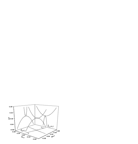
Figure 1: The curves $\hat{C}_{n}(\pi_{1})$ and $\hat{C}_{n+1}(\pi_{1})$ are the trajectories traced by the points $\hat{\cal E}_{n}(\xi_{1},\bar{\xi}_{2}^{(1)})$ and $\hat{\cal E}_{n+1}(\xi_{1},\bar{\xi}_{2}^{(1)})$ on the hypersurface $\hat{\cal E}_{n,n+1}(\xi_{1},\bar{\xi}_{2}^{(1)})$ when the point $(\xi_{1},\bar{\xi}_{2}^{(1)})$ moves along the straight line path $\pi_{1}$ in parameter space. In the figure, the path $\pi_{1}$ runs parallel to the vertical axis and crosses the line ${\cal L}_{I}$ at a point $(\xi_{1,c},\bar{\xi}_{2}^{(1)})$ with $\xi_{1,c}<\xi_{1}^{*}$ and $\bar{\xi}_{2}^{(1)}<\xi^{*}_{2}$. The projections of $\hat{C}_{n}(\pi_{1})$ and $\hat{C}_{n+1}(\pi_{1})$ on the plane $(Im{\cal E},\xi_{1})$ are sections of the surface $S_{I}$; the projections of $\hat{C}_{n}(\pi_{1})$ and $\hat{C}_{n+1}(\pi_{1})$ on the plane $(Re{\cal E},\xi_{1})$ are sections of the surface $S_{R}$. The projections of $\hat{C}_{n}(\pi_{1})$ and $\hat{C}_{n+1}(\pi_{1})$ on the plane $(Re{\cal E},Im{\cal E})$ are the trajectories of the $S-$matrix poles in the complex energy plane. In the figure, $d-d^{*}=\xi_{1}$

.

To relate the geometrical properties of this intersection with the experimentally determined properties of crossings and anticrossings of energies and widths, let us consider a point $(\xi_{1},\bar{\xi}_{2}^{(i)})$ in parameter space away from the exceptional point. To this point corresponds the pair of non-degenerate resonance energy eigenvalues ${\cal E}_{n}(\xi_{1},\bar{\xi}_{2}^{(i)})$ and ${\cal E}_{n+1}(\xi_{1},\bar{\xi}_{2}^{(i)})$, represented by two points on the hypersurface $\hat{\epsilon}_{n,n+1}(\xi_{1},\xi_{2})$. As the point $(\xi_{1},\bar{\xi}_{2}^{(i)})$ moves on a straight line path $\pi_{i}$ in parameter space,

$$\pi_{i}:\hskip 5.69046pt\xi_{1,i}\leq\xi_{1}\leq\xi_{1,f},\ \ \xi_{2}=\bar{\xi}_{2}^{(i)}$$ (40)

the corresponding points, ${\cal E}_{n}(\xi_{1},\bar{\xi}^{(i)}_{2})$ and ${\cal E}_{n+1}(\xi_{1},\bar{\xi}_{2}^{(i)})$ trace two curving trajectories, $\hat{C}_{n}(\pi_{1})$ and $\hat{C}_{n+1}(\pi_{1})$ on the $\hat{\epsilon}_{n,n+1}(\xi_{1},\xi_{2})$ hypersurface. Since $\xi_{2}$ is kept constant at the fixed value $\bar{\xi}_{2}^{(i)}$, the trajectories (sections) $\hat{C}_{n}(\pi_{i})$ and $\hat{C}_{n+1}(\pi_{i})$, may be represented as three-dimensional curves in a space ${\cal E}_{3}$ with cartesian coordinates $(Re\epsilon,Im\epsilon,\xi_{1})$, see Figs. 1,2 and 3.

Figure 2: The curves $\hat{C}_{n}(\pi_{2})$ and $\hat{C}_{n+1}(\pi_{2})$ are the trajectories of the points $\hat{\cal E}_{n}(\xi_{1},\xi^{*}_{2})$ and $\hat{\cal E}_{n+1}(\xi_{1},\xi^{*}_{2})$ on the hypersurface $\hat{\cal E}_{n,n+1}(\xi_{1},\xi_{2})$ when the point $(\xi_{1},\xi^{*}_{2})$ moves along a straight line path $\pi_{2}$ that goes through the exceptional point $(\xi^{*}_{1},\xi^{*}_{2})$ in parameter space. The projections of $\hat{C}_{n}(\pi_{2})$ and $\hat{C}_{n+1}(\pi_{2})$ on the planes $(Re{\cal E},\xi_{1})$ and $(Im{\cal E},\xi_{1})$ are sections of the surfaces $S_{R}$ and $S_{I}$ respectively, and show a joint crossing of energies and widths. The projections of $\hat{C}_{n}(\pi_{2})$ and $\hat{C}_{n+1}(\pi_{2})$ on the plane $(Re{\cal E},Im{\cal E})$ are two straight line trajectories of the $S-$matrix poles crossing at 90^∘ in the complex energy plane. At the crossing point, the two simple poles coalesce into one double pole of $S(E)$.

Figure 3: The curves $\hat{C}_{n}(\pi_{3})$ and $\hat{C}_{n+1}(\pi_{3})$ are the trajectories traced by the points $\hat{\cal E}_{n}(\xi_{1},\bar{\xi}^{(3)}_{2})$ and $\hat{\cal E}_{n+1}(\xi_{1},\bar{\xi}^{(3)}_{2})$ on the hypersurface ${\cal E}_{n,n+1}(\xi_{1},\bar{\xi}_{2}^{(3)})$ when the point $(\xi_{1},\bar{\xi}^{(3)}_{2})$ moves along a straight line path $\pi_{3}$ going trough the point $({\xi}_{1,c},\bar{\xi}^{(3)}_{2})$ with ${\xi}_{1,c}>\xi^{*}_{1}$. The path $\pi_{3}$ crosses the line ${\cal L}_{R}$. The projections of $\hat{C}_{n}(\pi_{3})$ and $\hat{C}_{n+1}(\pi_{3})$ on the plane $(Re{\cal E},\xi_{1})$ show a crossing, but the projections on the planes $(Im{\cal E},\xi_{1})$ and $(Re{\cal E},Im{\cal E})$ do not cross. In the figure, $\xi_{1}=d-d^{*}$.

The projections of the curves $\hat{C}_{n}(\pi_{i})$ and $\hat{C}_{n+1}(\pi_{i})$ on the planes $(Re\epsilon,\xi_{1})$ and $(Im\epsilon,\xi_{1})$ are

$$Re[\hat{C}_{m}(\pi_{i})]=Re\hat{\cal E}_{m}(\xi_{1},\bar{\xi}_{2}^{(i)})\ \ m=n,n+1$$ (41)

and

$$Im[\hat{C}_{m}(\pi_{i})]=Im\hat{\cal E}_{m}(\xi_{1},\bar{\xi}^{(i)}_{2})\ \ m=n,n+1$$ (42)

respectively.

From eqs.(23-25), and keeping $\xi_{2}=\bar{\xi}^{(i)}_{2}$, we obtain

$$\begin{array}[]{c}\Delta E=E_{n}-E_{n+1}=\Bigl{(}Re\hat{\cal E}_{n}-Re\hat{\cal E}_{n+1}\Bigr{)}\Bigr{|}_{\xi_{2}=\bar{\xi}_{2}^{(i)}}\cr=\frac{\sigma^{(n)}\sqrt{2}}{2}\Bigl{[}{}_{+}\sqrt{(\vec{R}\cdot\vec{\xi})^{2}+(\vec{I}\cdot\vec{\xi})^{2}}+(\vec{R}\cdot\vec{\xi})\Bigr{]}^{1/2}\Bigr{]}_{\xi_{2}=\bar{\xi}_{2}^{(i)}}\end{array}$$ (43)

and

$$\begin{array}[]{c}\Delta\Gamma=\frac{1}{2}\Bigl{(}\Gamma_{n}-\Gamma_{n+1}\Bigr{)}=Im\Bigl{(}{\cal E}_{n+1}\Bigr{)}-\Bigl{(}Im{\cal E}_{n}\Bigr{)}\cr=\frac{\sigma^{(n)}_{I}\sqrt{2}}{2}\Bigl{[}{}_{+}\sqrt{(\vec{R}\cdot\vec{\xi})^{2}+(\vec{I}\cdot\vec{\xi})^{2}}-(\vec{R}\cdot\vec{\xi})\Bigr{]}^{1/2}\Bigr{|}_{\xi_{2}=\bar{\xi}_{2}^{(i)}}\end{array}$$ (44)

These expressions allow us to relate the terms $(\vec{R}\cdot\vec{\xi})$ and $(\vec{I}\cdot\vec{\xi})$ directly with observables of the isolated doublet of resonances. Taking the product of $\Delta E\Delta\Gamma$, and recalling eq.(21), we get

$$\Delta E\Delta\Gamma=\Bigl{(}\vec{I}\cdot\vec{\xi}\Bigr{)}\Bigr{|}_{\xi_{2}=\bar{\xi}_{2}^{(i)}}$$ (45)

and taking the differences of the squares of the left hand sides of (43) and (44), we get

$$\Bigl{(}\Delta E\Bigr{)}^{2}-\frac{1}{4}\Bigl{(}\Delta\Gamma\Bigr{)}^{2}=\Bigl{(}\vec{R}\cdot\vec{\xi}\Bigr{)}\Bigr{|}_{\xi_{2}=\bar{\xi}_{2}^{(i)}}$$ (46)

At a crossing of energies $\Delta E$ vanishes, and at a crossing of widths $\Delta\Gamma$ vanishes. Hence, the relation found in eq.(45) means that a crossing of energies or widths can occur if and only if $(\vec{I}\cdot\vec{\xi})_{\bar{\xi}^{(i)}_{2}}$ vanishes

For a vanishing $(\vec{I}\cdot\vec{\xi}_{c})_{\bar{\xi}^{(i)}_{2}}=0=\Delta E\Delta\Gamma$, we find three cases, which are distinguished by the sign of $(\vec{R}\cdot\vec{\xi}_{c})_{\bar{\xi}^{(i)}_{2}}$. From eqs. (43) and (44),

1. $(\vec{R}\cdot\vec{\xi}_{c})_{\bar{\xi}^{(i)}_{2}}>0$ implies $\Delta E\neq 0$ and $\Delta\Gamma=0$, i.e. energy anticrossing and width crossing.

2. $(\vec{R}\cdot\vec{\xi}_{c})_{\bar{\xi}^{(i)}_{2}}=0$ implies $\Delta E=0$ and $\Delta\Gamma=0$, that is, joint energy and width crossings, which is also degeneracy of the two complex resonance energy eigenvalues.

3. $(\vec{R}\cdot\vec{\xi}_{c})_{\bar{\xi}^{(i)}_{2}}<0$ implies $\Delta E=0$ and $\Delta\Gamma\neq 0$, i.e. energy crossing and width anticrossing.

This rich physical scenario of crossings and anticrossings for the energies and widths of the complex resonance energy eigenvalues, extends a theorem of von Neumann and Wigner wigner for bound states to the case of unbound states.

The general character of the crossing-anticrossing relations of the energies and widths of a mixing isolated doublet of resonances, discussed above, has been experimentally established by P. von Brentano and his collaborators in a series of beautiful experiments Brent1 ; Phil ; Brent2 .

A detailed account of these and other results will be published elsewhere hern5 ; hern6

V Summary and conclusions

We developed the theory of the unfolding of the energy eigenvalue surfaces close to a degeneracy point (exceptional point) of two unbound states of a Hamiltonian depending on control parameters. From the knowledge of the Jost function, as function of the control parameters of the system, we derived a 2-parameter family of functions which is contact equivalent to the exact energy-pole position function at the exceptional point and includes all small perturbations of the degeneracy conditions. A simple and explicit, but very accurate, representation of the eigenenergy surfaces close to the exceptional point is obtained. In parameter space, the hypersurface representing the complex resonance energy eigenvalues has an algebraic branch point of rank one, and branch cuts in its real and imaginary parts extending in opposite directions in parameter space. The rich phenomenology of crossings and anticrossings of the energies and widths of the resonances of an isolated doublet of unbound states of a quantum system, observed when one control parameter is varied and the other is kept constant, is fully explained in terms of the local topology of the eigenenergy hypersurface in the vecinity of the crossing point.

References

(1)E. Hernández, A. Jáuregui and A. Mondragón,
Rev. Mex. Fis. 38, Suppl 2, 128-145 (1992)
(2)A. Mondragón and E. Hernández, J. Phys. A:
Math. and Gen. 26, 5595-5611, (1993).
(3)A. Mondragón and E. Hernández, J. Phys. A:
Math. and Gen. 29, 2567-2585, (1996).
(4)A. Mondragón and E. Hernández, in Irreversibility and Causality: Semigroup and Rigged Hilbert
Space, edited by A. Bohm, D.-H. Doebner, and P. Kielanowski,
Lecture Notes in Physics.Vol. 504
(Springer-Verlag Berlin, 1998) p 257-278.
(5)W. D. Heiss, Eur. Phys. D 7, 1-4, (1999).
(6)P. von Brentano and M. Philipp, Phys. Lett. B 454, 171-175, (1999).
(7)M. Philipp, P. von Brentano, G. Pascovici and A. Richter,
Phys. Rev. E 62, 1922-1926, (2000)