Van der Waals interaction between microparticle and uniaxial crystal with application to hydrogen atoms and multiwall carbon nanotubes

Abstract

The Lifshitz theory of the van der Waals force is extended for the case of an atom (molecule) interacting with a plane surface of an uniaxial crystal or with a long solid cylinder or cylindrical shell made of isotropic material or uniaxial crystal. For a microparticle near a semispace or flat plate made of an uniaxial crystal the exact expressions for the free energy of the van der Waals and Casimir-Polder interaction are presented. An approximate expression for the free energy of microparticle-cylinder interaction is obtained which becomes precise for microparticle-cylinder separations much smaller than cylinder radius. The obtained expressions are used to investigate the van der Waals interaction between hydrogen atoms (molecules) and graphite plates or multiwall carbon nanotubes. To accomplish this the behavior of graphite dielectric permittivities along the imaginary frequency axis is found using the optical data for the complex refractive index of graphite for the ordinary and extraordinary rays. It is shown that the position of hydrogen atoms inside multiwall carbon nanotubes is energetically preferable compared with outside.

I Introduction

The van der Waals interaction between microparticle and macrobody has long been investigated. It is of much importance for understanding of a large body of physical and chemical phenomena connected with atom-surface interaction including adsorption and friction. In a pioneering work in Ref. 1 , the interaction potential between an atom at a separation $a$ from a plane wall was found in the from $V_{3}(a)=-C_{3}/a^{3}$. This result is applicable at separations less than a few nanometers. More recently, a lot of different atoms, molecules and wall materials was studied. In particular, in Refs. 1a ; 1b the values of $C_{3}$ were computed for the interaction of H, H₂, He, Ne, Ar, Cr, Xe, and CH₄ with the planar surfaces of insulators (sapphire, LiF, CaF₂, and boron nitride). At much greater separations the atom-wall interaction is described by the Casimir-Polder potential $V_{4}(a)=-C_{4}/a^{4}$ 2 taking relativistic effects into account. The complete theory of the van der Waals atom-wall interaction at nonzero temperature is given by the Lifshitz formula 3 in terms of the dynamic polarizability of an atom (molecule) and the frequency-dependent dielectric permittivity of wall material. The potentials $V_{3}(a)$ and $V_{4}(a)$, obtained previously, are the two limiting cases of this formula.

During the last few years van der Waals forces have found important new applications in experiments on quantum reflection and diffraction of ultra-cold atoms on different surfaces 4 ; 5 ; 6 ; 7 and in Bose-Einstein condensation 8 ; 9 . In connection with this, the detailed examination of different corrections to the Casimir-Polder and van der Waals interactions, including the precise effect of atomic polarizability and nonideality of wall material was performed in Refs. 10 ; 10a . Effectively this resulted in the investigation of accurate dependences of the coefficients $C_{3}$ and $C_{4}$ on separation and temperature.

Although the Lifshitz theory presents considerable opportunity for extensive studies of the van der Waals force 11 ; 12 , it is essentially restricted by macroscopic bodies with plane boundaries. The use of approximations, like the proximity force theorem 13 , permitted one to obtain rather precise results for a large sphere near a plane plate, a configuration frequently used in recent experiments on measuring the Casimir force 14 ; 15 ; 16 ; 17 ; 18 . In most cases the macrobodies with plane boundaries were supposed to be isotropic.

In the present paper we generalize the Lifshitz formula for a microparticle situated near the surface of an uniaxial crystal. Both cases of crystal semispace with plane boundary and a plane plate of finite thickness are considered. As a next step, we derive the approximate expression for the free energy of the van der Waals interaction between a microparticle and a solid cylinder or cylindrical shell made of an uniaxial crystal. In the limiting case this expression is applicable to a microparticle near a cylinder made of an isotropic material with frequency dependent dielectric permittivity (a configuration which also has not been investigated previously). We apply the obtained results to investigate the van der Waals interaction between hydrogen atoms or molecules and graphite plates or multiwall carbon nanotubes.

The study of the van der Waals interaction between hydrogen atoms and a graphitic surface has become urgent after the proposal of Ref. 19 to use the singlewall carbon nanotubes for hydrogen storage. Since, many papers were published on the use of both singlewall and multiwall nanotubes for hydrogen storage and containing both promising and disappointing results (see Ref. 20 for review). The macroscopic theoretical approach leads to a conclusion 21 that the carbon nanostructures might absorb hydrogen from 4 to 14 percent of their weight. However, the microscopic mechanisms responsible for this absorption are still unknown. The van der Waals forces acting between hydrogen atoms or molecules and carbon nanostructures, which might play an important role in absorption phenomena, are practically unexplored. Some preliminary results for graphite sheets and singlewall nanotubes can be found in Refs. 22 and 23 ; 23a , respectively. The van der Waals interaction of fulerene molecules and adsorption of these molecules on graphite were considered in Ref. 23b .

To apply the Lifshitz-type formulas for the van der Waals free energy, obtained in the paper, to the case of hydrogen atoms and molecules near graphite surface, we calculate the dielectric permittivities of graphite and dynamic polarizabilities of hydrogen atom and molecule along the imaginary frequency axis. To do this, we discuss different sets of tabulated optical data for the complex refractive index of graphite and use the most reliable ones to perform the Kramers-Kronig analysis. The van der Waals interactions between hydrogen atom and molecule and graphite semispace or plate of finite thickness are calculated. The free energies of hydrogen atom inside and outside of a multiwall carbon nanotube are found as functions of an atom-nanotube separation distance and internal and external nanotube radia. The location of a hydrogen atom inside a multiwall nanotube is demonstrated to be preferable from an energetic point of view.

The paper is organized as follows. In Sec. II we present the Lifshitz formula for the van der Waals (and Casimir-Polder) interaction between microparticle and plane surface of an uniaxial crystal. Sec. III contains derivation of general expression for the van der Waals free energy of a microparticle external to a solid cylinder or cylindrical shell made of an uniaxial crystal. In Sec. IV the dielectric permittivities of graphite and the atomic and molecular dynamic polarizabilities of hydrogen along the imaginary frequency axis are obtained. In Sec. V calculation results are presented for the van der Waals interaction between hydrogen atom or molecule and graphite semispace or a plane plate of finite thickness. In Sec. VI the same is done for hydrogen atom or molecule external to a multiwall carbon nanotube. Comparison between the free energies of hydrogen atom inside and outside multiwall nanotube is done in Sec. VII. Sec. VIII contains our discussion and conclusions.

II Lifshitz formula for the van der Waals interaction
between microparticle and plane surface of an uniaxial crystal

First we consider a neutral microparticle (atom or molecule) with a dynamic polarizability $\alpha(\omega)$ at separation $a$ from a plane surface of the isotropic semispace with dielectric permittivity $\varepsilon(\omega)$ at temperature $T$ in thermal equilibrium. In this case the free energy of microparticle-semispace van der Waals interaction is given by the familiar Lifshitz formula 3 (see also 9 ; 10 ; 24 ; 25 ; 26 )

$$F_{E}^{s}(a,T)=-k_{B}T\sum\limits_{l=0}^{\infty}{\vphantom{\sum}}^{\prime}\alpha(i\xi_{l})\int_{0}^{\infty}k_{\bot}dk_{\bot}q_{l}e^{-2aq_{l}}$$

$$\phantom{aaa}\times\left\{2r_{\|}^{s}(\xi_{l},k_{\bot})+\frac{\xi_{l}^{2}}{q_{l}^{2}c^{2}}\left[r_{\bot}^{s}(\xi_{l},k_{\bot})-r_{\|}^{s}(\xi_{l},k_{\bot})\right]\right\}.$$ (1)

Here $\xi_{l}=2\pi k_{B}Tl/\hbar$ are the Matsubara frequencies, $k_{B}$ is the Boltzmann constant, $l=0,\,1,\,2,\,\ldots\,$, and $k_{\bot}$ is the magnitude of a wave vector component in the plane surface of a semispace. The coefficients of reflection for two independent polarizations of electromagnetic field are given by

$$r_{\|}^{s}(\xi_{l},k_{\bot})=\frac{\varepsilon_{l}q_{l}-k_{l}}{\varepsilon_{l}q_{l}+k_{l}},$$

$$r_{\bot}^{s}(\xi_{l},k_{\bot})=\frac{k_{l}-q_{l}}{k_{l}+q_{l}},$$ (2)

where

$$q_{l}=\sqrt{k_{\bot}^{2}+\frac{\xi_{l}^{2}}{c^{2}}},\quad k_{l}=\sqrt{k_{\bot}^{2}+\varepsilon_{l}\frac{\xi_{l}^{2}}{c^{2}}},$$

$$\varepsilon_{l}=\varepsilon(i\xi_{l}),$$ (3)

and prime near the summation sign in Eq. (1) means that the term for $l=0$ has to be multiplied by 1/2.

Eq. (1) can be readily generalized for the case when the microparticle is located not near a semispace, but near a flat plate of some finite thickness $d$ with the same dielectric permittivity $\varepsilon(\omega)$. In this case the free energy of the van der Waals interaction $F_{E}^{p}(a,T)$ again is given by Eq. (1) where, however, the reflection coefficients from a semispace $r_{\|,\bot}^{s}(\xi_{l},k_{\bot})$ should be replaced by the reflection coefficients from a plate of finite thickness $r_{\|,\bot}^{p}(\xi_{l},k_{\bot})$. The explicit expressions for them are obtained from the free energy of the van der Waals interaction between the layered media (see, e.g., 24 ; 27 ; 28 ):

$$r_{\|}^{p}(\xi_{l},k_{\bot})=\frac{\varepsilon_{l}^{2}q_{l}^{2}-k_{l}^{2}}{\varepsilon_{l}^{2}q_{l}^{2}+k_{l}^{2}+2q_{l}k_{l}\varepsilon_{l}\mbox{coth}(k_{l}d)},$$

$$r_{\bot}^{p}(\xi_{l},k_{\bot})=\frac{k_{l}^{2}-q_{l}^{2}}{k_{l}^{2}+q_{l}^{2}+2q_{l}k_{l}\mbox{coth}(k_{l}d)}.$$ (4)

In the limit $d\to\infty$ Eq. (4) transforms into Eq. (2).

Let us now consider a semispace or a plate of finite thickness made of an uniaxial crystal (graphite for instance) which is characterized by two dissimilar dielectric permittivities $\varepsilon_{x}(\omega)=\varepsilon_{y}(\omega)$ and $\varepsilon_{z}(\omega)$. Let a microparticle be located near the uniaxial crystal semispace restricted by the plane $(x,y)$, and the crystal optical axis $z$ being perpendicular to it. Then the free energy of the van der Waals interaction is again given by Eq. (1) where the coefficients of reflection from the surface of isotropic semispace $r_{\|,\bot}^{s}(\xi_{l},k_{\bot})$ should be replaced by their generalization for the case of uniaxial crystal (graphite) 29 :

$$r_{\|;g}^{s}(\xi_{l},k_{\bot})=\frac{\sqrt{\varepsilon_{xl}\varepsilon_{zl}}q_{l}-k_{zl}}{\sqrt{\varepsilon_{xl}\varepsilon_{zl}}q_{l}+k_{zl}},$$

$$r_{\bot;g}^{s}(\xi_{l},k_{\bot})=\frac{k_{xl}-q_{l}}{k_{xl}+q_{l}}.$$ (5)

Here the following notations are introduced

$$k_{xl}=\sqrt{k_{\bot}^{2}+\varepsilon_{xl}\frac{\xi_{l}^{2}}{c^{2}}},\qquad k_{zl}=\sqrt{k_{\bot}^{2}+\varepsilon_{zl}\frac{\xi_{l}^{2}}{c^{2}}},$$

$$\varepsilon_{xl}=\varepsilon_{x}(i\xi_{l}),\qquad\varepsilon_{zl}=\varepsilon_{z}(i\xi_{l}).$$ (6)

For isotropic crystal $\varepsilon_{x}=\varepsilon_{z}=\varepsilon$ and Eq. (5) coincides with Eq. (2).

If a microparticle is located near a flat plate of finite thickness made of uniaxial crystal ($z$-axis is perpendicular to the plate), the free energy $F_{E}^{p}(a,T)$ is given again by Eq. (1), where the coefficients of reflection from an isotropic plate $r_{\|,\bot}^{p}(\xi_{l},k_{\bot})$ are replaced by the reflection coefficients from a plate made of uniaxial crystal:

$$r_{\|;g}^{p}(\xi_{l},k_{\bot})=\frac{{\varepsilon_{xl}\varepsilon_{zl}}q_{l}^{2}-k_{zl}^{2}}{{\varepsilon_{xl}\varepsilon_{zl}}q_{l}^{2}+k_{zl}^{2}+2\sqrt{\varepsilon_{xl}\varepsilon_{zl}}q_{l}k_{zl}\mbox{coth}(k_{zl}d)},$$

$$r_{\bot;g}^{p}(\xi_{l},k_{\bot})=\frac{k_{xl}^{2}-q_{l}^{2}}{k_{xl}^{2}+q_{l}^{2}+2q_{l}k_{xl}\mbox{coth}(k_{xl}d)}.$$ (7)

For the anisotropic plate of infinite thickness ($d\to\infty$) Eq. (7) transforms into Eq. (5). On the other hand, in the limit of the plate made of isotropic substance Eq. (7) coincides with Eq. (4).

Eq. (1) with reflection coefficients (5), (7) is used in Sec.V for computations of the van der Waals interaction between the hydrogen atoms or molecules and the plane surface of a semispace or a plate made of graphite.

III Free energy of the van der Waals interaction for
a microparticle external to a solid or hollow cylinder

In this section we derive the Lifshitz-type formula for the van der Waals free energy of a microparticle located at a separation $a$ from the external surface of a solid cylinder or cylindrical shell made of an uniaxial crystal. It is assumed that the crystal optical axis $z$ is perpendicular to the cylinder surface of crystalline layers. The outer radius of a cylinder is $R$ and the thickness of a crystal cylindrical shell is $d\leq R$. In the case $d=R$ the cylinder is solid. If $d<R$, there is an empty cylindrical cavity inside of a cylinder. As in the previous section, the crystalline material of the cylindrical shell is described by the dielectric permittivities $\varepsilon_{x}(\omega)$ and $\varepsilon_{z}(\omega)$. The derivation presented below is based on the same approach which was previously used in literature 3 ; 10 ; 24 ; 25 ; 26 to derive the Lifshitz formula for microparticle-semispace (plate) interaction from the Lifshitz formula for a configuration of two parallel semispaces (plates).

Let us consider an infinite space filled with an isotropic substance having a dielectric permittivity $\varepsilon(\omega)$, containing an empty cylindrical cavity of radius $R+a$. We introduce our solid cylinder or cylindrical shell of external radius $R$ made of an uniaxial crystal inside this cavity so that the cylinder axis coincides with the axis of the cavity (see Fig. 1). Then there is a gap of thickness $a$ between our cylinder and the boundary of the cylindrical cavity of radius $R+a$ restricting the infinite space with the dielectric permittivity $\varepsilon(\omega)$. Each element of our cylinder experiences an attractive van der Waals interaction on the source side of the boundary of the cylindrical cavity restricting the infinite space. With the help of the proximity force theorem the free energy of this interaction between two cylinders can be approximately represented in the form (see Ref. 30 for the case of ideal metals)

$$F_{E}^{c,c}(a,T)=2\pi L\sqrt{R(R+a)}F_{E}^{i,s}(a,T).$$ (8)

Here $F_{E}^{i,s}(a,T)$ is the free energy per unit area in the configuration either of two semispaces separated by a gap of width $a$ (in this case $i=s$, our cylinder is solid, one semispace is filled with an uniaxial crystal and the other is filled with a material of dielectric permittivity $\varepsilon(\omega)$) or of a flat plate of thickness $d$ and a semispace separated by the same gap (in this case $i=p$, and we are dealing with cylindrical shell having a longitudinal hole of radius $R-d$; the plate is made of an uniaxial crystal and semispace of material with a dielectric permittivity $\varepsilon(\omega)$). In Eq. (8) $L$ is the length of our solid or hollow cylinder which is supposed to be much larger than its radius $R$.

As shown in Ref. 30 (see also Ref. 31 ), the accuracy of Eq. (8) is rather high. For example, within the separation region $0<a<R/2$ the results calculated by Eq. (8) coincide with the exact ones up to 1% in the case of cylinders made of perfect metal (for other materials the accuracy may be different for only a fraction of percent). This is quite satisfactory for application to multiwall nanotubes with $R$ of about a few ten nanometers considered below.

The explicit expressions for the free energy $F_{E}^{i,s}(a,T)$ are well known 3 ; 24 ; 25 ; 26 ; 27 ; 28

$$F_{E}^{i,s}(a,T)=\frac{k_{B}T}{2\pi}\sum\limits_{l=0}^{\infty}{\vphantom{\sum}}^{\prime}\int_{0}^{\infty}k_{\bot}dk_{\bot}\left\{\ln\left[1-r_{\|;g}^{s,p}(\xi_{l},k_{\bot})r_{\|}^{s}(\xi_{l},k_{\bot})e^{-2aq_{l}}\right]\right.$$

$$\phantom{aaaaa}+\left.\ln\left[1-r_{\bot;g}^{s,p}(\xi_{l},k_{\bot})r_{\bot}^{s}(\xi_{l},k_{\bot})e^{-2aq_{l}}\right]\right\}.$$ (9)

Here the reflection coefficients $r_{\|,\bot;g}^{s}$ from the semispace of uniaxial crystal are given by Eq. (5), coefficients $r_{\|,\bot;g}^{p}$, describing reflection from a flat plate of uniaxial crystal, are given by Eq. (7), and coefficients $r_{\|,\bot}^{s}$ describing reflection from isotropic semispace are presented in Eq. (2). Notice that when index $i$ in the left-hand side of Eq. (9) is equal to $s$ or $p$ one should choose $s$ or $p$ in the right-hand side, respectively.

To continue with our derivation, we now suppose that the isotropic substance with the dielectric permittivity $\varepsilon(\omega)$ is rarefied with the number $N$ of atoms or molecules per unit volume. Expanding the quantity $F_{E}^{c,c}(a,T)$ from the left-hand side of Eq. (8) as a power series in $N$ and using the additivity of the first-order term, one can write

$$F_{E}^{c,c}(a,T)=N\int_{a}^{\infty}F_{E}^{c}(z,T)2\pi(R+z)Ldz+O(N^{2}),$$ (10)

where $F_{E}^{c}(z,T)$ is the free energy of the van der Waals interaction of a single atom belonging to an isotropic substance with a solid cylinder or cylindrical shell made of an uniaxial crystal (note that separation $z$ is measured from the external surface of the cylinder in the direction perpendicular to it).

By differentiation of both sides of Eq. (10) with respect to $a$, we obtain

$$-\frac{\partial F_{E}^{c,c}(a,T)}{\partial a}=2\pi(R+a)LNF_{E}^{c}(a,T)+O(N^{2}).$$ (11)

The same derivative can be found when differentiating both sides of Eq. (8)

$$-\frac{\partial F_{E}^{c,c}(a,T)}{\partial a}=2\pi L\sqrt{R(R+a)}$$ (12)

$$\phantom{aaaaaaaa}\times\left[-\frac{1}{2(R+a)}F_{E}^{i,s}(a,T)+F^{i,s}(a,T)\vphantom{\frac{1}{2(R+a)}}\right],$$

where

$$F^{i,s}(a,T)=-\frac{\partial F_{E}^{i,s}(a,T)}{\partial a}$$ (13)

is the van der Waals force per unit area acting between the semispace made of an uniaxial crystal ($i=s$) or a flat plate made of the same material and a semispace with a dielectric permittivity $\varepsilon$. The expression for this force is easily obtained from Eqs. (9) and (13):

$$F^{i,s}(a,T)=-\frac{k_{B}T}{\pi}\sum\limits_{l=0}^{\infty}{\vphantom{\sum}}^{\prime}\int_{0}^{\infty}k_{\bot}dk_{\bot}q_{l}$$ (14)

$$\phantom{aaaa}\times\left[\frac{r_{\|;g}^{s,p}(\xi_{l},k_{\bot})r_{\|}^{s}(\xi_{l},k_{\bot})}{e^{2aq_{l}}-r_{\|;g}^{s,p}(\xi_{l},k_{\bot})r_{\|}^{s}(\xi_{l},k_{\bot})}+\frac{r_{\bot;g}^{s,p}(\xi_{l},k_{\bot})r_{\bot}^{s}(\xi_{l},k_{\bot})}{e^{2aq_{l}}-r_{\bot;g}^{s,p}(\xi_{l},k_{\bot})r_{\bot}^{s}(\xi_{l},k_{\bot})}\right].$$

The dielectric permittivity of a rarefied substance can be expanded in Taylor series in powers of $N$ 32

$$\varepsilon(i\xi_{l})=1+4\pi\alpha(i\xi_{l})N+O(N^{2}),$$ (15)

where $\alpha(\omega)$ is the dynamic polarizability of an atom (molecule) of this substance. Substituting Eq. (15) in Eqs. (2) and (3) we obtain

$$r_{\|}^{s}(\xi_{l},k_{\bot})=\pi\alpha(i\xi_{l})N\left(2-\frac{\xi_{l}^{2}}{q_{l}^{2}c^{2}}\right)+O(N^{2}),$$

$$r_{\bot}^{s}(\xi_{l},k_{\bot})=\pi\alpha(i\xi_{l})\frac{N\xi_{l}^{2}}{q_{l}^{2}c^{2}}+O(N^{2}).$$ (16)

Using Eq. (16), the free energy $F_{E}^{i,s}$ and the force $F^{i,s}$ from Eqs. (9) and (14) can be represented in the form

$$F_{E}^{i,s}(a,T)=-\frac{k_{B}TN}{2}\sum\limits_{l=0}^{\infty}{\vphantom{\sum}}^{\prime}\alpha(i\xi_{l})\int_{0}^{\infty}k_{\bot}dk_{\bot}$$

$$\phantom{aaa}\times\left[\left(2-\frac{\xi_{l}^{2}}{q_{l}^{2}c^{2}}\right)r_{\|;g}^{s,p}(\xi_{l},k_{\bot})+\frac{\xi_{l}^{2}}{q_{l}^{2}c^{2}}r_{\bot;g}^{s,p}(\xi_{l},k_{\bot})\right]e^{-2aq_{l}}+O(N^{2}),$$

(17)

$$F^{i,s}(a,T)=-k_{B}TN\sum\limits_{l=0}^{\infty}{\vphantom{\sum}}^{\prime}\alpha(i\xi_{l})\int_{0}^{\infty}k_{\bot}dk_{\bot}q_{l}$$

$$\phantom{aaa}\times\left[\left(2-\frac{\xi_{l}^{2}}{q_{l}^{2}c^{2}}\right)r_{\|;g}^{s,p}(\xi_{l},k_{\bot})+\frac{\xi_{l}^{2}}{q_{l}^{2}c^{2}}r_{\bot;g}^{s,p}(\xi_{l},k_{\bot})\right]e^{-2aq_{l}}+O(N^{2}).$$

Substituting Eq. (17) in Eq. (12), one finds

$$-\frac{\partial F_{E}^{c,c}(a,T)}{\partial a}=-2\pi LNk_{B}T\sqrt{R(R+a)}\sum\limits_{l=0}^{\infty}{\vphantom{\sum}}^{\prime}\alpha(i\xi_{l})\int_{0}^{\infty}k_{\bot}dk_{\bot}\left[q_{l}-\frac{1}{4(R+a)}\right]$$

$$\times\left\{2r_{\|;g}^{s,p}(\xi_{l},k_{\bot})+\frac{\xi_{l}^{2}}{q_{l}^{2}c^{2}}\left[r_{\bot;g}^{s,p}(\xi_{l},k_{\bot})-r_{\|;g}^{s,p}(\xi_{l},k_{\bot})\right]\right\}e^{-2aq_{l}}+O(N^{2}).$$ (18)

As a final stage of the derivation, we substitute the result (18) into the left-hand side of Eq. (11), take the limit $N\to 0$ and arrive at desired expression for the free energy of van der Waals interaction between a microparticle and a cylinder made of uniaxial crystal

$$F_{E}^{c}(a,T)=-k_{B}T\sqrt{\frac{R}{R+a}}\sum\limits_{l=0}^{\infty}{\vphantom{\sum}}^{\prime}\alpha(i\xi_{l})\int_{0}^{\infty}k_{\bot}dk_{\bot}e^{-2aq_{l}}\left[q_{l}-\frac{1}{4(R+a)}\right]$$

$$\phantom{aaa}\times\left\{2r_{\|;g}^{s,p}(\xi_{l},k_{\bot})+\frac{\xi_{l}^{2}}{q_{l}^{2}c^{2}}\left[r_{\bot;g}^{s,p}(\xi_{l},k_{\bot})-r_{\|;g}^{s,p}(\xi_{l},k_{\bot})\right]\right\}.$$ (19)

In the case of a solid cylinder, the reflection coefficients $r_{\|,\bot;g}^{s}$, given by Eq. (5), should be chosen in the right-hand side of Eq. (19). For a cylindrical shell, coefficients $r_{\|,\bot;g}^{p}$ from Eq. (7) should be used. Notice that in the limit $R\to\infty$ Eq. (19) coincides with a known result (1) for the free energy of microparticle near a plane surface of a semispace. The above derivation is preserved also in the limiting case of a solid or hollow cylinder made of isotropic material with $\varepsilon_{x}=\varepsilon_{y}=\varepsilon_{z}\equiv\varepsilon$. To obtain the result for isotropic cylinder, one should substitute in Eq. (19) the reflection coefficients (2), (4) instead of (5), (7).

Eq. (19) is the approximate one. It is, however, practically exact at $a\ll R$ and is of high precision (the error is of about 1%) at all separations $a\leq R/2$. That is why this equation is reliable for calculations of the van der Waals interaction between a cylinder and microparticles located in its close proximity.

IV Dielectric permittivities of graphite and dynamic
polarizabilities of hydrogen atom and molecule along the imaginary frequency axis

Below we used the Lifshitz-type formulas obtained above to calculate the van der Waals interaction between hydrogen atoms or molecules and graphite semispace or flat plate [Eqs. (1), (5), (7)] or graphite cylinder [Eqs. (5), (7), (19)]. The graphite cylinder models a multiwall carbon nanotube (see Sec. VI). To attain these ends, one needs the values of dynamic polarizabilities of hydrogen atom and molecule and also both dielectric permittivities of graphite at all Matsubara frequencies which give non-negligible contribution to the result.

The precise expression for the atomic dynamic polarizability of hydrogen is given by the 10-oscillator formula 33 written in atomic units

$$\alpha(i\xi_{l})=\sum\limits_{j=1}^{10}\frac{g_{j}}{\omega_{aj}^{2}+\xi_{l}^{2}},$$ (20)

where $g_{j}$ are the oscillator strengths and $\omega_{aj}$ are the eigenfrequencies. For the hydrogen atom the values of these quantities are listed in Table I (note that $1\,\mbox{a.u.\ of\ energy}=4.3597\times 10^{-18}\,\mbox{J}=27.11\,$eV). Note also that before the substitution in Eqs. (1) or (19) the atomic dynamic polarizability from Eq. (20) should be expressed in cubic meters including the transformation factor for $1\,\mbox{a.u.\ of\ polarizability}=1.482\times 10^{-31}\,\mbox{m}^{3}$.

In addition to the precise representation (20), the atomic dynamic polarizability of hydrogen atom can be expressed in terms of a more simple single oscillator model

$$\alpha(i\xi_{l})=\frac{g_{a}}{\omega_{a}^{2}+\xi_{l}^{2}},$$ (21)

where $g_{a}=\alpha_{a}(0)\omega_{a}^{2}$ is expressed through the static atomic polarizability $\alpha_{a}(0)=4.50\,$a.u. and the characteristic energy $\omega_{a}=11.65\,$eV 34 .

Below we will check that after the substitution to the Lifshitz-type formulas both expressions (20) and (21) lead to equal results in the limits of required accuracy. This permits to use a more simple Eq. (21) in computations.

It is well known that for hydrogen molecule the single oscillator model for the dynamic polarizability is more exact than for the atom. For this reason it is acceptable to present the molecular dynamic polarizability of hydrogen in the form

$$\alpha(i\xi_{l})=\frac{g_{m}}{\omega_{m}^{2}+\xi_{l}^{2}},$$ (22)

where $g_{m}=\alpha_{m}(0)\omega_{m}^{2}$. Here the static polarizability and the characteristic energy of hydrogen molecule are equal to $\alpha_{m}(0)=5.439\,$a.u. and $\omega_{m}=14.09\,$eV, respectively 34 .

Now let us consider the problem of dielectric permittivities of graphite $\varepsilon_{x}$ and $\varepsilon_{z}$ along the imaginary frequency axis. Both these quantities can be computed with the help of Kramers-Kronig relation

$$\varepsilon_{x,z}(i\xi)=1+\frac{2}{\pi}\int_{0}^{\infty}d\omega\frac{\omega\mbox{Im}\varepsilon_{x,z}(\omega)}{\omega^{2}+\xi^{2}}.$$ (23)

The imaginary parts of the respective dielectric permittivities along the real axis, in turn, are equal to $2\mbox{Re}n_{x,z}(\omega)\times\mbox{Im}n_{x,z}(\omega)$, i.e., are expressed through the real and imaginary parts of the complex refractive index of graphite for ordinary and extraordinary rays, respectively.

Ref. 35 contains the measurement data for $\mbox{Re}n_{x,z}(\omega)$ and $\mbox{Im}n_{x,z}(\omega)$ of graphite obtained by different authors in the frequency region from $\Omega_{1}=0.02\,$eV to $\Omega_{2}=40\,$eV ($1\,\mbox{eV}=1.519\times 10^{15}\,$rad/s). The use of these data to calculate $\varepsilon_{x,z}(i\xi)$ by Eq. (23) is, however, complicated by the two problems. First, the interval $[\Omega_{1},\Omega_{2}]$ is too narrow to calculate $\varepsilon_{x,z}(i\xi)$ at all Matsubara frequencies contributing to the van der Waals force (by comparison, for Au the complex refractive index is measured from 0.125 eV to 10000 eV). Second, although for $n_{x}$ data by different authors are in agreement, in the case of $n_{z}$ there are contradictory data in literature at $\omega\leq 15.5\,$eV.

The first problem can be solved by the use of extrapolation. According to Ref. 35 , at high frequencies $\omega\geq\Omega_{2}$ the imaginary parts of graphite dielectric permittivities can be presented analytically in the form

$$\mbox{Im}\varepsilon_{x,z}^{(h)}(\omega)=\frac{A_{x,z}}{\omega^{3}}.$$ (24)

Here the values of constants $A_{x}=9.60\times 10^{3}\,{\mbox{eV}}^{3}$ and $A_{z}=3.49\times 10^{4}\,{\mbox{eV}}^{3}$ are determined from the condition of a smooth joining with the tabulated data at $\omega=\Omega_{2}$ 35 .

At low frequencies $\omega\leq\Omega_{1}$ one may approximate $\mbox{Im}\varepsilon_{x}$ with the help of the Drude model 25

$$\mbox{Im}\varepsilon_{x}^{(l)}(\omega)=\frac{\omega_{p}^{2}\gamma}{\omega(\omega^{2}+\gamma^{2})},$$ (25)

where the plasma frequency $\omega_{p}=1.226\,$eV and the relaxation parameter $\gamma=0.04\,$eV are determined from the demand of smooth joining with tabulated data at $\omega=\Omega_{1}$.

The extrapolation of tabulated data for $\mbox{Im}\varepsilon_{z}$ to the region of low frequencies is connected with the second problem discussed above, i.e., with the contradictory measurements by different authors. Thus, the measurement data for $n_{z}(\omega)$ in Ref. 36 differ considerably from the same data in Ref. 37 in the frequency region $\omega\leq 15.5\,$eV. According to both Refs. 36 ; 37 , the imaginary part of $\varepsilon_{z}(\omega)$ can be extrapolated to low frequencies $\omega\leq\Omega_{1}$ by a constant:

$$\mbox{Im}\varepsilon_{z}^{(l)}(\omega)=\varepsilon_{z0}^{\prime\prime}=\mbox{const}.$$ (26)

The values of this constant, however, are found to be different: $\varepsilon_{z0}^{\prime\prime}=3$ according to Ref. 37 and $\varepsilon_{z0}^{\prime\prime}=0$ according to Ref. 36 .

As a result, the calculation of graphite dielectric permittivities along the imaginary frequency axis by Eq. (23) is performed as follows:

$$\varepsilon_{x,z}(i\xi)=1+\frac{2}{\pi}\int_{0}^{\Omega_{1}}d\omega\frac{\omega\mbox{Im}\varepsilon_{x,z}^{(l)}}{\omega^{2}+\xi^{2}}$$

$$\phantom{aaa}+\frac{2}{\pi}\int_{\Omega_{1}}^{\Omega_{2}}d\omega\frac{\omega\mbox{Im}\varepsilon_{x,z}^{(t)}}{\omega^{2}+\xi^{2}}+\frac{2}{\pi}\int_{\Omega_{2}}^{\infty}d\omega\frac{\omega\mbox{Im}\varepsilon_{x,z}^{(h)}}{\omega^{2}+\xi^{2}},$$ (27)

where $\mbox{Im}\varepsilon_{x,z}^{(t)}$ is found from the tables and $\mbox{Im}\varepsilon_{x,z}^{(h,l)}$ are given by Eqs. (24)–(26). Substituting Eqs. (24)–(26) in Eq. (27) one finds

$$\varepsilon_{x}(i\xi)=1+\frac{2}{\pi}\frac{\xi\mbox{Arctan}\frac{\Omega_{1}}{\gamma}-\gamma\mbox{Arctan}\frac{\Omega_{1}}{\xi}}{\xi(\xi^{2}-\gamma^{2})}\omega_{p}^{2}$$

$$\phantom{aaa}+\frac{2}{\pi}\int_{\Omega_{1}}^{\Omega_{2}}d\omega\frac{\omega\mbox{Im}\varepsilon_{x}^{(t)}(\omega)}{\omega^{2}+\xi^{2}}+\frac{A_{x}}{\xi^{2}}\left[\frac{2}{\pi\Omega_{2}}+\frac{1}{\xi}\left(\frac{2}{\pi}\mbox{Arctan}\frac{\Omega_{2}}{\xi}-1\right)\right],$$

(28)

$$\varepsilon_{z}(i\xi)=1+\frac{\varepsilon_{z0}^{\prime\prime}}{\pi}\ln\left(1+\frac{\Omega_{1}}{\xi}\right)+\frac{2}{\pi}\int_{\Omega_{1}}^{\Omega_{2}}d\omega\frac{\omega\mbox{Im}\varepsilon_{z}^{(t)}(\omega)}{\omega^{2}+\xi^{2}}$$

$$\phantom{aaaaaaaa}+\frac{A_{x}}{\xi^{2}}\left[\frac{2}{\pi\Omega_{2}}+\frac{1}{\xi}\left(\frac{2}{\pi}\mbox{Arctan}\frac{\Omega_{2}}{\xi}-1\right)\right].$$

The calculational results from Eq. (28), obtained by the use of the tabulated optical data of Refs. 35 ; 36 ; 37 , are shown in Figs. 2a,b in the frequency range from $\xi_{1}=2.47\times 10^{14}\,$rad/s to $\xi_{2000}$ at $T=300$K. These results allow the precise calculation of the van der Waals interaction by Eqs. (1), (19) in the separation region $a\geq 3\,$nm (note that with the increase of separation the number of Matsubara frequencies, giving a non-negligible contribution to the result, decreases). As to the contribution of zero Matsubara frequency $\xi_{0}=0$, there is the analytical result $r_{\|;g}^{s,p}(0,k_{\bot})=1$ which follows from $\varepsilon_{x}(i\xi)\to\infty$ when $\xi\to 0$ in accordance with Eq. (28). Note that at zero frequency the other reflection coefficient $r_{\bot;g}^{s,p}(0,k_{\bot})$ does not contribute to the result due to the multiple $\xi_{0}^{2}$ in the right-hand sides of Eqs. (1) and (19).

The dependence of $\varepsilon_{x}(i\xi)$ on $\xi$ in Fig. 2a is typical for good conductors (compare with Refs. 27 ; 28 for Al and Au). In Fig. 2b the solid line is obtained with the results of Ref. 37 (see also Ref. 35 ) with $\varepsilon_{z0}^{\prime\prime}=3$. The dashed line in Fig. 2b is obtained by the data of Ref. 36 (see also Ref. 35 ) using $\varepsilon_{z0}^{\prime\prime}=0$. It is seen that the dashed line differs markedly from the solid line in the frequency region $\xi<10^{17}\,$rad/s. The respective differences in the free energy are discussed in the next section. It is reasonably safe, however, to prefer the solid line in Fig. 2b as giving the correct behavior of $\varepsilon_{z}$ along the imaginary frequency axis. In fact the difference between the two lines is due to the absence of absorption bands near the frequencies of 5 eV and 11 eV in the tabulated data of Ref. 36 related to $\varepsilon_{z}$ (note that in the data for $\varepsilon_{x}$ there are absorption bands at these frequencies in both Refs. 36 ; 37 ). This casts doubts on the measurement data of Ref. 36 for $\varepsilon_{z}$ because from the theory of graphite band structure 38 it follows that the respective absorption bands must be present simultaneously in both sets of data for $\varepsilon_{x}$ and $\varepsilon_{z}$.

V Calculation of the van der Waals interaction between
hydrogen atom or molecule and plane surface of graphite

We consider the hydrogen atom or molecule at a separation $a$ from the hexagonal plane surface $(x,y)$ of a graphite semispace of a flat graphite plate of thickness $d$. Note that the separation distance between the two plane hexagonal layers in graphite is approximately 0.336 nm. All calculations are performed at separations $a\geq 3\,$nm where one can neglect the atomic structure of graphite and describe it in terms of dielectric permittivities $\varepsilon_{x}(\omega)$, $\varepsilon_{z}(\omega)$ as is done in the Lifshitz theory. Bearing in mind applications at short separations, it is instructive to present Eq. (1) in the form of nonrelativistic van der Waals interaction (see Introduction)

$$F_{E}^{s,p}(a,T)=-\frac{C_{3}^{s,p}(a,T)}{a^{3}},$$ (29)

where the van der Waals coefficient $C_{3}^{s,p}$ [for the case of an atom near a semispace $(s)$ or a plate $(p)$, respectively] is now a function of both separation and temperature. For the sake of convenience in numerical computations, we introduce the nondimensional variables

$$y=2aq_{l},\qquad\zeta_{l}=\frac{2a\xi_{l}}{c}\equiv\frac{\xi_{l}}{\omega_{c}}$$ (30)

and express the van der Waals coefficient in terms of these variables

$$C_{3}^{s,p}(a,T)=\frac{k_{B}T}{8}\left\{2\alpha(0)+\sum\limits_{l=1}^{\infty}\alpha(i\zeta_{l}\omega_{c})\right.$$ (31)

$$\phantom{aa}\times\left.\int_{\zeta_{l}}^{\infty}dye^{-y}\left[2y^{2}r_{\|;g}^{s,p}(\zeta_{l},y)+\zeta_{l}^{2}\left[r_{\bot;g}^{s,p}(\zeta_{l},y)-r_{\|;g}^{s,p}(\zeta_{l},y)\right]\right]\right\}.$$

Note that for separations up to a few hundred nanometers Eq. (31) practically does not depend on temperature.

In terms of the new variables (30) the coefficients of reflection from a graphite semispace (5) are rearranged as

$$r_{\|;g}^{s}(\zeta_{l},y)=\frac{\sqrt{\varepsilon_{xl}\varepsilon_{zl}}y-f_{z}(y,\zeta_{l})}{\sqrt{\varepsilon_{xl}\varepsilon_{zl}}y+f_{z}(y,\zeta_{l})},$$

(32)

$$r_{\bot;g}^{s}(\zeta_{l},y)=\frac{f_{x}(y,\zeta_{l})-y}{f_{x}(y,\zeta_{l})+y},$$

where

$$f_{z}^{2}(y,\zeta_{l})=y^{2}+\zeta_{l}^{2}(\varepsilon_{zl}-1),$$

$$f_{x}^{2}(y,\zeta_{l})=y^{2}+\zeta_{l}^{2}(\varepsilon_{xl}-1).$$ (33)

In analogy, the reflection coefficients (7) from a flat plate of thickness $d$ take the form

$$r_{\|;g}^{p}(\zeta_{l},y)=\frac{{\varepsilon_{xl}\varepsilon_{zl}}y^{2}-f_{z}^{2}(y,\zeta_{l})}{{\varepsilon_{xl}\varepsilon_{zl}}y^{2}+f_{z}^{2}(y,\zeta_{l})+2\sqrt{\varepsilon_{xl}\varepsilon_{zl}}yf_{z}(y,\zeta_{l})\mbox{coth}\left[f_{z}(y,\zeta_{l})d/(2a)\right]},$$

(34)

$$r_{\bot;g}^{p}(\zeta_{l},y)=\frac{f_{x}^{2}(y,\zeta_{l})-y^{2}}{y^{2}+f_{x}^{2}(y,\zeta_{l})+2yf_{x}(y,\zeta_{l})\mbox{coth}\left[f_{x}(y,\zeta_{l})d/(2a)\right]}.$$

Now we substitute the reflection coefficients from a semispace (32), the precise atomic dynamic polarizability (20) and data of Fig. 2a for $\varepsilon_{x}$ and Fig. 2b (solid line) for $\varepsilon_{z}$ into Eq. (31). The calculational results for the coefficient of van der Waals interaction between a hydrogen atom and graphite semispace are presented in Fig. 3a by the solid line. For comparison the dashed line in Fig. 3a shows the results obtained with the use of alternative data for $\varepsilon_{z}$ (dashed line in Fig. 2b). As is seen from Fig. 3a, at the shortest separation $a=3\,$nm the use of the alternative data for $\varepsilon_{z}$ leads to a 15% error in the value of the van der Waals coefficient which decreases with an increase of separation.

The computation of $C_{3}^{s}$ was repeated using the single oscillator model (21) for the atomic dynamic polarizability instead of the 10-oscillator model (20). The results were found to be practically in coincidence with those in Fig. 3a (the maximum deviations are less than 0.2% in the separation region from 3 nm to 150 nm). Thus, the single oscillator model is a sufficient approximation for the atomic (and, consequently, molecular) dynamic polarizability of hydrogen in computations of the short-range van der Waals interaction with a graphite surface.

In the same way as above, we calculate the van der Waals coefficient $C_{3}^{s}$ for the interaction of a hydrogen molecule with graphite semispace. The only difference is the use of the molecule dynamic polarizability (22) instead of atomic one. The results are shown in Fig. 3b by the solid line (the dashed line is calculated by the less accurate alternative data of Ref. 36 for the dielectric permittivity $\varepsilon_{z}$). The comparison of Figs. 3a and 3b leads to the conclusion that the magnitudes of the van der Waals coefficient for the hydrogen molecule are larger than for the atom.

Now let the hydrogen atom be located at a separation $a$ from the flat graphite plate of thickness $d$. Of interest is the dependence on $d$ of the van der Waals free energy of atom-plate interaction. The calculations of the free energy were performed by Eqs. (29) and (31) with reflection coefficients (32) (for a semispace) and (34) (for a plate of thickness $d$). The values of dielectric permittivities along the imaginary frequency axis were taken from Fig. 2 (solid lines) and the atomic dynamic polarizability from Eq. (21). In Fig. 4 the ratios of the free energies are plotted for the case of a plate and a semispace as a function of plate thickness for hydrogen atom located at different separations from the graphite surface (line 1 for $a=3\,$nm, line 2 for $a=10\,$nm, line 3 for $a=20\,$nm, and line 4 for $a=50\,$nm). As is seen from Fig. 4, at a separation $a=3\,$nm the finite thickness of the plate has a pronounced effect on the free energy (more than 1% change) only for thcknesses $d<8\,$nm. At separations $a=10\,$nm, 20 nm and 50 nm the finite thickness of the plate leads to a smaller magnitude of the van der Waals free energy, as compared with a semispace, for more than 1% if the thickness of a plate is less than 19 nm, 32 nm and 61 nm, respectively. Thus, if the separation between an atom and a plate is $a=3\,$nm, then the plate of $d=8\,$nm thickness can be already considered with a good accuracy as a semispace.

VI Calculation of the van der Waals interaction for
hydrogen atom or molecule external to multiwall carbon nanotube

The multiwall carbon nanotube can be modelled by a graphite cylindrical shell of some length $L$, external radius $R\ll L$ and thickness $d<R$. In doing so the hexagonal layers of graphite crystal lattice form the external surface of a cylinder and the internal sections concentric to it. The crystal optical axis $z$ is perpendicular to the surface of the cylinder at each point. The above derived Lifshitz-type formula (19) is applicable to the case of multiwall carbon nanotube if its thickness $d$ is large enough (typically $D\geq 3\,$nm), so that the nanotube contains sufficiently many layers. Then it is possible to neglect the atomic structure of graphite and to describe it in terms of dielectric permittivity.

For convenience in numerical computations we rewrite Eq. (19) in terms of dimensionless variables (30) representing the free energy of the van der Waals interaction with a cylinder in the form

$$F_{E}^{c}(a,T)=-\frac{C_{3}^{c}(a,T)}{a^{3}},$$ (35)

where

$$C_{3}^{c}(a,T)=\frac{k_{B}T}{8}\sqrt{\frac{R}{R+a}}\left\{\vphantom{\sum\limits_{l=1}^{\infty}\int\limits_{\zeta_{l}}^{\infty}}\frac{4R+3a}{2(R+a)}\alpha(0)\right.$$

$$\phantom{aaa}+\sum\limits_{l=1}^{\infty}\alpha(i\zeta_{l}\omega_{c})\int_{\zeta_{l}}^{\infty}dyye^{-y}\left[y-\frac{a}{2(R+a)}\right]$$

$$\phantom{aaa}\times\left.\left[2r_{\|;g}^{s,p}(\zeta_{l},y)+\frac{\zeta_{l}^{2}}{y^{2}}\left[r_{\bot;g}^{s,p}(\zeta_{l},y)-r_{\|;g}^{s,p}(\zeta_{l},y)\right]\right]\right\}.$$ (36)

The reflection coefficients were defined in Eq. (32) (with index $s$ related to the case of a solid cylinder) and in Eq. (34) (with index $p$ related to the case of a cylindrical shell of thickness $d$).

Let us first compare the van der Waals interaction between hydrogen atom or molecule with a graphite semispace and a solid cylinder. The differences of the interaction strength with a semispace and a cylinder can be characterized by a parameter $\delta=(C_{3}^{s}-C_{3}^{c})/C_{3}^{s}$. A few results for a graphite cylinder with $R=50\,$nm, calculated by Eqs. (36), (31), (21), (22) and dielectric permittivities given by the solid lines of Fig. 2, are presented in Table II (columns 2–4 and 5–7 are related to the cases of hydrogen atom and molecule, respectively). As is seen from Table II, at short separations of about a few nanometers there are only minor differences between $C_{3}^{s}$ and $C_{3}^{c}$. With increase of $a$, however, the magnitude of $\delta$ quickly increases. This takes place for both hydrogen atom and molecule.

It is interesting to follow the dependence of the van der Waals coefficient $C_{3}^{c}$ on $R$ for atoms and molecules located at different separations from the cylinder surface. These computations were performed with Eqs. (36), (5), (21), (22) and the same data for graphite dielectric permittivities. The results are presented in Fig. 5a (for hydrogen atom) and Fig. 5b (for hydrogen molecule) where the lines 1, 2 and 3 are pictured for separations $a=3\,$nm, 5 nm and 10 nm, respectively. It is seen that with the increase of $R$ the van der Waals coefficients are also increasing.

Now consider the cylindrical shell of radius $R$ and thickness $d$ with the longitudinal cavity of a radius $R-d$. This is evidently a better model for a multiwall carbon nanotube. In Fig. 6 we present the computation results for the interaction between a hydrogen atom and a cylindrical envelope with $R=20\,$nm as a function of envelope thickness $d$ (atom is located at a separation $a=5\,$nm from the external surface of the cylindrical shell). The computations were performed by Eq. (36) using the same procedure as above. The value $d=20\,$nm corresponds to the case of a solid cylinder. It is interesting, however, that already at $d=11\,$nm the magnitude of $C_{3}^{c}$ is only 1% lower than the one obtained for the solid cylinder of $R=20\,$nm radius. For less thickness of the cylindrical shell the smaller values of the van der Waals coefficient are obtained (the same is true also for a hydrogen molecule). Note that we do not extend the line of Fig. 6 for thicknesses less than 3 nm where the macroscopic description of graphite in terms of dielectric permittivity may be not applicable.

VII Comparison between the free energies of hydrogen atoms inside and outside of multiwall carbon nanotubes

The obtained above Lifshitz-type formulas (19), (36) provides a good approximate description of the van der Waals interaction when a microparticle is located outside of a cylindrical shell. Let us now consider a microparticle inside of the same shell. In this case the van der Waals free energy can be approximately calculated by the method of pairwise summation of the interatomic potentials with subsequent normalization of the obtained interaction coefficient using the known case of microparticle near a semispace 12 ; 39 . For a microparticle outside of an arbitrary macrobody $v$ this method leads to the expression

$$F_{E}^{v}(a,T)\approx-\frac{6C_{3}^{s}(a,T)}{\pi}\int_{v}\frac{dv}{r^{6}},$$ (37)

where $r$ is the separation between the microparticle and an atom (molecule) of the macrobody.

To determine the accuracy of Eq. (37), let us apply it in the case of hydrogen atom outside of a solid graphite cylinder at a separation $a$ [to which Eq. (36) is also applicable]. Then Eq. (37) is rewritten as

$$F_{E}^{c,ext}\equiv F_{E}^{c}(a,T)\approx-\frac{24C_{3}^{s}(a,T)}{\pi}\int_{0}^{\theta_{m}}d\theta\int_{0}^{\infty}dz\int_{\rho_{1}(\theta)}^{\rho_{2}(\theta)}\frac{\rho d\rho}{(\rho^{2}+z^{2})^{3}},$$ (38)

where $\sin\theta_{m}=R/(R+a)$, $R$ is the cylinder radius, and $\rho_{1,2}(\theta)$ are the two solutions of the equation

$$\rho^{2}+(R+a)^{2}-2\rho(R+a)\cos\theta=R^{2}.$$ (39)

After the integration over $z$ and $\rho$ Eq. (38) takes the form

$$F_{E}^{c,ext}(a,T)\approx-\frac{3}{2}C_{3}^{s}(a,T)\int_{0}^{\theta_{m}}d\theta\left[\frac{1}{\rho_{1}^{3}(\theta)}-\frac{1}{\rho_{2}^{3}(\theta)}\right].$$ (40)

The numerical computations by Eq. (40) demonstrate that for a cylinder with $R=50\,$nm the results, obtained by the method of additive summation, differ by less than 1% from the results, obtained by the Lifshitz-type Eq. (35), within the separation range $a\leq 8\,$nm. At $a=10\,$nm the free energies computed by the two formulas differ for 1.35%, and at $a=50\,$nm by 16%. Hence the method of additive summation works well at small separations between an atom and a cylindrical surface. This makes it reasonable to apply this method for hydrogen atom inside of a multiwall carbon nanotube.

We consider a hydrogen atom inside of a nanotube with thickness $d$ and internal radius $R_{0}=R-d$ at a separation $a$ from the internal surface. In accordance with Eq. (37), the free energy of the van der Waals interaction is

$$F_{E}^{c,int}(a,T)\approx-\frac{24C_{3}^{s}(a,T)}{\pi}\int_{0}^{\pi}d\theta\int_{0}^{\infty}dz\int_{\tilde{\rho}_{1}(\theta)}^{\tilde{\rho}_{2}(\theta)}\frac{\rho d\rho}{(\rho^{2}+z^{2})^{3}},$$ (41)

where the integration limits are given by

$$\tilde{\rho}_{1}(\theta)=-(R_{0}-a)\cos\theta+\sqrt{R_{0}^{2}-(R_{0}-a)^{2}\sin^{2}\theta},$$

$$\tilde{\rho}_{2}(\theta)=-(R_{0}-a)\cos\theta+\sqrt{(R_{0}+d)^{2}-(R_{0}-a)^{2}\sin^{2}\theta}.$$ (42)

After the integration over $z$ and $\rho$ Eq. (41) leads to

$$F_{E}^{c,int}(a,T)\approx-\frac{3}{2}C_{3}^{s}(a,T)\int_{0}^{\pi}d\theta\left[\frac{1}{\tilde{\rho}_{1}^{3}(\theta)}-\frac{1}{\tilde{\rho}_{2}^{3}(\theta)}\right].$$ (43)

In Fig. 7 we present the results of numerical computations by Eq. (43) for the hydrogen atom inside of the hypothetical nanotube with the internal radius $R_{0}=10\,$nm and external radius $R=50\,$nm. The free energy of the atom-nanotube interaction is plotted in Fig. 7 as a function of atom position between the opposite points of the internal cylindrical surface. The atom positions closer than 3 nm to the internal surface are not reflected in the figure (their consideration would demand a more exact treatment of the atomic structure of graphite). As is seen from Fig. 7, the free energy reaches a maximum on the cylinder axis, where the van der Waals force acting on an atom is equal to zero in accordance with symmetry considerations. This equilibrium state is, however, unstable and under the influence of fluctuations the hydrogen atom will move to positions with lower free energy near the internal cylindrical surface of a nanotube.

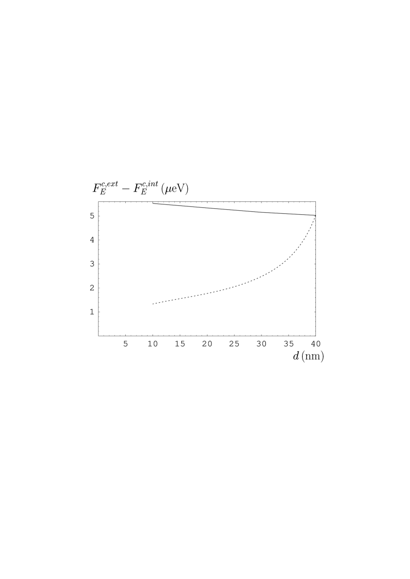
Figure 8: Difference of the free energies of hydrogen atoms situated outside and inside of the multiwall carbon nanotube as a function of nanotube thickness. The solid and dashed lines are for the nanotubes with a fixed internal radius $R_{0}=10\,$nm and fixed external radius $R=50\,$nm, respectively.

Now we are in a position to compare the free energies of hydrogen atoms located outside and inside a multiwall carbon nanotube in order to decide which position is preferable energetically. In Fig. 8 the calculation results for the differences of free energies $F_{E}^{c,ext}$ and $F_{E}^{c,int}$ are presented as a function of thickness of the nanotube. In doing so we consider both atoms, internal and external, situated at a separation $a=3\,$nm from the internal and external surfaces of a nanotube, respectively. The solid line in Fig. 8 is related to the fixed internal radius of the nanotube $R_{0}=10\,$nm, and in this case the external radius increases together with thickness of the nanotube $d$. The dashed line is for a fixed external radius $R=50\,$nm and decreasing internal radius with the increase of $d$. The computations were performed with Eq. (43) for a position of the atom inside the nanotube and with Eq. (35) for position of the atom outside the nanotube.

As is seen from Fig. 8, in all cases the difference between the external and internal free energies of the van der Waals interaction is positive. What this means is the position of a hydrogen atom inside a multiwall carbon nanotube is preferable energetically. Comparing the solid and dashed lines in Fig. 8, we conclude that for nanotubes of fixed thickness $d$ the potential well for the hydrogen atom inside a nanotube is deeper if nanotube has a smaller external radius $R$. This is an encouraging result which points to the possibility of hydrogen storage inside carbon nanostructures.

VIII Conclusions and discussion

In the above we have widened the scope of the Lifshitz theory of the van der Waals force by considering new configurations of much interest which have not been explored previously. The first to be investigated was the van der Waals force between an atom or molecule and a plane surface of an uniaxial crystal perpendicular to the crystal optic axis. For this configuration the exact expression for the free energy of the van der Waals and Casimir-Polder interaction is given by Eq. (1) with the reflection coefficients (5) (for the case of a microparticle near a semispace) or (7) (for a microparticle near a plate of finite thickness). We next derive the approximate Lifshitz-type formula (19) for the free energy of the van der Waals interaction between microparticle and solid cylinder or cylindrical shell having a longitudinal concentric cavity. This cylinder may be made of isotropic material or of an uniaxial crystal. The accuracy of the obtained formula was shown to be of about 1% at microparticle-cylinder separations less than one half of a cylinder radius.

The above extensions of the Lifshitz formula for microparticle-wall interaction were applied to the case of hydrogen atom or molecule near a graphite surface. For this purpose the dielectric permittivities of graphite along the imaginary frequency axis were found by the use of tabulated optical data for the complex refractive index. In doing so different sets of data were analyzed and necessary extrapolations to high and low frequencies were done. Together with the use of hydrogen atomic and molecular dynamic polarizabilities, this allowed us to calculate the van der Waals interaction between hydrogen atom or molecule and graphite semispace, graphite flat plate of finite thickness or solid graphite cylinder and cylindrical shell. In particular, the influence of the thickness of the plate on the van der Waals interaction was investigated.

The calculation results for the atom-cylinder case were used to model the van der Waals interaction between hydrogen atoms or molecules and multiwall carbon nanotube with sufficiently large number of layers. In particular, the dependence of the van der Waals interaction of the atom-nanotube case on nanotube thickness was investigated. Notice that the developed formalism is not applicable to single- or twowall nanotubes where the atomic structure of the wall should be taken into account. In this case the van der Waals force can be computed in the framework of density functional theory 39a ; 39b ; 39c .

Finally, we have compared the free energies of the van der Waals interaction between a hydrogen atom and multiwall carbon nanotube for the cases when atom is located outside or inside of the nanotube. It was shown that atoms situated inside of a multiwall nanotube possess lower free energy in a wide region of nanotube thicknesses, i.e., such a position is energetically preferable. This conclusion is promising for the possibility of using carbon nanotubes for the purpose of hydrogen storage.

Many other opportunities for application of the obtained generalizations of the Lifshitz formula in physics of dispersion forces are possible.

Figure 1: Schematic of the cylinder of radius $R$ made of a uniaxial crystal and having a longitudinal concentric cavity of radius $R-d$. This cylinder is concentrically placed into a cylindrical cavity of radius $R+a$ in the infinite space filled with an isotropic substance.

Figure 2: Dielectric permittivity of graphite along the imaginary frequency axis in (a) the hexagonal layer and (b) perpendicular to it, as a function of frequency. Solid and dashed lines in (b) are obtained with the optical data of Ref. 37 and Ref. 36 , respectively.

Figure 3: Dependence of the van der Waals coefficient $C_{3}^{s}$ on separation of (a) hydrogen atom and (b) molecule, from graphite semispace. The solid and dashed lines are obtained with the optical data of Ref. 37 and Ref. 36 , respectively.

Figure 4: The ratios of the free energies for the van der Waals atom-plate to atom-semispace interaction as a function of plate thickness for hydrogen atom located at different separations from the graphite surface (lines 1, 2, 3 and 4 are for separations $a=3\,$nm, $10\,$nm, $20\,$nm and $50\,$nm, respectively).

Figure 5: Dependence of the van der Waals coefficient $C_{3}^{s}$ on the cylinder radius for (a) hydrogen atom and (b) molecule, located at different separations from the graphite cylinder (lines 1, 2 and 3 are for separations $a=3\,$nm, $5\,$nm and $10\,$nm, respectively).

Figure 6: Dependence of the van der Waals coefficient $C_{3}^{s}$ on thickness of the cylindrical shell with an external radius $R=20\,$nm for hydrogen atom at a separation $a=5\,$nm from the shell.

Figure 7: The van der Waals free energy for hydrogen atom inside of the carbon nanotube with internal radius $R_{0}=10\,$nm and external radius $R=50\,$nm as a function of the atom position between the opposite points of the internal cylindrical surface.

Table 1: The values of strengths and eigenenergies of oscillators for hydrogen atom in the framework of the 10-oscillator model.

$j$	$g_{j}$	$\omega_{aj}\,$(a.e.)
1	0.41619993	0.37500006
2	0.08803654	0.44533064
3	0.08993244	0.48877611
4	0.10723836	0.56134416
5	0.10489786	0.68364018
6	0.08700329	0.89169023
7	0.06013601	1.2698693
8	0.03259492	2.0478339
9	0.01199044	4.0423429
10	0.00197021	12.194172

Table 2: Magnitudes of the van der Waals coefficients $C_{3}^{s}$ and $C_{3}^{c}$ and their relative differences $\delta$ (see text) for the interaction of hydrogen atom or molecule with a graphite semispace or a cylinder with radius $R=50\,$nm.

$a$	$H$			$H_{2}$
(nm)	$C_{3}^{s}\,$(a.u.)	$C_{3}^{c}\,$(a.u.)	$\delta$(%)	$C_{3}^{s}\,$(a.u.)	$C_{3}^{c}\,$(a.u.)	$\delta$(%)
3	0.09882	0.09471	4.2	0.1317	0.1262	4.2
5	0.09416	0.08792	6.6	0.1248	0.1166	6.6
10	0.08316	0.07322	12.0	0.1088	0.09584	11.9
20	0.06652	0.05301	20.3	0.08526	0.06801	20.2
30	0.05516	0.04047	26.6	0.06970	0.05118	26.6
40	0.04704	0.03214	31.7	0.05885	0.04025	31.6
50	0.04098	0.02631	35.8	0.05090	0.03270	35.8

References

- (1) J. E. Lennard-Jones, Trans. Faraday Soc. 28, 333 (1932).
- (2) M. Karimi and G. Vidali, Phys. Rev. B 34, 2794 (1986).
- (3) M. Karimi and G. Vidali, Phys. Rev. B 39, 3854 (1989).
- (4) H. B. G. Casimir and D. Polder, Phys. Rev. 73, 360 (1948).
- (5) E. M. Lifshitz and L. P. Pitaevskii, Statistical Physics, Part. II (Pergamon Press, Oxford, 1980).
- (6) F. Shimizu, Phys. Rev. Lett. 86, 987 (2001).
- (7) V. Druzhinina and M. DeKieviet, Phys. Rev. Lett. 91, 193202 (2003).
- (8) R. E. Grisenti, W. Schollkopf, J. P. Toennies, G. C. Hegerfeldt, and T. Kohler, Phys. Rev. Lett. 83, 1755 (1999).
- (9) J. D. Perreault, A. D. Cronin, and T. A. Savas, e-print physics/0312123.
- (10) Y. Lin, I. Teper, C. Chin, and V. Vuletić, Phys. Rev. Lett. 92, 050404 (2004).
- (11) M. Antezza, L. P. Pitaevskii, and S. Stringari, Phys. Rev. A 70, 053619 (2004).
- (12) J. F. Babb, G. L. Klimchitskaya, and V. M. Mostepanenko, Phys. Rev. A 70, 042901 (2004).
- (13) A. O. Caride, G. L. Klimchitskaya, V. M. Mostepanenko, and S. I. Zanette, e-print quant-ph/0503038, Phys. Rev. A, to appear.
- (14) J. Mahanty and B. W. Ninham, Dispersion Forces (Academic Press, London, 1976).
- (15) Yu. S. Barash, van der Waals Forces (Nauka, Moscow, 1988), in Russian.
- (16) J. Blocki, J. Randrup, W. J. Swiatecki, and C. F. Tsang, Ann. Phys. (N.Y.) 105, 427 (1977).
- (17) S. K. Lamoreaux, Phys. Rev. Lett. 78, 5 (1997).
- (18) U. Mohideen and A. Roy, Phys. Rev. Lett. 81, 4549 (1998); G. L. Klimchitskaya, A. Roy, U. Mohideen, and V. M. Mostepanenko, Phys. Rev. A 60, 3487 (1999).
- (19) B. W. Harris, F. Chen, and U. Mohideen, Phys. Rev. A 62, 052109 (2000).
- (20) F. Chen, U. Mohideen, G. L. Klimchitskaya, and V. M. Mostepanenko, Phys. Rev. Lett. 88, 101801 (2002); Phys. Rev. A 66, 032113 (2002).
- (21) R. S. Decca, E. Fischbach, G. L. Klimchitskaya, D. E. Krause, D. López, and V. M. Mostepanenko, Phys. Rev. D 68, 116003 (2003).
- (22) A. C. Dillon, K. M. Jones, T. A. Bekkedahl, C. H. Kiang, D. S. Bethune, and M. J. Heben, Nature 386, 377 (1997).
- (23) R. G. Ding, G. Q. Lu, Z. F. Yan, and M. A. Wilson, J. of Nanoscience and Nanotech. 1, 7 (2001).
- (24) V. Meregalli and M. Parrinello, Appl. Phys. A 72, 143 (2001).
- (25) W. A. Diño, H. Nakanishi, and H. Kasai, e-J. Surf. Sci. Nanotech. 2, 77 (2004).
- (26) I. V. Bondarev and Ph. Lambin, Solid State Commun. 132, 203 (2004).
- (27) I. V. Bondarev and Ph. Lambin, e-print cond-mat/0501593.
- (28) Ch. Girard, Ph. Lambin, A. Dereux, and A. A. Lucas, Phys. Rev. B 49, 11425 (1994).
- (29) F. Zhou and L. Spruch, Phys. Rev. A 52, 297 (1995).
- (30) J. Schwinger, L. L. DeRaad, Jr., and K. A. Milton, Ann. Phys. (N.Y.) 115, 1 (1978).
- (31) P. W. Milonni, The Quantum Vacuum (Academic Press, San Diego, 1994).
- (32) G. L. Klimchitskaya, U. Mohideen, and V. M. Mostepanenko, Phys. Rev. A 61, 062107 (2000).
- (33) M. Bordag, U. Mohideen, and V. M. Mostepanenko, Phys. Rep. 353, 1 (2001).
- (34) D. L. Greenaway, G. Harbeke, F. Bassani, and E. Tosatti, Phys. Rev. 178, 1340 (1969).
- (35) F. D. Mazzitelli, in: Quantum Field Theory Under the Influence of External Conditions, ed. K. A. Milton (Rinton Press, Princeton, 2004).
- (36) F. D. Mazzitelli, M. J. Sancher, N. Scoccola, and J. Von Stecher, Phys. Rev. A 67, 013807 (2003).
- (37) L. D. Landau, E. M. Lifshitz, and L. P. Pitaevskii, Electrodynamics of Continuous Media (Pergamon Press, Oxford, 1984).
- (38) R. E. Johnson, S. T. Epstein, and W. J. Meath, J. Chem. Phys. 47, 1271 (1967).
- (39) S. Rauber, J. R. Klein, M. W. Cole, and L. W. Bruch, Surf. Sci. 123, 173 (1982).
- (40) Handbook of Optical Constants of Solids, ed. E. D. Palik (Academic, New York, 1991) pp.449–460.
- (41) R. Klucker, M. Skilowski, and W. Steinmann, Phys. Stat. Sol. (b) 65, 703 (1974).
- (42) H. Venghaus, Phys. Stat. Sol. (b) 71, 609 (1975).
- (43) L. G. Johnson and G. Dresselhaus, Phys. Rev. B 7, 2275 (1973).
- (44) V. M. Mostepanenko and N. N. Trunov, The Casimir Effect and its Applications (Clarendon Press, Oxford, 1997).
- (45) A. Bogicevic, S. Ovesson, P. Hyldgaard, B. I. Lundqvist, H. Brune, and D. R. Jennison, Phys. Rev. Lett. 85, 1910 (2000).
- (46) E. Hult, P. Hyldgaard, and B. I. Lundqvist, Phys. Rev. B 64, 195414 (2001).
- (47) H. Rydberg, M. Dion, N. Jacobson, E. Schröder, P. Hyldgaard, S. I. Simak, D. C. Landreth, and B. I. Lundqvist, Phys. Rev. Lett. 91, 126402 (2003).