Detection of atomic entanglement and electromagnetically induced transparency in velocity-selective coherent population trapping

Abstract

We investigate theoretically the optical properties of an atomic gas which has been cooled by the laser cooling method velocity-selective coherent population trapping. We demonstrate that the application of a weak laser pulse gives rise to a backscattered pulse, which is a direct signal for the entanglement in the atomic system, and which leads to single-particle entanglement on the few-photon level. If the pulse is applied together with the pump lasers, it also displays the phenomenon of electromagnetically induced transparency. We suggest that the effect should be observable in a gas of Rubidium atoms.

I Introduction

Among a large variety of laser cooling schemes that have been developed, velocity-selective coherent population trapping (VSCPT) belongs to a small group of methods by which temperatures below the one-photon recoil energy can be achieved. One-dimensional realizations of the VSCPT-method have been demonstrated for ⁴He vscptexp1 and ⁸⁷Rb atoms haensch . In addition, VSCPT experiments with Helium atoms have been carried out successfully in two vscptexp2 and three vscptexp3 dimensions.

The fundamental feature on which VSCPT relies is the preparation of an atomic dark state (see, e.g., Ref. stirap ) which does not couple to the pump lasers. However, there is a significant difference between conventional dark states and the state of a VSCPT gas: In the former case it is preferable to consider situations in which the atomic center-of-mass motion can be neglected. This is for example the case if all laser fields are propagating in one direction, the corresponding dark state is then simply a superposition of two hyperfine ground states. By contrast, the dark state of a VSCPT gas must depend on the center-of-mass motion to achieve the desired cooling effect. Therefore, the atoms are exposed to two counter-propagating pump lasers with wavenumber $k_{p}$. The dark state of this laser configuration

$$|\,\text{VSCPT}\,\rangle:=\frac{1}{\sqrt{2}}\big{[}\,|\,-\,\rangle\otimes|\,-\hbar k_{p}\,\rangle-|\,+\,\rangle\otimes|\,\hbar k_{p}\,\rangle\,\big{]}$$ (1)

is then an entangled superposition of states that contain both internal ($|\,\pm\,\rangle$) and center-of-mass degrees of freedom ($|\,\pm\hbar k_{p}\,\rangle$).

It is this existence of entangled atomic coherences which makes the optical properties of a VSCPT gas interesting. Our goal is to identify a distinctive optical signal which is directly linked to the atomic entanglement. We will show that the latter gives rise to a backscattered beam of light when the VSCPT gas is probed with a weak signal laser pulse (Sec. III). It will be demonstrated that this signal is absent for a mere mixture of ground states and thus would provide a direct test of the entanglement of the atomic system. This effect can also be interpreted as a transfer of entanglement from a single atom to a single photon (Sec. VI). There are two additional features of the VSCPT state which make it a system with very special optical properties. First, since it is prepared in a dark state one can expect that a VSCPT gas also exhibits the phenomenon of electromagnetically induced transparency (EIT) hau1 ; fleischhauer1 ; phillips1 ; this will be examined in Sec. V. We remark here that EIT in a standing-wave geometry has also been studied by Affolderbach et al. affolderbach . Although the laser configuration is similar to that considered here, the physical system is quite different since the experiments are conducted at room temperature. A second feature of the VSCPT state is that it is a periodic state of matter in position space ($\langle z|\,\text{VSCPT}\,\rangle\propto\exp(\pm ipz/\hbar)$). While one may conjecture that this would cause the creation of band gaps in the photonic spectrum it will become clear in our derivations that this is not the case.

II Theory of the VSCPT state

Our aim is to find an optical signature for the entanglement between the atomic internal and center-of-mass degrees of freedom in a VSCPT state, as well as to explore its potential for EIT effects. To do so we first describe the features of an atomic VSCPT state, which has been experimentally realized with ⁴He vscptexp1 as well as ⁸⁷Rb atoms haensch . The atoms are exposed to two counter-propagating pump laser beams which share the same frequency $\omega_{p}$ and Rabi frequency $\Omega_{p}$. The electronic degrees of freedom of the atoms are modeled by a three-level system in $\Lambda$-configuration (see Fig. 1). In addition, the atomic center-of-mass motion is treated quantum mechanically. In the one-dimensional cooling scheme considered here the momentum components perpendicular to the pump field are not observed and can therefore be traced out. The atomic Hamiltonian is then given by

$$H_{0}:=\frac{\hat{p}_{z}^{2}}{2\,m}\,+\,\hbar\,\omega_{0}\,|\,e\,\rangle\langle\,e\,|\;,$$ (2)

where $m$ is the mass of the atom and $\omega_{0}$ its resonance frequency. In the rotating wave approximation the interaction Hamiltonian takes the form

$$H_{p} := -\,\left(\,|\,e\,\rangle\langle\,-\,|\,e^{ik_{p}\hat{z}}\hskip 34.14322pt\right.$$

$$\qquad\quad\left.+\,|\,e\,\rangle\langle\,+\,|\,e^{-ik_{p}\hat{z}}\,\right)\,e^{-i\omega_{p}t}\,\hbar\,\Omega_{p}\,+\,\text{H.c.}\;,$$

where $\Omega_{p}:=dE_{p}/\hbar$ is the Rabi frequency of the pump lasers ($d:=\langle\,e\,|\mbox{\boldmath$\hat{d}$\unboldmath}\cdot\mbox{\boldmath$\epsilon$\unboldmath}^{(\pm)}|\,\mp\,\rangle$ and $\hat{d}$ is the electric-dipole moment operator). $E_{p}$ denotes the electric-field amplitude of the classical pump field $\mbox{\boldmath$E$\unboldmath}_{p}(z,t)=\mbox{\boldmath$E$\unboldmath}_{p}^{(+)}(z,t)+\mbox{\boldmath$E$\unboldmath}_{p}^{(-)}(z,t)$, with

$$\mbox{\boldmath$E$\unboldmath}_{p}^{(+)}(z,t) := E_{p}e^{-i\omega_{p}t}\left(\mbox{\boldmath$\epsilon$\unboldmath}^{(+)}e^{ik_{p}z}+\mbox{\boldmath$\epsilon$\unboldmath}^{(-)}e^{-ik_{p}z}\right)$$ (4)

being the positive-frequency part of the electric field and $\mbox{\boldmath$E$\unboldmath}_{p}^{(-)}=\mbox{\boldmath$E$\unboldmath}_{p}^{(+)\dagger}$. The circular polarization vectors are defined as $\mbox{\boldmath$\epsilon$\unboldmath}^{(\pm)}:=\left(\mbox{\boldmath$e$\unboldmath}_{x}\pm i\mbox{\boldmath$e$\unboldmath}_{y}\right)/\sqrt{2}$ .

Figure 1: $\Lambda$-type pumping scheme including translational degrees of freedom. A $\sigma^{+}$ polarized beam travels along the positive $z$-direction and couples the ground state $|-,p-\hbar k_{p}\rangle$ to the excited state $|e,p\rangle$. The counter-propagating beam is $\sigma^{-}$ polarized and couples the ground state $|+,p+\hbar k_{p}\rangle$ to the excited state.

The special linear combination of ground states

$$|\,D(p)\,\rangle:=\frac{1}{\sqrt{2}}\,\big{[}\,|\,-,p-\hbar k_{p}\,\rangle\,-\,|\,+,p+\hbar k_{p}\,\rangle\,\big{]}$$ (5)

is an eigenstate of the interaction Hamiltonian $H_{p}$ and therefore decoupled from the light field. However, $|\,D(p)\,\rangle$ is generally not an eigenstate of $H_{0}$. Only for $p=0$ the state $|\,\mbox{\small VSCPT}\,\rangle=|\,D(p=0)\,\rangle$ is an eigenstate of the complete Hamiltonian $H_{\text{C}}(t):=H_{0}+H_{p}(t)$ and therefore stationary.

In principle, a VSCPT state can simply be created by pumping the atoms with laser light. Since spontaneous emission increases the population in $|\text{VSCPT}\rangle$ with a certain probability, and since all other combinations of the ground states can be pumped back to the excited state, the atoms accumulate in $|\text{VSCPT}\rangle$. The corresponding dynamics is governed by the master equation

$$\dot{\varrho}=-\frac{i}{\hbar}\,[H_{\text{C}}(t),\varrho]+\mathcal{L}_{\gamma}\varrho\quad.$$ (6)

The term $\mathcal{L}_{\gamma}\varrho$ on the right hand side accounts for spontaneous emission and is given by vscpttheorie ; spontan ; stenholm

$$\mathcal{L}_{\gamma}\varrho := -\gamma\varrho_{ee}|\,e\,\rangle\langle\,e\,|$$

$$-\frac{\gamma}{2}\,\left[\varrho_{e-}|\,e\,\rangle\langle\,-\,|\,+\,\varrho_{e+}|\,e\,\rangle\langle\,+\,|\,+\,\text{H.c.}\right]$$

$$\hskip 19.91684pt+\,\frac{\gamma}{2}\int\limits_{-\hbar k_{0}}^{\hbar k_{0}}H(u)\,e^{\frac{i}{\hbar}u\hat{z}}\varrho_{ee}e^{-\frac{i}{\hbar}u\hat{z}}\,\text{d}u\,|\,-\,\rangle\langle\,-\,|$$

$$\hskip 19.91684pt+\,\frac{\gamma}{2}\int\limits_{-\hbar k_{0}}^{\hbar k_{0}}H(u)\,e^{\frac{i}{\hbar}u\hat{z}}\varrho_{ee}e^{-\frac{i}{\hbar}u\hat{z}}\,\text{d}u\,|\,+\,\rangle\langle\,+\,|$$

with $\varrho_{\epsilon\epsilon^{\prime}}:=\langle\,\epsilon\,|\varrho|\,\epsilon^{\prime}\,\rangle\quad(\epsilon,\,\epsilon^{\prime}\,\in\,\{e,\,-,\,+\})$. For the $J_{e}=1\leftrightarrow J_{g}=1$ transition considered here, the function $H(u)$ is given by $H(u):=3\,\,(1+u^{2}/(\hbar k_{0})^{2})/(8\,\hbar k_{0})$. It has been shown in Ref. vscpttheorie that for a finite duration of the pumping this process results in a finite atomic momentum distribution. We approximate this state by a mixture of dark states with different momenta that is described by the density matrix remark1

$$\varrho_{f}:=\int\limits_{-\infty}^{\infty}f(p)\,|\,D(p)\,\rangle\langle\,D(p)\,|\,\text{d}p\;,$$ (8)

where $f$ characterizes the momentum distribution. We assume here that $f$ can be approximated by a Gaussian distribution centered around $p=0$,

$$f(p)=\frac{1}{\sqrt{2\pi}\,\sigma_{p}}\,e^{-p^{2}/(2\sigma_{p}^{2})}\;.$$ (9)

The momentum width is given by $\sigma_{p}^{2}=\int p^{2}f(p)\text{d}p$. It is a measure of the achieved final temperature of the gas and varies with the coherent interaction time $\Theta$ as $\sigma_{p}\sim 1/\sqrt{\Theta}$. The experiments presented in Refs. vscptexp1 ; haensch demonstrate that a value of $\sigma_{p}\approx\hbar k_{p}/2$ is achievable.

III Coherent backscattering of a weak signal beam

The optical response of an atomic gas can be described by the Maxwell-Bloch equations, which include an atomic master equation of the form (6) and the wave equation for the electric field,

$$\left(\frac{1}{c^{2}}\,\partial_{t}^{2}\,-\,\Delta\right)\mbox{\boldmath$E$\unboldmath}=-\frac{1}{c^{2}\,\varepsilon_{0}}\,\ddot{\mbox{\boldmath$P$\unboldmath}}\;.$$ (10)

For a dilute gas, atom-atom interactions can be neglected so that the macroscopic polarization $P$ can be expressed as the local mean value of the single-atom dipole operator,

$$\mbox{\boldmath$P$\unboldmath}(z,t):=\bar{\rho}\,\mbox{Tr}_{\text{int}}\big{(}\varrho(z,t)\mbox{\boldmath$\hat{d}$\unboldmath}\big{)}\;.$$ (11)

Here, $\bar{\rho}$ denotes the mean atomic density and the trace runs over the internal states ($\varrho(z,t)=\langle\,z\,|\varrho(t)|\,z\,\rangle$).

Figure 2: Idealized set-up after the pump laser beams have been switched off. The VSCPT gas stretches from $z=0$ to $z=a$ (region II) and is surrounded by vacuum (region I and III). The signal beam, a plane-wave with frequency $\omega_{s}$, $\sigma^{+}$ polarization and amplitude $E_{0}$ is shone into the probe from the left.

To investigate the optical properties of a gas that has been cooled by means of the VSCPT method, we generally consider the behavior of a weak signal laser beam interacting with a homogeneous distribution of cooled atoms of finite width $a$. In this section we examine the case where the signal beam is switched on after the pump lasers are switched off. We will see in Sec. V that the optical response will be quite different when the pump lasers are not switched off.

The setup to investigate the optical response is shown in Fig. 2. At time $t=0$, the pump field is turned off and a $\sigma^{+}$ polarized signal field

$$\mbox{\boldmath$E$\unboldmath}_{1}^{(+)}(z,t)=E_{1}(z)\mbox{\boldmath$\epsilon$\unboldmath}^{(+)}e^{i(k_{s}z-\omega_{s}t)}$$ (12)

with slowly varying amplitude $E_{1}(z)$ and frequency $\omega_{s}$ is applied to the probe from the left. The associated atomic evolution can be derived from Eq. (6) with $H_{\text{C}}$ replaced by $H_{0}+H_{\text{s}}(t)$, with

$$H_{\text{s}}(t) = -\hbar\Omega_{1}\,e^{ik_{s}\hat{z}}\,e^{-i\omega_{s}t}|e\rangle\langle-|$$ (13)

$$-\hbar\Omega_{2}\,e^{ik_{2}\hat{z}}\,e^{-i\omega_{s}t}|e\rangle\langle+|\;+\;\text{H.c.}$$

and $\Omega_{i}:=d\,E_{i}(z)/\hbar$. The second electric field

$$\mbox{\boldmath$E$\unboldmath}_{2}^{(+)}(z,t):=E_{2}(z)\,\mbox{\boldmath$\epsilon$\unboldmath}^{(-)}e^{i(k_{2}z-\omega_{s}t)}$$ (14)

($k_{2}:=k_{s}-2k_{p}\approx-k_{s}$) has been introduced to keep the ansatz consistent (see below). To solve the Maxwell-Bloch equations we first consider the atomic master equation. Since the signal beam is assumed to be weak, its influence on the atoms can be treated in first-order perturbation theory. Expanding the density matrix as $\varrho=\varrho_{0}+\varrho_{1}$ we then find

$$\dot{\varrho}_{0} = \mathcal{L}_{0}\varrho_{0}$$ (15)

$$\big{[}\partial_{t}\,-\,\mathcal{L}_{0}\big{]}\varrho_{1} = -\frac{i}{\hbar}\left[H_{\text{s}},\varrho_{0}\right]\;.$$ (16)

The Liouville operator $\mathcal{L}_{0}$ is defined as

$$\mathcal{L}_{0}(\,\cdot\,):=-\frac{i}{\hbar}\,[H_{0},\,\cdot\,]\,+\,\mathcal{L}_{\gamma}(\,\cdot\,)$$ (17)

and governs the time evolution of the free atom.

We first consider the ideal case where $\varrho_{0}$ is given by the stationary state $\varrho_{\text{s}}\equiv|\text{VSCPT}\rangle\langle\text{VSCPT}|$. For brevity we will only discuss the incoming signal beam $\mbox{\boldmath$E$\unboldmath}_{1}$ since the second beam can be treated in an analogous way linearity . The commutator on the right hand side of eq. (16) is comprised of two time-dependent parts

$$-\,\frac{i}{\hbar}\left[H_{\text{s}},\varrho_{\text{s}}\right]=\frac{i\Omega_{1}}{\sqrt{2}}|e,\hbar\Delta k\rangle\langle\text{VSCPT}|e^{-i\omega_{s}t}\,+\,\text{H.c.}$$ (18)

that vary with $e^{-i\omega_{s}t}$ and $e^{i\omega_{s}t}$, respectively ($\Delta k:=k_{s}-k_{p}$). This inhomogeneity gives rise to the following steady-state solution

$$\varrho_{1}(t) = -\,\frac{1}{2}\,\chi_{0}(\omega_{s})\,\Omega_{1}\,e^{-i\omega_{s}t}\,|\,e,\hbar\Delta k\,\rangle\langle\,-,-\hbar k_{p}\,|$$

$$+\,\frac{1}{2}\,\chi_{0}(\omega_{s})\,\Omega_{1}\,e^{-i\omega_{s}t}\,|\,e,\hbar\Delta k\,\rangle\langle\,+,\hbar k_{p}\,|\,+\,\mbox{H.c.}$$

with

$$\chi_{0}(\omega_{s}):=\left[\,\left(E_{r}-\frac{\hbar{\Delta k}^{2}}{2m}\right)+i\,\frac{\gamma}{2}+\Delta_{s}\,\right]^{-1}\quad.$$ (20)

$E_{r}:=\hbar k_{p}^{2}/(2m)$ defines the recoil frequency and $\Delta_{s}:=\omega_{s}-\omega_{0}$ denotes the detuning of the signal field from resonance. In the following we will use this steady-state solution instead of a full solution that fulfills the correct initial condition $\varrho_{1}(t)=0$. This is justified if the interaction time between the laser (pulses) and the atoms is long compared to the natural lifetime of the excited state, since in this case all non-stationary contributions (which are solutions of the homogeneous equations) are damped away.

We remark that, as a consequence of first-order perturbation theory, the population of the excited state remains zero. This explains the simple form of solution (III) and effectively allows us to replace the full decoherence term (II) by

$$\mathcal{L}_{\gamma}^{\text{\small coh}}\varrho:=-\frac{\gamma}{2}\,\left[\varrho_{e-}|\,e\,\rangle\langle\,-\,|+\varrho_{e+}|\,e\,\rangle\langle\,+\,|+\mbox{H.c.}\right]\;.$$

An important feature of Eq. (III) is the non-vanishing coherence $[\varrho_{1}]_{e+}:=\langle\,e\,|\varrho_{1}|\,+\,\rangle$. This effect does not appear if the state $\varrho_{0}=|\text{VSCPT}\rangle\langle\text{VSCPT}|$ is replaced by an incoherent mixture of the form

$$\varrho_{\text{mix}}:=\frac{1}{2}\big{[}|\,-,-\hbar k_{p}\,\rangle\langle\,-,-\hbar k_{p}\,|+|\,+,\hbar k_{p}\,\rangle\langle\,+,\hbar k_{p}\,|\big{]}\;,$$

and therefore is a signal for the coherence between the atomic ground states.

We will now show that this coherence creates a backscattered light beam and therefore generates a signal of the entanglement between atomic internal and center-of-mass degrees of freedom. To do this we solve the wave equation (10) in paraxial approximation, i.e., we neglect the terms $\partial_{z}^{2}E_{i}(z)$ ($i\in\{1,2\}$). This is justified if the envelopes $E_{i}(z)$ are slowly varying over one wavelength, so that

$$\left|\partial_{z}^{2}E_{i}(z)\right|\ll k_{s}\,\left|\partial_{z}E_{i}(z)\right|\;.$$ (21)

Inserting $\varrho_{1}$ of Eq. (III) and the corresponding contribution induced by $\mbox{\boldmath$E$\unboldmath}_{2}$ into Eq. (11) leads to

$$\mbox{\boldmath$P$\unboldmath}^{(+)}(z,t) = \frac{\bar{\rho}d^{*}}{2}\chi_{0}(\omega_{s})\left(\big{(}\Omega_{2}-\Omega_{1}\big{)}e^{ik_{s}z}\mbox{\boldmath$\epsilon$\unboldmath}^{(+)}\right.$$

$$\hskip 22.76228pt\left.+\big{(}\Omega_{1}-\Omega_{2}\big{)}e^{ik_{2}z}\mbox{\boldmath$\epsilon$\unboldmath}^{(-)}\right)e^{-i\omega_{s}t}\;.$$

The term $\sim\Omega_{1}\mbox{\boldmath$\epsilon$\unboldmath}^{(-)}$ is a direct consequence of $[\varrho_{1}]_{e+}\neq 0$. In the paraxial wave equation neglect ,

$$k_{s}\partial_{z}E_{1}(z)\mbox{\boldmath$\epsilon$\unboldmath}^{(+)}e^{ik_{s}z}\hskip 68.28644pt$$ (23)

$$-\,k_{s}\big{(}\partial_{z}E_{2}(z)+2i\Delta kE_{2}(z)\big{)}\mbox{\boldmath$\epsilon$\unboldmath}^{(-)}e^{ik_{2}z} = \frac{e^{i\omega_{s}t}}{2ic^{2}\,\varepsilon_{0}}\,\ddot{\mbox{\boldmath$P$\unboldmath}}^{(+)}\;,$$

this results in a coupling between $E_{1}$ and $E_{2}$. If $E_{2}$ had not been introduced, the term $\sim\Omega_{1}\mbox{\boldmath$\epsilon$\unboldmath}^{(-)}$ would not have a corresponding term $\sim\mbox{\boldmath$\epsilon$\unboldmath}^{(-)}$ on the left-hand side, so that the equation would be inconsistent. Sorting the terms according to their polarization and phase factors leads to a coupled equation for the amplitudes,

$$\partial_{z}\left(\begin{array}[]{c}E_{1}\\ E_{2}\end{array}\right)=\left(\begin{array}[]{cc}-in_{0}&in_{0}\\ -in_{0}&i(n_{0}-2\,\Delta k)\end{array}\right)\left(\begin{array}[]{c}E_{1}\\ E_{2}\end{array}\right)\;,$$ (24)

where

$$n_{0}(\omega_{s}):=\frac{1}{2\,k_{s}}\,\frac{\omega_{s}^{2}\,\bar{\rho}\,|d|^{2}}{2c^{2}\varepsilon_{0}\hbar}\,\chi_{0}(\omega_{s})\quad.$$ (25)

Figure 3: Intensity of the incoming (solid line) and the reflected (dashed line) beam in a VSCPT-gas of length $a=1\,$cm. Both intensities are related to the intensity $I_{0}$ of the incoming beam in region I (Fig. 2).

The boundary conditions on the physical solution are determined by the behavior of $E_{1}$ and $E_{2}$ outside the gas and Maxwell’s equation $\nabla\times\mbox{\boldmath$E$\unboldmath}=-\dot{\mbox{\boldmath$B$\unboldmath}}$, which implies that the transverse electric field is continous at the boundary of the gas (see Fig. 2). Since $E_{1}$ corresponds to the incoming signal beam that travels along the positive $z$-axis, its amplitude is given by a fixed value $E_{1}(z)=E_{0}$ for $z<0$ (region I). On the other hand, the counter-propagating field $E_{2}$ is initially empty so that $E_{2}(z)=0$ for $z>a$ (region III). The boundary conditions for the amplitudes $E_{1,2}$ in region II are thus given by boundary

$$E_{1}(z=0)\stackrel{{\scriptstyle!}}{{=}}E_{0}\quad\text{and}\quad E_{2}(z=a)\stackrel{{\scriptstyle!}}{{=}}0\;.$$ (26)

Introducing the notation $\delta:=\sqrt{(2n_{0}-\Delta k)\Delta k}$ the full solution of Eq. (24) is found to be

$$E_{1}(z) =$$

$$E_{0}\,\frac{\delta\cosh[\delta(a-z)]+i(n_{0}-\Delta k)\sinh[\delta(a-z)]}{\delta\cosh[\delta a]+i(n_{0}-\Delta k)\sinh[\delta a]}e^{-i\Delta kz}$$

$$E_{2}(z) = E_{0}\,\frac{i\,n_{0}\sinh[\delta(a-z)]}{\delta\cosh[\delta a]+i(n_{0}-\Delta k)\sinh[\delta a]}e^{-i\Delta kz}\;.$$

The envelopes $E_{1,2}$ contain a periodic part whose period $\lambda$ is given by the inverse imaginary part of $\delta$. For atomic densities lower than $10^{12}\text{cm}^{-3}$ the parameter $\lambda$ is usually orders of magnitudes larger than the typical length of a VSCPT gas (i.e., a few centimeters); the periodicity would then not be observable. Generally, for $|a\delta|\ll 1$ and $\Delta k\rightarrow 0$ Eq. (III) simplifies considerably and becomes

$$E_{1}(z) = E_{0}\,\left(1-\frac{n_{0}z}{n_{0}a-i}\right)$$ (28)

$$E_{2}(z) = E_{0}\,\left(\frac{n_{0}(a-z)}{n_{0}a-i}\right)\;,$$

which is an excellent approximation for realistic parameters.

Fig. 3 shows a plot of the intensity of the incoming and reflected beam. We chose a probe length of $a=1\,$cm and a detuning of $\Delta_{s}=3\times 10^{6}\,s^{-1}$. For the $J_{e}=1\,\leftrightarrow\,J_{g}=1$ transition of the $D_{1}$ Line of ⁸⁷Rb, the recoil frequency, the rate of spontaneous emission and the dipole moment take the values rb $E_{r}=2.3\times 10^{4}\,s^{-1}$, $\gamma=3.61\times 10^{7}\,s^{-1}$ and $d=2.99\,e\,a_{0}/\sqrt{12}$, where $e$ is the elementary charge and $a_{0}$ is Bohr’s radius. In addition, we assumed a mean atomic density $\bar{\rho}$ of $2\times 10^{10}\,\text{cm}^{-3}$ which is close to the experimental conditions ($\bar{\rho}\approx 10^{10}\,\text{cm}^{-3}$) described in Ref. haensch . About 30% of the incoming intensity is transferred to the reflected beam, all losses are due to spontaneous emission.

Simplified explanation of the backscattered beam: Since the above derivation is somewhat involved we will give here another, more physical explanation of the effect. The incoming signal beam transfers the initial atomic state $|\,\text{VSCPT}\,\rangle$ to the superposition $|\psi_{1}\rangle\sim|\,\text{VSCPT}\,\rangle+H_{s}|\,\text{VSCPT}\,\rangle\sim|\,\text{VSCPT}\,\rangle+|e,p=0\rangle$ (for simplicity we here set $\Delta k=k_{s}-k_{p}$ to zero). Hence, the absorption of an incoming signal photon leads to a (partial) transfer of the initial coherence between $|-,-\hbar k_{p}\rangle$ and $|+,\hbar k_{p}\rangle$ to one between $|e,0\rangle$ and $|+,\hbar k_{p}\rangle$. The latter corresponds to an induced dipole moment which, due to angular momentum conservation, can only lead to emission of photons with polarisation $\sigma^{-}$. In Maxwell’s equations such photons are coupled to the coherence $\rho_{e+}(z,z)=\langle e,z|\psi_{1}\rangle\langle\psi_{1}|+,z\rangle$ at the position z of the atom. An elementary calculation leads to $\rho_{e+}(z,z)$ $\sim\langle e,z\nobreak{|e,0\rangle}\langle+,\hbar k_{p}|+,z\rangle\sim\exp(-ik_{p}z)$ so that the emitted photons are propagating in the opposite direction of the incoming beam. The associated change in the photon’s momentum is provided by the different atomic momenta in the two ground states. The $\sigma^{-}$ polarized backscattered light beam $\mbox{\boldmath$E$\unboldmath}_{2}$ is thus not only a signal for the coherence of the VSCPT state, but also a direct signal of the entanglement between atomic internal and center-of-mass degrees of freedom.

This method of probing entanglement in atomic gases should not only be applicable to a VSCPT gas but to any state in which an entanglement between internal states and momentum states is achieved. The VSCPT gas is only special in that the entangled state is also a dark state with respect to the pump laser field. We will see below that this will lead to EIT for the pair of signal fields. We also emphasize that a mere mixture of states with different momentum and internal degrees of freedom, as it is created by other cooling methods such as Raman cooling raman92 , would not display the backscattered beam.

IV Finite momentum width: dephasing of the reflected beam

In reality the atoms are not prepared in the ideal state $|\text{VSCPT}\rangle\langle\text{VSCPT}|$ but have a finite momentum width, described by $\varrho_{f}$ of Eq. (8). Since this is not a stationary state, the free time evolution of the unperturbed density operator $\varrho_{0}$ of Eq. (15) after the pump lasers are switched off reads

$$\varrho_{0}(t)\,=\int_{-\infty}^{\infty}f(p)\,|\,D(p,t)\,\rangle\langle\,D(p,t)\,|\,\text{d}p\;,$$ (29)

where

$$|\,D(p,t)\,\rangle=\frac{|-,p-\hbar k_{p}\rangle}{\sqrt{2}}-e^{-i\omega_{r}(p)t}\frac{|+,p+\hbar k_{p}\rangle}{\sqrt{2}}$$ (30)

and $\omega_{r}(p):=2k_{p}p/m$. The energy $\hbar\omega_{r}(p)$ is just the difference between the kinetic energies of the ground states $|\,-,p-\hbar k_{p}\,\rangle$ and $|\,+,p+\hbar k_{p}\,\rangle$.

$\varrho_{0}(t)$ describes a mixture of initially dark states which evolve into a corresponding bright state at rates which depend linearly on $p$. To demonstrate that this behavior results in a dephasing of the backscattered wave we proceed as in section III to derive the macroscopic polarization (we only write down the part induced by $\mbox{\boldmath$E$\unboldmath}_{1}$)

$$\mbox{\boldmath$P$\unboldmath}^{(+)}(z,t)=-\frac{\bar{\rho}d^{*}}{2}\Omega_{1}\Big{(}I_{\alpha}\,e^{ik_{s}z}\,\mbox{\boldmath$\epsilon$\unboldmath}^{(+)}-I_{\beta}e^{-ik_{s}z}\mbox{\boldmath$\epsilon$\unboldmath}^{(-)}\Big{)}e^{-i\omega_{s}t}$$ (31)

with

$$I_{\alpha} := \int\limits_{-\infty}^{\infty}\chi(\omega_{s},p)f(p)\text{d}p\;,$$

$$I_{\beta} := \int\limits_{-\infty}^{\infty}\chi(\omega_{s},p)f(p)e^{i\omega_{r}(p)t}\text{d}p$$

$$\chi(\omega_{s},p) := \left[E_{r}+i\frac{\gamma}{2}+\Delta_{s}-\frac{1}{2}\omega_{r}(p)\right]^{-1}\;.$$

In the derivation we have used the approximations $E_{r}-\hbar\Delta k^{2}/(2m)\approx E_{r}$ and $k_{p}\pm\Delta k\approx k_{p}$ as well as $k_{2}\approx-k_{s}$. The evaluation of the integrals $I_{\alpha}$ and $I_{\beta}$ can be simplified by using that $\chi(\omega_{s},p)$ as a function of $p$ is almost constant over the momentum range of a VSCPT gas. We assume here that the momentum width is given by $\sigma_{p}=\hbar k_{p}/2$ (see Sec. II) and are thus allowed to replace $\chi(\omega_{s},p)$ by $\chi_{0}(\omega_{s})$, which yields

$$I_{\alpha}\approx\chi_{0}(\omega_{s})\quad,\quad I_{\beta}\approx\chi_{0}(\omega_{s})\,g\;,$$ (32)

with $g(t):=e^{-2\,E_{r}^{2}\,t^{2}}$.

These results enable us to describe the long-term behavior of the system. For $t\gg 1/E_{r}$, the Integral $I_{\beta}$ is approximately zero and the term proportional to $\mbox{\boldmath$\epsilon$\unboldmath}^{(-)}$ in eq. (31) can be neglected. Consequently, the backscattered wave is equal to zero. The reason is that the dephasing of the coherences in different dark states $|D(p,t)\rangle$ of (30) leads to a destructive interference between the backscattered signal beams for different momenta.

Although the backscattered signal is suppressed for continuously operating signal beams, it is reasonable to expect that it will be strong enough if one employs signal pulses instead. Incoming and backscattered pulses can formally be described by assuming that the amplitudes $E_{1,2}$ of Eqs. (12) and (14) are slowly varying both in space and in time,

$$\left|\partial_{z}^{2}E_{1,2}(z,t)\right| \ll k_{s}\,\left|\partial_{z}E_{1,2}(z,t)\right|\;,$$

$$\left|\partial_{t}^{2}E_{1,2}(z,t)\right| \ll \omega_{s}\,\left|\partial_{t}E_{1,2}(z,t)\right|\ll\omega_{s}^{2}\,\left|E_{1,2}(z,t)\right|\;.$$

Maxwell’s equation (10) becomes now a coupled set of first-order partial differential equations vgroup for the envelopes $E_{1}$ and $E_{2}$,

$$\left(\frac{1}{c}\,\partial_{t}\,+\,\partial_{z}\right)E_{1} = in_{0}\,\big{(}E_{2}\,g-E_{1}\big{)}$$ (33)

$$\left(\frac{1}{c}\,\partial_{t}\,-\,\partial_{z}\right)E_{2} = in_{0}\,\big{(}E_{1}\,g-E_{2}\big{)}\quad,$$

where $n_{0}$ is defined in Eq. (25).

We have numerically solved these equations for a Gaussian amplitude $E_{1}$ incoming from the left, with the boundary condition that $E_{2}$ is zero on the right-hand side of the medium, and that the fields are continuous at the boundary of the medium. At $t=0$, the $E_{1}$ pulse is completely outside of the medium and $E_{2}$ is zero everywhere. The numerical solution is easily obtained using standard mathematical software packages such as Mathematica. The results can be summarized as follows.

The time dependence of $\varrho_{0}$ manifests itself solely in the presence of the function $g$. For a signal pulse whose length is short enough so that $g\approx 1$, the efficiency of the backscattering-effect is as high as for the idealized VSCPT-gas (Sec. III). Fig. 4 shows a plot of $g$ as a function of time for the Helium and Rubidium parameters.

Figure 4: Plot of $g(t)=\exp[-2\,E_{r}^{2}\,t^{2}]$ as a function of time. The recoil frequency of ⁸⁷Rb ($E_{r}=2.3\times 10^{4}\,s^{-1}$) is about 10 times smaller than for ⁴He ($E_{r}=2.7\times 10^{5}\,s^{-1}$).

The small mass of ⁴He results in a large recoil frequency ($E_{r}=2.7\times 10^{5}s^{-1}$) and causes a rapid decay of $g$ within $5\,\mu s$. Consequently, the length of the incoming pulse must be as short as $2\times 10^{-7}\,s$ in order to maximize the peak intensity of the backscattered pulse. However, one should bear in mind that the solution to the homogenous part of eq. (16) cannot be neglected for $t\leq 1/\gamma$. Therefore, the predictions of our theory are only correct for pulses of a few $\mu s$ or longer. In the case of Helium, the efficiency of the backscattering-effect is less than 1% if a Gaussian pulse of $2\,\mu s$ is shone into the probe.

A completely different behavior should be observed for a VSCPT gas of Rubidium atoms. The recoil frequency of Rubidium is about ten times smaller than for Helium, and $g$ is almost constant within the first $5\,\mu s$. Even for a Gaussian pulse of $4\,\mu s$, the peak intensity of the backscattered signal beam is almost as high as in the case of the idealized VSCPT gas (section III). Thus, we expect that for signal pulses traveling through a Rubidium gas the backscattered beam should be a good signal for the entanglement between the electronic and center-of-mass degrees-of-freedom in a VSCPT state.

V Electromagnetically induced transparency

We will now demonstrate that a VSCPT-gas creates electromagnetically induced transparency hau1 ; hau2 ; fleischhauer1 ; fleischhauer2 ; scully ; phillips1 if the signal and the pump field interact with the gas at the same time. In presence of the pump field, the Hamiltonian in Eq. (6) has to be replaced by $H_{\text{C}}+H_{\text{s}}$. The same perturbative methods that have been employed in section III can be applied here, provided the signal field is much weaker than the pump field ($|\Omega_{s}|/|\Omega_{p}|\ll 1$). We consider the simplified situation where all atoms are initially in the unperturbed stationary state $|\text{VSCPT}\rangle$; the previous section indicates that this is justified for sufficiently short signal pulses. The first order correction $\varrho_{1}$ is now determined by

$$\big{[}\partial_{t}-\mathcal{L}_{\text{C}}\big{]}\varrho_{1}=-\frac{i}{\hbar}\left[H_{\text{s}},\varrho_{0}\right]\;,$$ (34)

where $\mathcal{L}_{\text{C}}$ is defined as

$$\mathcal{L}_{\text{C}}(\,\cdot\,):=-\frac{i}{\hbar}\,[H_{\text{C}},\,\cdot\,]\,+\,\mathcal{L}_{\gamma}(\,\cdot\,)$$

with $H_{\text{C}}=H_{0}+H_{p}$. The unitary transformation

$$U:=|\,e\,\rangle\langle\,e\,|e^{i\omega_{p}t}+|\,-\,\rangle\langle\,-\,|e^{ik_{p}\hat{z}}+|\,+\,\rangle\langle\,+\,|e^{-ik_{p}\hat{z}}$$

removes the operators $\exp[\pm ik_{s}\hat{z}]$ as well as the time dependence from the interaction Hamiltonian $H_{p}$. The transformed operator $\tilde{\varrho_{1}}:=U\varrho_{1}U^{\dagger}$ then obeys a more convenient equation than Eq. (34). The remaining calculation follows exactly the procedure of Sec. III. In particular, the matrix element $\langle\,e\,|\varrho_{1}|\,e\,\rangle$ vanishes even in the presence of the pump field. This is a consequence of the initial atomic state $|\text{VSCPT}\rangle$ being an eigenstate of the complete Hamiltonian $H_{\text{C}}$. If the finite width of the atomic momentum distribution is taken into account, excitations will occur and, consequently, side bands of frequency $\omega_{\text{sb}}:=\omega_{s}-2\,\Delta\omega$ will be present.

The result for the field amplitudes is again of the form (III) and (28) if one replaces $\delta$, $n_{0}$ and $\chi_{0}$ by $\delta_{p}:=\sqrt{(2n_{p}-\Delta k)\Delta k}$,

$$n_{p}(\omega_{s}):=\frac{1}{2\,k_{s}}\frac{\omega_{s}^{2}\bar{\rho}|d|^{2}}{2c^{2}\varepsilon_{0}\hbar}\chi_{p}(\omega_{s})$$ (35)

and

$$\chi_{p}(\omega_{s}):=\frac{\Delta\omega}{\Delta\omega\left(E_{r}+i\frac{\gamma}{2}+\Delta_{s}\right)-2|\Omega_{p}|^{2}}\;.$$ (36)

We exploited that $\hbar\Delta k^{2}/(2m)$ and $\hbar k_{p}\Delta k/m$ are much smaller than the frequency difference $\Delta\omega:=\omega_{s}-\omega_{p}=c\Delta k$ between the signal and the pump field.

This result allows us to investigate the behavior of a $\sigma^{+}$ polarized signal pulse. The electrical fields $\mbox{\boldmath$E$\unboldmath}_{1}$ and $\mbox{\boldmath$E$\unboldmath}_{2}$ within the medium are then given by

$$\mbox{\boldmath$E$\unboldmath}_{1}^{(+)}(z,t) := \int\limits^{\infty}_{-\infty}\mathcal{E}_{1}\,e^{i\left(\frac{\omega}{c}\,z-\omega\,t\right)}\text{d}\omega\mbox{\boldmath$\epsilon$\unboldmath}^{(+)}$$ (37)

$$\mathcal{E}_{1}(z,\omega) := \frac{1}{\sqrt{2\pi}}\,\mathcal{E}_{0}(\omega)\left(1-\frac{n_{p}(\omega)\,z}{n_{p}(\omega)a-i}\right)$$

and

$$\mbox{\boldmath$E$\unboldmath}_{2}^{(+)}(z,t) := \int\limits^{\infty}_{-\infty}\mathcal{E}_{2}e^{-i\left(\frac{\omega}{c}z+\omega t\right)}\text{d}\omega\mbox{\boldmath$\epsilon$\unboldmath}^{(-)}$$ (38)

$$\mathcal{E}_{2}(z,\omega) := \frac{1}{\sqrt{2\pi}}\,\mathcal{E}_{0}(\omega)\left(\frac{n_{p}(\omega)(a-z)}{n_{p}(\omega)a-i}\right)\quad.$$

At $z=0$, just outside the medium, the electric field $\mbox{\boldmath$E$\unboldmath}_{1}$ reduces to

$$\mbox{\boldmath$E$\unboldmath}_{1}(z=0,t)=E_{0}(t)\,\mbox{\boldmath$\epsilon$\unboldmath}^{(+)}\,+\,\text{c.c.}\quad,$$ (39)

where $E_{0}(t):=1/\sqrt{2\pi}\int_{-\infty}^{\infty}\mathcal{E}_{0}(\omega)e^{-i\omega t}\text{d}\omega$ is the Fourier transform of $\mathcal{E}_{0}(\omega)$.

Figure 5: Real and imaginary part of $\chi_{p}(\omega_{s})$ for the following set of parameters: $\Omega_{p}=10^{7}\,s^{-1}$, $E_{r}=2.3\times 10^{4}\,s^{-1}$ and $\gamma=3.61\times 10^{7}\,s^{-1}$. We also assumed that the detuning of the pump field vanishes, i.e. $\omega_{p}=\omega_{0}$.

Fig. 5 shows the real and imaginary part of $\chi_{p}(\omega)$ which is related to $n_{p}(\omega)$ through Eq. (35). Since $\chi_{p}(\omega)$ vanishes for $\Delta\omega=0$, the VSCPT-gas will be transparent for an incoming cw-field of frequency $\omega_{s}=\omega_{p}$. The backscattered beam is then equal to zero, see Eqs. (37) and (38). An EIT-situation can thus be realized for an incoming signal pulse whose Fourier components $\mathcal{E}_{0}$ are sharply peaked around the pump laser frequency $\omega_{p}$. In order to evaluate the integrals in Eqs. (37) and (38) analytically, we assume that

$$\mathcal{E}_{0}(\omega):=\frac{E_{0}}{\sigma_{\omega}}\,\exp\left[i\,4\frac{(\omega-\omega_{p})}{\sigma_{\omega}}\right]\,\exp\left[-\frac{(\omega-\omega_{p})^{2}}{2\sigma_{\omega}^{2}}\right]$$

is given by a Gaussian centered around $\omega=\omega_{p}$, the phase factor ensures that the $\mbox{\boldmath$E$\unboldmath}_{1}$ pulse is completely outside the medium at $t=0$. If the width $\sigma_{\omega}$ of $\mathcal{E}_{0}$ is sufficiently small, $n_{p}(\omega)$ can be expanded as $n_{p}(\omega)\approx n_{p}^{\prime}(\omega_{p})\cdot\Delta\omega\;.$ With the help of the residue theorem we arrive at the following expressions for the field amplitudes

$$E_{1}(z,t) = E_{0}\,\exp\left[-\frac{\kappa_{+}^{2}}{2\sigma_{\omega}^{2}}\right]\,\left(1-\frac{z}{a}-h_{+}(\eta_{+})\,\frac{z}{a^{2}}\right)$$ (40)

$$E_{2}(z,t) = E_{0}\,\exp\left[-\frac{\kappa_{-}^{2}}{2\sigma_{\omega}^{2}}\right]\left(1-\frac{z}{a}-h_{-}(\eta_{-})\,\frac{z-a}{a^{2}}\right)\;,$$

where

$$h_{\pm}(\eta_{\pm}) = \sqrt{\frac{\pi}{2}}\,\frac{e^{\eta_{\pm}^{2}}}{\sigma_{\omega}n_{p}^{\prime}(\omega_{p})}\left(\text{Erf}(\eta_{\pm})+1\right)$$ (41)

$$\eta_{\pm} = \left(\kappa_{\pm}+\frac{1}{a\,n^{\prime}(\omega_{p})}\right)\,\frac{1}{\sqrt{2}\,\sigma_{\omega}}$$

$$\kappa_{\pm} = \left(t\,\mp\,\frac{z}{c}-\frac{4}{\sigma_{\omega}}\right)\,\sigma_{\omega}^{2}$$

and $\text{Erf}(\eta_{\pm})$ denotes the error function.

Fig. 6 (a) shows a contour plot of the intensity of the $\mbox{\boldmath$E$\unboldmath}_{1}$ pulse just before and inside the medium, which stretches from $z=0$ to $z=10\,$cm. This unrealistic probe length has been chosen to better visualize the reduced group velocity of the $\mbox{\boldmath$E$\unboldmath}_{1}$ pulse within the medium, which also appears in other EIT-media hau1 ; phillips1 ; fleischhauer1 . Starting from $z=0$, the trajectory of the incoming pulse is tilted torwards the positive $t$-axis which is a consequence of the group velocity reduction inside the VSCPT-gas. Fig. 6 (b) shows the intensity of the backscattered beam $\mbox{\boldmath$E$\unboldmath}_{2}$. It can be seen that the incoming pulse gives rise to two backscattered beams which can be understood as follows. Since $n_{p}(\omega)$ vanishes for $\omega=\omega_{p}$, the Fourier components close to $\Delta\omega=0$ do not contribute in the integral in Eq. (38). Consequently, the Gaussian $\mathcal{E}_{0}$ is split into two parts which build up the two reflected beams. We finally note that an increased atomic density $\bar{\rho}$, a broadened frequency width $\sigma_{\omega}$ or a less intense pump field amplifies the backscattering effect and reduces the transparency for the incoming pulse. For $\bar{\rho}=10^{11}\,\text{cm}^{-3}$, $\sigma_{\omega}=10^{6}$, $\Omega_{p}=5\times 10^{6}$ and a probe length of $a=1\,$cm, the peak intensity of the reflected beam (relative to the peak intensity of the incoming pulse) is about 0.3, for the parameters of Fig. 6 it is given by 0.08.

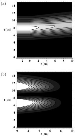
Figure 6: Contour plots of the intensities of the incoming (a) and the reflected (b) pulse. The medium stretches from $z=0$ to $z=10\,$cm, the frequency width of the incoming pulse is given by $\sigma_{\omega}=5\times 10^{5}\,\text{s}^{-1}$. We consider a gas of Rubidium atoms with a mean atomic density of $\bar{\rho}=2\times 10^{10}\,\text{cm}^{-3}$, a Rabi frequency of $\Omega_{p}=10^{7}\,s^{-1}$ and a zero detuning ($\omega_{p}=\omega_{0}$) for the pump lasers. The trajectory of the incoming pulse in (a) shows a bend at $z=0$. This is a consequence of the reduced group velocity inside the medium.

VI Quantization of the signal field

To see how a VSCPT gas influences the quantum state of the signal beams we consider the evolution of the field operator for the two signal modes interaction ,

$$\hat{\mbox{\boldmath$D$\unboldmath}}_{\text{s}}:=\varepsilon_{0}\,i\mathcal{E}_{\omega_{s}}\sum\limits_{i=1}^{2}a_{i}(t)\mbox{\boldmath$\epsilon$\unboldmath}_{i}e^{ik_{i}z}+\mbox{H.c.}\;,$$ (42)

where the modes are characterized by $k_{1}=k_{s}$, $k_{2}=-k_{s}$ and $\mbox{\boldmath$\epsilon$\unboldmath}_{1}=\mbox{\boldmath$\epsilon$\unboldmath}^{(+)}$ as well as $\mbox{\boldmath$\epsilon$\unboldmath}_{2}=\mbox{\boldmath$\epsilon$\unboldmath}^{(-)}$. We have set $\mathcal{E}_{\omega_{s}}:=\sqrt{\hbar\omega_{s}/(2\varepsilon_{0}V)}$ with $V$ being the quantization volume. We seek a solution to Heisenberg’s equation of motion for the (transverse) displacement $\hat{\mbox{\boldmath$D$\unboldmath}}_{\text{s}}$, which takes on the form

$$\left[\frac{1}{c^{2}}\partial_{t}^{2}-\Delta\right]\hat{\mbox{\boldmath$D$\unboldmath}}_{\text{s}}=\nabla\times\nabla\times\hat{\mbox{\boldmath$P$\unboldmath}}_{\text{s}}\;,$$ (43)

where $\hat{\mbox{\boldmath$P$\unboldmath}}_{\text{s}}:=\mbox{Tr}_{\text{R}}(\varrho_{\text{R}}\hat{\mbox{\boldmath$P$\unboldmath}})$ as well as $a_{i}(t)$ are reduced Heisenberg operators decoherence . The trace runs over all atomic and radiation degrees-of-freedom except for the two signal modes. It turns out that the operator $\hat{\mbox{\boldmath$P$\unboldmath}}_{\text{s}}$ has the same form as the classical polarization (III) if one replaces the Rabi frequencies $\Omega_{1,2}$ by $id\mathcal{E}_{\omega_{s}}a_{1,2}/\hbar$. Introducing the slowly varying operators $\tilde{a}_{i}(t):=a_{i}(t)\exp(i\omega_{s}t)$ one can derive the coupled set of first-order differential equations

$$\partial_{t}\left(\begin{array}[]{c}\tilde{a}_{1}\\ \tilde{a}_{2}\end{array}\right)=i\beta\left(\begin{array}[]{rr}-1&1\\ 1&-1\end{array}\right)\left(\begin{array}[]{c}\tilde{a}_{1}\\ \tilde{a}_{2}\end{array}\right)\;,$$ (44)

where second derivatives of the operators $\tilde{a}_{1,2}$ have been neglected against $\omega_{s}\dot{\tilde{a}}_{1,2}$. The coefficient $\beta$ is given by $\beta:=c\,n_{x}$, where $n_{x}$ can be either $n_{0}$ of Eq. (25) or $n_{p}$ of Eq. (35). We arrive at the following expression for the reduced annihilation operators

$$a_{1}(t) = e^{-i(\beta+\omega_{s})t}\,\left[\cos(\beta t)\,a_{1}+i\sin(\beta t)\,a_{2}\right]$$ (45)

$$a_{2}(t) = e^{-i(\beta+\omega_{s})t}\,\left[i\sin(\beta t)\,a_{1}+\cos(\beta t)\,a_{2}\right]\;,$$

where the operators $a_{i}$ on the right hand side are annihilation operators in the Schrödinger picture. The operators $a_{i}(t)$ do not obey the canonical commutation relations since $\beta$ is a complex parameter. This result is consistent, since canonical commutation relations are not required for reduced Heisenberg operators decoherence .

Solution (45) demonstrates that a single photon in the incoming signal beam $a_{1}$ will evolve into a superposition of the two signal modes. Such a state corresponds to single-particle entanglement, since the polarization and position degrees-of-freedom of the photon are then entangled. Hence, the one-particle entanglement which is present in the atomic VSCPT state can be transferred to a corresponding entanglement of a photon in a weak signal pulse. We remark that, apart from the possible appearance of EIT, the creation of single-particle entanglement could also be achieved by a beam splitter followed by a polarization rotator in one of the two output modes. The distinguishing feature of the VSCPT gas is that this effect is a direct signal of atomic entanglement.

In conclusion, we have shown that an atomic gas prepared in a VSCPT state exhibits unique optical features which include the phenomenon of EIT and a backscattered light pulse which is a signal for the entanglement associated with the VSCPT state. Detection of the backscattered light pulse should be possible for a gas of Rubidium atoms, while the large recoil velocity in Helium would make such an experiment unfeasible. On the few-photon level, the VSCPT gas would lead to single-particle entanglement for a signal photon.

Acknowledgments We would like to thank B. C. Sanders for fruitful discussions. This work was supported by the German Academic Exchange Service (DAAD) and Alberta’s informatics Circle of Research Excellence (iCORE).

References

• (1) A. Aspect, E. Arimondo, R. Kaiser, N. Vansteenkiste, and C. Cohen-Tannoudji, Phys. Rev. Lett. 61, 826 (1988).
• (2) T. Esslinger, F. Sander, M. Weidemüller, A. Hemmerich, T.W. Hänsch, Phys. Rev. Lett. 76, 2432 (1996).
• (3) J. Lawall, F. Bardou, B. Saubamea, K. Shimizu, M. Leduc, A. Aspect, and C. Cohen-Tannoudji, Phys. Rev. Lett. 73, 1915 (1994).
• (4) J. Lawall, S. Kulin, B. Saubamea, N. Bigelow, M. Leduc, and C. Cohen-Tannoudji, Phys. Rev. Lett. 75, 4194 (1995).
• (5) K. Bergmann, H. Theuer, and B. W. Shore, Rev. Mod. Phys. 70, 1003 (1998).
• (6) L. V. Hau, S. E. Harris, Z. Dutton, and C. H. Behroozi, Nature 397, 594 (1999).
• (7) D. F. Phillips, A. Fleischhauer, A. Mair, R. L. Walsworth, M. D. Lukin, Phys. Rev. Lett. 86, 783 (2001).
• (8) M. Fleischhauer and M. D. Lukin, Phys. Rev. Lett. 84, 5094 (2000).
• (9) C. Affolderbach, S. Knappe, R. Wynands, A. V. Taichenachev, and V. I. Yudin, Phys. Rev. A 65, 43810, (2002)
• (10) A. Aspect, E. Arimondo, R. Kaiser, N. Vansteenkiste, and C. Cohen-Tannoudji, Journ. Opt. Soc. Am. B 6, 2112 (1989).
• (11) C. Cohen-Tannoudji, Frontiers in Laser Spectroscopy, Editors: R. Balian, S. Haroche and S. Liberman (Amsterdam: North-Holland), 1977.
• (12) S. Stenholm, Appl. Phys. 15, 287 (1977).
• (13) To a first approximation the population of the excited and the bright state (the one that is orthogonal to $|\,D(p)\,\rangle$) can be neglected.
• (14) Since the equation for $\varrho_{1}$ is an inhomogeneous differential equation with an inhomogeneity linear in $E_{1}$ and $E_{2}$, one can simply treat the two cases separately and add the two inhomogeneous solutions afterwards.
• (15) The paraxial approximation for $\mbox{\boldmath$E$\unboldmath}_{2}$ takes on a different form than for $\mbox{\boldmath$E$\unboldmath}_{1}$ since $k_{2}^{2}c^{2}\not=\omega_{s}^{2}$. Terms of the order of magnitude $\Delta k^{2}/k_{s}$ have been neglected.
• (16) Maxwell’s equations impose boundary conditions on the electric and magnetic fields $E$ and $B$ at $z=0$ and $z=a$ which result in a reflection of the fields at these boundaries. In the paraxial approximation, this reflection is negligible and the boundary conditions for the electric field reduce to Eq. (26).
• (17) D. A. Steck, Rubidium 87 D Line Data,
http://steck.us/alkalidata/
• (18) M. Kasevich and S. Chu, Phys. Rev. Lett. 69, 1741 (1992).
• (19) The time dependence of the amplitudes $E_{1,2}$ has not been taken into account in the calculations for the denity operator. This amounts to ommit the changed group velocity of the pulse within the gas.
• (20) M. O. Scully, M. S. Zubairy, Quantum Optics, Cambridge University Press (1995).
• (21) C. Liou, Z. Dutton, C. H. Behroozi, and L. V. Hau, Nature 409, 490 (2001).
• (22) M. D. Lukin, S. F. Yelin, and M. Fleischhauer, Phys. Rev. Lett. 84, 4232 (2000).
• (23) Since we describe the atom-field interaction in multipolar coupling, it is advantageous to deal with the transverse displacement $\hat{\mbox{\boldmath$D$\unboldmath}}_{\text{s}}$ instead of the electric field itself; see, for example, J.R. Ackerhalt and P.W. Milonni, J. Opt. Soc. Am. B 1, 116 (1984).
• (24) K.-P. Marzlin, Phys. Rev. A 64, 011405(R) (2001).