The most robust entangled state of light

Abstract

We study how photon absorption losses degrade the bipartite entanglement of entangled states of light. We consider two questions: (i) what state contains the smallest average number of photons given a fixed amount of entanglement? and (ii) what state is the most robust against photon absorption? We explain why the two-mode squeezed state is the answer to the first question but not quite to the second question.

I Introduction

For long-distance quantum communication the most important decoherence mechanism is due to photon absorption. It would be nice to know what type of entangled states of light is most robust, i.e. preserves its entanglement best, against photon absorption losses. Intuitively one might think that states containing fewer photons will be more robust. After all, both loss rates and decoherence rates tend to increase with the number of photons. For instance, a cavity filled with exactly $N$ photons loses photons at a rate proportional to $N$. Similarly, it is well known that, in general, the more macroscopic a state is the more sensitive it is to noise. For example, the decoherence rate of Schrödinger cat states of the (unnormalized) form

$$|\alpha\rangle\pm|-\alpha\rangle,$$ (1)

with $|\alpha\rangle$ a coherent state, increases with the amplitude $|\alpha|$. This phenomenon was demonstrated experimentally in the context of microwave cavity-QED haroche and for motional states of ions in an ion trap myatt . Also entangled coherent states of the (unnormalized) form

$$|\alpha\rangle|\alpha\rangle-|-\alpha\rangle|-\alpha\rangle,$$ (2)

decohere faster with increasing $|\alpha|$. This fact was discussed in several theoretical papers: Ref. hirota uses an operational measure and shows that the teleportation fidelity decreases monotonically with $|\alpha|$, and another paper lixu demonstrates that the entanglement of formation decreases monotomically with $|\alpha|$ as well.

If the intuition that a smaller number of photons makes a state more robust were true, then the most robust entangled state of light would be the two-mode squeezed state. That state contains the smallest average number of photons given a fixed amount of entanglement, as we will show in Section II. We will see, however, that the intuitive answer is not quite correct and we will explain why this is so in Section III. The calculations in Section III proceed as follows: we consider large classes of pure states (both Gaussian and non-Gaussian states) with a fixed amount of entanglement. Then we calculate the entanglement that remains after those states have decohered by being subjected to photon absorption. That remaining entanglement is considered to be a measure of the robustness of the entangled state against photon absorption. The robustness is investigated as a function of the average number of photons in the initial pure state. We use two definitions of entanglement, the entanglement of formation and the negativity. In the former case we restrict our attention to states for which the entanglement of formation can be calculated analytically, in the latter case there is no restriction on the types of states considered.

We end this Introduction by noting that the entanglement of a state of the electromagnetic field is completely determined by its expansion in Fock (photon number) states pz . Consequently, the effects of photon absorption losses on the entanglement of a state are likewise completely determined by the form of the state in the Fock basis. On the other hand, the effects of other decoherence mechanisms arising from, say, polarization diffusion or phase diffusion, depend on the physical implementation of the state. For example, if one uses two modes that are different only in their polarization degree of freedom, then polarization diffusion mixes the two modes. But if the two modes are spatially separated then no such mixing occurs. The type of decoherence discussed in the present paper is thus the most universal type of decoherence of entangled states of light, in the sense that it is independent of the precise physical implementation of the state.

II Photons and entanglement

Let us consider a bipartite system consisting of two spatially separated electromagnetic field modes $A$ and $B$. The entanglement in a pure state on $A$ and $B$ is given by the von Neumann entropy of the partial density matrix of either system $A$ or $B$, where the pure state can be written in the photon-number basis as

$$|\Psi\rangle_{A,B}=\sum_{n,m=0}^{\infty}\alpha_{nm}|n\rangle_{A}|m\rangle_{B}.$$ (3)

The problem of finding the state with the smallest average number of photons for a fixed amount of entanglement is mathematically equivalent to a well-known problem from thermodynamics: finding the state with the largest entropy given a fixed energy, which is, almost obviously, the same as finding the state with the smallest energy given a fixed entropy. Indeed, energy is proportional to the average number of photons, and the entropy is just the entanglement. The answer to the thermodynamics question is of course the thermal state. That is, the state

$$\rho=(1-\lambda)\sum_{n}\lambda^{n}|n\rangle\langle n|$$ (4)

maximizes the entropy for fixed average energy, where $\lambda=\exp(-\hbar\omega/kT)$ if $n\hbar\omega$ is the energy of the state $|n\rangle$ and $T$ the temperature. But that mixed state arises indeed from a two-mode squeezed state of the form

$$\sqrt{1-|\gamma|^{2}}\sum_{n}\gamma^{n}|n\rangle|n\rangle,$$ (5)

for any $\gamma$ for which $|\gamma|^{2}=\lambda$. In particular, the entanglement in this state is

$$E=(\frac{\bar{n}}{2}+1)\log_{2}(\bar{n}+2)-\bar{n}\log_{2}\bar{n}-1,$$ (6)

in terms of the average number of photons

$$\bar{n}=\frac{2\lambda}{1-\lambda}=\frac{2|\gamma|^{2}}{1-|\gamma|^{2}}.$$ (7)

For instance, for $\bar{n}=1$ one has more than one unit of entanglement, as $E=3\log_{2}(3)/2-1\approx 1.3774$. Conversely, it takes less than one photon ($0.5876$ of a photon to be more precise) to have one ebit of entanglement between two modes. That might seem surprising as one might have expected the state $|0\rangle|1\rangle+|1\rangle|0\rangle$, a state with one photon and one ebit of entanglement, to maximize the entanglement of one photon in two modes.

If one allows an arbitrarily large number of modes for both parties, it is straightforward to get an arbitrarily large amount of bipartite entanglement. For example, consider states with two photons: with $M$ modes for each party, the bipartite state $|1000\ldots 1000\ldots\rangle+|0100\ldots 0100\ldots\rangle+|0010\ldots 0010\ldots\rangle+\ldots$ has exactly $\log_{2}(M)$ ebits of entanglement. But the state that maximizes the amount of entanglement in the case of $M$ modes for both parties for two photons contains more than twice as much entanglement and is simply a tensor product of $M$ two-mode squeezed states each with average photon number $2/M$, with a total entanglement of $2\log_{2}(M)+1+{\cal O}(1/M)$ for large $M$.

III Entanglement of decohered states

In this Section we will consider the most robust bipartite state of just two modes. This should reveal most properties of multi-mode entangled states under the assumption that all modes decohere independently and identically. In particular, we assume the following model for photon absorption losses: For any coherent state $|\alpha\rangle_{A}$ of a mode $A$, photon absorption is governed by the process

$$|\alpha\rangle_{A}|0\rangle_{E}\mapsto|\sqrt{\eta}\alpha\rangle_{A}|\sqrt{1-\eta}\alpha\rangle_{E},$$ (8)

where $E$ denotes the environment, which is assumed to be unobservable and hence must be traced out. The parameter $\eta$ gives the fraction of photons in mode $A$ that survives the photon absorption process, with $\eta=1$ thus corresponding to a noiseless channel. Since coherent states form an overcomplete set of states, the model (8) fully specifies decoherence due to photon absorption. We assume that all modes decohere in the same way, according to (8), with the same parameter $\eta$ for each mode and a different environment for each mode.

A pure state of the form (3) is turned into a mixture by the photon absorption process (8). Calculating the entanglement of a general mixed state is no trivial problem, as is well known. We follow two paths here in order to find the entanglement that remains after photon absorption.

In the first subsection we consider states for which we can analytically calculate the entanglement of formation for the mixed state that arises from photon absorption. This first of all includes all states in which each of the two modes $A$ and $B$ contain at most one photon. In that case the Hilbert space of each mode is two-dimensional, also after photon absorption, and we can apply the Wootters formula wootters . Secondly, we can consider the two-mode squeezed state, as it is a Gaussian state and remains Gaussian after photon absorption, so that we can apply the results of giedke . In the second subsection we consider arbitrary states and calculate (numerically) the negativity vidal1 ; vidal2 . Here too, analytical calculations become tedious or impossible depending on the dimension of the matrix whose eigenvalues have to be calculated.

In both subsections we consider states with a fixed amount of entanglement and wish to find the states that preserve their entanglement best under photon absorption.

III.1 Entanglement of formation

We first consider states of the general form

$$\sqrt{p}|\phi\rangle_{A}|\varphi\rangle_{B}+\sqrt{1-p}|\phi^{\perp}\rangle_{A}|\varphi^{\perp}\rangle_{B},$$ (9)

where the parameter $0\leq p\leq 1/2$ fully determines the entanglement of formation of the state

$$E=-p\log_{2}(p)-(1-p)\log_{2}(1-p),$$ (10)

and where

$$|\phi\rangle_{A} = \cos\alpha|0\rangle+\sin\alpha|1\rangle$$

$$|\varphi\rangle_{B} = \cos\beta|0\rangle+\sin\beta|1\rangle$$

$$|\phi^{\perp}\rangle_{A} = -\sin\alpha|0\rangle+\cos\alpha|1\rangle$$

$$|\varphi^{\perp}\rangle_{B} = -\sin\beta|0\rangle+\cos\beta|1\rangle$$ (11)

form arbitrary orthonormal bases in the subspaces spanned by the zero- and one-photon states in modes $A$ and $B$. We then fix $p$ and $\eta$ and plot the entanglement of all states of the form (9) after they have lost a fraction $1-\eta$ of their photons by varying the angles $\alpha$ and $\beta$ independently. We plot the result as a function of the average number of photons $\bar{n}$ in the original undecohered pure state (9),

$$\bar{n}=p(\cos^{2}\alpha+\cos^{2}\beta)+(1-p)(\sin^{2}\alpha+\sin^{2}\beta).$$ (12)

Results for specific parameters are plotted in Fig. 1.

Figure 1: Entanglement of formation as a function of the average number of photons (in both modes combined) for all bipartite states with at most one photon in each mode.

In particular, we choose $\eta=0.5$ and fix $p=1/3$, so that the entanglement of formation of the pure state is $E\approx 0.9183$. The optimum state is found to be

$$\sqrt{p}|01\rangle-\sqrt{1-p}|10\rangle,$$ (13)

which contains one photon and for which the entanglement left after decoherence is $E\approx 0.3236$. Now clearly, this optimum is not obtained for the smallest average number of photons, which is 2/3 for the states (9) considered. That minimum average number of photons is attained for the state

$$\sqrt{p}|11\rangle-\sqrt{1-p}|00\rangle,$$ (14)

but its entanglement after decoherence is only $E\approx 0.1622$. (One notices the similarity of the state (14) and the two-mode squeezed state.) These two facts clearly refute the intuition that a lower number of photons should lead to less decoherence. On the other hand, it is true that the state with the largest amount of photons, 4/3, decoheres the most. That is, in the state

$$\sqrt{1-p}|11\rangle+\sqrt{p}|00\rangle$$ (15)

the amount of entanglement surviving the 50% photon absorption is $E\approx 0.0438$. The minimum entanglement after decoherence for a fixed average number of photons is in fact obtained for the family of states for which $\alpha=\beta$.

In order to explain the preceding results, let us give an intuitive idea for why the state

$$\sqrt{1/2}|11\rangle+\sqrt{1/2}|00\rangle$$ (16)

is less robust (when using the entanglement of formation as entanglement measure) than the state

$$\sqrt{1/2}|10\rangle+\sqrt{1/2}|01\rangle,$$ (17)

although both states contain 1 photon on average. For concreteness, again assume we lose 50% of the photons. Suppose we would be able to measure the number of photons in the two environments into which the two modes decohere (with a perfect photon detector). In that case, if we don’t find any photons we know we have an entangled state of the two modes, whereas if we do find a photon in the environment, we have no entanglement left between the two modes. In the case of the state (16) we have a probability of $(1+\eta^{2})/2=5/8$ to find no photons in the environment, but the state of the two modes is collapsed onto the (unnormalized) state

$$\sqrt{1/2}|11\rangle+\sqrt{1/2}\eta|00\rangle$$ (18)

with an entanglement of $E\approx 0.72$ for $\eta=1/2$. On the other hand, for the state (17) we have a slightly smaller chance of $\eta=1/2$ to find no photons in the environment, but the state of the two modes then collapses back onto (17), with its full entanglement of 1 ebit. Thus on average we indeed retain more entanglement from state (17) (namely 0.5 ebits) than from (16) (namely, 0.45 ebits) after decoherence, making (17) the more robust state. This then also indicates why the family of states (13) are more robust than either of the families of states (14) and (15).

A second type of states for which the entanglement of formation after decoherence can be calculated is the set of entangled coherent states. The reduced density matrix of those states has rank two, the support given by the two-dimensional Hilbert space spanned by two different coherent states, which we choose here as $|\alpha\rangle$ and $|-\alpha\rangle$. After decoherence the relevant Hilbert space remains two-dimensional, spanned by coherent states $|\pm\sqrt{\eta}\alpha\rangle$. We can distinguish three types of states. The first two are both symmetric under the interchange of the two modes $A$ and $B$,

$$\sqrt{p}|+\rangle_{A}|+\rangle_{B}+\sqrt{1-p}\exp(i\phi)|-\rangle_{A}|-\rangle_{B},$$ (19)

with $0\leq p\leq 1/2$, and

$$\sqrt{1-p}|+\rangle_{A}|+\rangle_{B}+\sqrt{p}\exp(i\phi)|-\rangle_{A}|-\rangle_{B}.$$ (20)

The third type is of the general form

$$\sqrt{p}|+\rangle_{A}|-\rangle_{B}+\sqrt{1-p}\exp(i\phi)|-\rangle_{A}|+\rangle_{B}.$$ (21)

Here the $|\pm\rangle$ states are defined by

$$|\pm\rangle = (|\alpha\rangle\pm|-\alpha\rangle)/\sqrt{N_{\pm}}$$

$$N_{\pm} = 2\pm 2\exp(-2|\alpha|^{2}),$$ (22)

which form an orthonormal basis for the relevant Hilbert space. Just as before we choose $p=1/3$ and $\eta=1/2$. The entanglement left after decoherence is plotted in Fig. 2 for various values of the phase $\phi$. One clearly identifies three groups of curves. They correspond to the states (19), (20), and (21). In particular, the states with the largest amount of entanglement correspond to (21), and the states with the smallest and largest numbers of photons, respectively, to (19) and (20). Within each group the states have the property that fewer photons lead to less decoherence. On the other hand, the state with the largest amount of entanglement is not the state with the smallest number of photons. The three optimal states within the three groups are the same three states singled out above, (13), (14), and (15), and correpond to the limit $\alpha\rightarrow 0$.

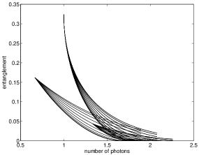
Figure 2: Entanglement of formation as a function of the average number of photons for three types of entangled coherent states (19), (20) and (21).

We can infer two conclusions from the results plotted in Figs. 1 and 2 that make it seem unlikely the two-mode squeezed state would be the most robust. First, states with fewer photons are not more robust, and second, the symmetric states of the two modes are not the most robust either.

Nevertheless, if we consider the two-mode squeezed state with the same amount of entanglement as the other states discussed in this subsection, then we find, using the formula for the entanglement of symmetric Gaussian states from giedke , the average number of photons in the state and the entanglement left after decoherence are, respectively, $\bar{n}\approx 0.5138$ and $E\approx 0.3979$, thus clearly improving on the most robust states considered above. Unfortunately, without being able to calculate the entanglement of formation for more complicated states or states with fewer symmetry properties or living in larger Hilbert spaces, it is not possible to conclude anything yet about the two-mode squeezed state being the most robust entangled state of light in this context. That is the main reason to consider a measure of entanglement that can be calculated easily for any type of entangled state, the negativity vidal1 ; vidal2 .

III.2 Negativity

Suppose we have an arbitrary pure state of two modes $A$ and $B$. We can always write this state in its Schmidt decomposition,

$$|\Psi\rangle_{AB}=\sum_{k}c_{k}|\phi_{k}\rangle_{A}|\varphi_{k}\rangle_{B},$$ (23)

with the $c_{k}$ real positive coefficients with $\sum c_{k}^{2}=1$, and $|\phi_{k}\rangle_{A}$ and $|\varphi_{k}\rangle_{B}$ orthonormal states on systems $A$ and $B$. The negativity of a pure state can be defined in terms of the Schmidt coefficients as

$$N=\frac{1}{2}\big{(}[\sum_{k}c_{k}]^{2}-1\big{)}.$$ (24)

For a mixed state the negativity is determined by the sum of the absolute values of the negative eigenvalues of the partial transpose of the density matrix vidal2 . Numerically, we expand each density matrix in number states and then the partial transpose (with respect to system $A$) is defined as

$$\langle n_{A},n_{B}|\rho^{T_{A}}|m_{A},m_{B}\rangle=\langle m_{A},n_{B}|\rho|n_{A},m_{B}\rangle,$$ (25)

and the negativity is then

$$N(\rho)=\frac{||\rho^{T_{A}}||-1}{2},$$ (26)

with $||.||$ denoting the trace norm. We are interested in fixing the entanglement of a pure state and then calculating the negativity of the decohered state. Since we have now considered two different measures of entanglement, we will in fact always fix both the entanglement of formation and the negativity of the pure states. This is done as follows: suppose we are looking for a state with $M$ Schmidt coefficients $c_{1}\ldots c_{M}$ with $M\geq 4$ and a fixed value $E$ for the entanglement of formation and a fixed value $N$ for the negativity. If we treat $c_{3}\ldots c_{M}$ as fixed, then $c_{1}$ and $c_{2}$ are determined by the normalization and $N$. Since both the negativity and the norm are simple functions of the Schmidt coefficients we can in fact determine $c_{1}$ and $c_{2}$ analytically. The entanglement of formation is not a simple function, and so we use a numerical method to determine coefficients $c_{1}\ldots c_{3}$ given coefficients $c_{4}\ldots c_{M}$. Namely, we use Newton’s method to obtain better and better estimates of $c_{3}$, such that the entanglement of formation approaches $E$, where for each $c_{3}$ the coefficients $c_{1}$ and $c_{2}$ are fixed analytically.

We first consider the most straightforward case, where we in fact keep all Schmidt coefficients the same as for a two-mode squeezed state, but vary the basis vectors $|\phi_{k}\rangle_{A}$ and $|\varphi_{k}\rangle_{B}$ in the Schmidt decomposition (24). An arbitrary $M$-dimensional basis can be fully be specified by $M-1$ angles, in analogy to the 2 Euler angles in 3-D space. We choose the definitions of the angles such that the number state basis $|0\rangle,|1\rangle,\ldots|M-1\rangle$ corresponds to setting all angles equal to zero. Instead of varying those basis vectors over all possible choices by varying all angles over $2\pi$ independently, we instead choose, for computational efficiency reasons, a large number of randomly chosen basis vectors by choosing randomly $M-1$ angles. In order to choose random states that are within a certain “distance” from the standard Fock basis we simply restrict the maximum values of the $M-1$ angles. By increasing the distance one can get further and further away from the two-mode squeezed state. In Figs 3 and 4 we plot the results. We plot the negativity of the decohered state as a function of the average photon number in the pure state for two different distances. The first restricts the angles to be less than 1/10, in Fig. 4 the distance is unrestricted. The two-mode squeezed state we take has the same entanglement of formation as before, and $\eta=0.5$, also as before. The Schmidt coefficients of the two-mode squeezed state become exponentially smaller with the number of photons $n$ (see (5). Hence, if we truncate the Hilbert space at a certain maximum photon number $N_{m}$, the state thus obtained is a good approximation to a two-mode squeezed state provided $N_{m}$ is sufficiently large. Here we chose $N_{m}=6$. This means that by varying the basis states, the maximum possible number of photons is, of course, at most 6, as indeed is clear in Fig. 4.

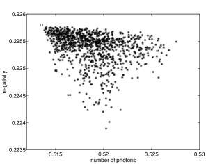
Figure 3: Negativity as a function of average number of photons for 1000 randomly generated states whose Schmidt coefficients are equal to that of a two-mode squeezed state, with a restriction on the distance from a two-mode squeezed state, as explained in the text. The circle indicates the two-mode squeezed state.

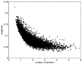
Figure 4: Same as previous Figure, except there is no restriction on the distance to the two-mode squeezed state.

What we see from the two figures is that indeed the two-mode squeezed state itself is the most robust among the set of states considered here, which can be confirmed numerically by decreasing the distance even more than in Fig. 3.

It is probably worthwhile noting that all entanglement properties of a given state are determined by the Schmidt coeffcients. And so the conclusion is that, with all entanglement properties being equal, the state with the smallest number of photons is the most robust, provided we use the negativity of the decohered state to measure robustness.

As an aside we note it might be slightly confusing to read in Ref. vidal1 that the negativity of any state, mixed or pure, is proportional to the “robustness” of entanglement. However, the two definitions of the word “robustness” are quite different. In vidal1 the robustness of the entanglement of a state refers to how much of unentangled states on the $M$-dimensional Hlbert space has to be mixed with the original state in order to remove all entanglement from the state.

We can try to confirm the behavior of the negativity for the same set of states that featured in Fig. 1, i.e., the states with at most one photon in each mode $A$ and $B$.

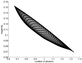
Figure 5: Negativity as a function of the average number of photons for states of the form (9).

One sees that the negativity, in contrast to the entanglement of formation (See Fig. 1), does seem to favor states with fewer photons as far as robustness is concerned.

On the other hand, there are states that do have the same amount of entanglement of formation and the same negativity as the two-mode squeeze state, but do not have the same Schmidt coefficients. For those states there necessarily exist at least one measure of entanglement that is different than that for the two-mode sqeezed state. Let us investigate this a little further. If we restrict the Hilbert space of both modes $A$ and $B$ to contain at most three photons, then there are at most four Schmidt coefficients. The coefficients are then fixed by the normalization, by the negativity, by the entanglement of formation, and by some third measure of entanglement, i.e. some other independent function of the Schmidt coefficients $c_{k}$. For instance, let us, quite arbitrarily, choose the purity of the reduced density matrix as the third entanglement measure,

$$P=1-\sum(c_{k}^{4}).$$ (27)

We then take a two-mode squeezed state but truncate its Fock-state expansion after four terms. In order for it to be a good approximation to an actual two-mode squeezed state we choose the average number of photons and the entanglement smaller than we did in previous examples.

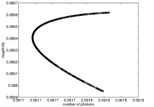
Figure 6: Negativity as a function of the average number of photons for states with fixed pure-state negativity and entanglement of formation and at most containing three photons per mode.

In Fig. 6 we plot the negativity of the decohered states (again using $\eta=0.5$) as a function of the average number of photons for 1000 randomly generated states that all have the same pure-state entanglement $E=0.2$ and negativity $N=0.2079$. The plot then shows that there is indeed a line of points, indicating there is exactly one more function characterizing the initial pure state.

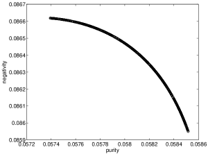
Figure 7: Negativity as a function of the purity for states with fixed pure-state negativity and entanglement of formation and at most containing three photons per mode.

In Fig. 7, then, we plot the same data but as a function of the purity $P$, which then indeed shows a monotonic behavior, rather than the bistable behavior of Fig. 7. In fact, it shows, perhaps surprisingly, that the smaller the purity, the more robust the state. From Figs  6 and 7 it follows already that the two-mode squeezed state is not the most robust entangled state of light, although it is close in the sense that the entanglement of the most robust state is only a trifle larger than that of the two-mode squeezed state.

We extend this discussion to states confined to rank five, containing at most four photons. The corresponding plots are in Figs. 8 and 9.

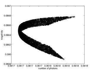
Figure 8: Same as Fig. 6 except for states with at most four photons.

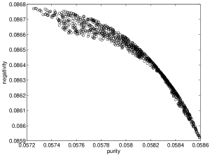
Figure 9: Same as Fig. 7 except for states with at most four photons.

Those plots show that, as expected, there is now more than one extra degree of freedom (in this case exactly two degrees of freedom, of course) that determines how robust a given entangled state is. But the extra degrees of freedom, in this example, hardly increase (less than 0.1%) the negativity of the decohered state relative to that of the two-mode squeezed state. This is because the states we considered have only a small projection onto the extra dimensions (i.e., the Fock states with 3 and 4 photons). If we increase the amount of entanglement and, concomittantly, the allowed average number of photons in the initial state, the extra degrees of freedom should become more important. For example, taking states with an entanglement of $E\approx 0.82$ leads to an average number of photons of $\bar{n}\approx 0.5137$ for the two-mode squeezed state, and the most robust state then turns out to be 2% more robust than the two-mode squeezed state. The optimum state has in that case an average photon number of $\bar{n}\approx 0.5797$, as was found numerically. Thus, we expect the two-mode squeezed state (5) to be close to the most robust entangled state of light if its entanglement and average number of photons are small. For reasonable (i.e., experimentally achievable) values the robustness is always clearly within 1% of the optimum.

IV Discussion

In this paper we considered the degradation of entanglement of entangled states of light suffering from photon absorption losses. The aim was to find the most robust entangled state, i.e., the state that preserves its entanglement best under a given amount of noise. We found that the answer depends on how one formulates the problem. In particular, it depends on what measure(s) of entanglement one uses. That is, we may fix any number $n$ of entanglement measures $M_{1}\ldots M_{n}$ of the initial pure state and use one particular entanglement measure $M_{0}$ of the decohered state (after photon absorption) to define the robustness of the state. The answer which state is the most robust then depends on the measures $M_{0}$ and $M_{1}\ldots M_{n}$ one uses.

If one fixes two measures of entanglement and takes $M_{1}$ to be the entanglement of formation and $M_{2}$ the negativity, and one uses the negativity for $M_{0}$, we found that states with smaller number of photons tend to be more robust. Nevertheless, the most robust state is not the state with the smallest possible number of photons, the two-mode squeezed state. The reason is that even when one fixes both the entanglement of formation and the negativity there are still other degrees of freedom left that determine the entanglement properties of the pure state, including its robustness against photon absorption losses. The two-mode squeezed state is close to the most robust state, though, and is very close for experimentally achievable parameters. That is, the value of $M_{0}$ for the most robust state differs less than 1% from that of the two-mode squeezed state for realistic parameters.

On the other hand, if one fixes all entanglement degrees of freedom of a pure state (i.e. all Schmidt coefficients) and uses the negativity of the decohered state to quantify robustness, then the most robust state is the one with the smallest (given all constraints) number of photons.

References

- (1) J.M. Raimond, M. Brune, and S. Haroche, Phys. Rev. Lett. 79, 1964 (1997).
- (2) C.J. Myatt et al., Nature 403, 269 (2000).
- (3) S.J. van Enk and O. Hirota, Phys. Rev. A 64, 022313 (2001).
- (4) S-B Li and J-B Xu, Phys. Lett. A 309, 321 (2003).
- (5) P. Zanardi, Phys. Rev. A 65, 042101 (2002); S.J. van Enk, Phys. Rev. A 67, 022303 (2003); Y. Shi, Phys. Rev. A 67, 024301 (2003).
- (6) W.K. Wootters, Phys. Rev. Lett. 80, 2245 (1998).
- (7) G. Giedke et al., Phys. Rev. Lett. 91, 107901 (2003).
- (8) G. Vidal and R. Tarrach, Phys. Rev. A 59, 141 (1999).
- (9) G. Vidal and R.F. Werner, Phys. Rev. A 65, 032314 (2002).