The Cosmic Microwave Background Bipolar Power Spectrum:
Basic Formalism and Applications

Abstract

We study the statistical isotropy (SI) of temperature fluctuations of the CMB as distinct from Gaussianity. We present a detailed formalism of the bipolar power spectrum (BiPS) which was introduced as a fast method of measuring the statistical isotropy by Hajian & Souradeep 2003. The method exploits the existence of patterns in the real space correlations of the CMB temperature field. We discuss the applications of BiPS in constraining the topology of the universe and other theoretical scenarios of SI violation. Unlike the traditional methods of search for cosmic topology, this method is computationally fast. We also show that BiPS is potentially a good tool to detect the effect of observational artifacts in a CMB map such as non-circular beam, anisotropic noise , etc. Our method has been successfully applied to the Wilkinson Microwave Anisotropy Probe sky maps by Hajian et al. 2004, but no strong evidence of SI violation was found.

1 Introduction

The first-year Wilkinson Microwave Anisotropy Probe (WMAP) observations are consistent with predictions of the concordance $\Lambda$CDM model with scale-invariant and adiabatic fluctuations which have been generated during the inflationary epoch Hinshaw et al. (2003); Kogut et al. (2003); Spergel et al. (2003); Page et al. (2003); Peiris et al., (2003). After the first year of WMAP data, the SI of the CMB anisotropy (i.e. rotational invariance of n-point correlations) has attracted considerable attention. Tantalizing evidence of SI breakdown (albeit, in very different guises) has mounted in the WMAP first year sky maps, using a variety of different statistics. It was pointed out that the suppression of power in the quadrupole and octopole are aligned Tegmark et al. (2004). Further “multipole-vector” directions associated with these multipoles (and some other low multipoles as well) appear to be anomalously correlated Copi et al. (2004); Schwarz et al. (2004). There are indications of asymmetry in the power spectrum at low multipoles in opposite hemispheres Eriksen et al. 2004a ; Hansen et al. (2004); Naselsky et al. (2004). Possibly related, are the results of tests of Gaussianity that show asymmetry in the amplitude of the measured genus amplitude (at about $2$ to $3\sigma$ significance) between the north and south galactic hemispheres Park (2004); Eriksen et al. 2004b ; Eriksen et al. 2004c . Analysis of the distribution of extrema in WMAP sky maps has indicated non-gaussianity, and to some extent, violation of SI Larson & Wandelt (2004). However, what is missing is a common, well defined, mathematical language to quantify SI (as distinct from non Gaussianity) and the ability to ascribe statistical significance to the anomalies unambiguously.

In order to extract more information from the rich source of information provided by present (and future) CMB maps, it is important to design as many independent statistical methods as possible to study deviations from standard statistics, such as statistical isotropy (SI). Since SI can be violated in many different ways, various statistical methods can come to different conclusions. Because each method by design is more sensitive to a special kind of SI violation.

As a statistical tool of searching for departures from SI, we use the bipolar power spectrum (BiPS) which is sensitive to structures and patterns in the underlying total two-point correlation function Hajian & Souradeep 2003b ; Souradeep & Hajian (2003). The BiPS is particularly sensitive to real space correlation patterns (preferred directions, etc.) on characteristic angular scales. In harmonic space, the BiPS at multipole $\ell$ sums power in off-diagonal elements of the covariance matrix, $\langle a_{lm}a_{l^{\prime}m^{\prime}}\rangle$, in the same way that the ‘angular momentum’ addition of states $lm$, $l^{\prime}m^{\prime}$ have non-zero overlap with a state with angular momentum $|l-l^{\prime}|<\ell<l+l^{\prime}$. Signatures, like $a_{lm}$ and $a_{l+nm}$ being correlated over a significant range $l$ are ideal targets for BiPS. These are typical of SI violation due to cosmic topology and the predicted BiPS in these models have a strong spectral signature in the bipolar multipole $\ell$ space Hajian & Souradeep 2003a . The orientation independence of BiPS is an advantage since one can obtain constraints on cosmic topology that do not depend on the unknown specific orientation of the pattern (e.g., preferred directions).

In the rest of this section we briefly introduce some basic statistical properties of CMB and discuss the statistical isotropy as distinct from Gaussianity. In sections 2 and 3 we introduce BiPS in real as well as harmonic space. In section 4 and 5 we define an unbiased estimator for BiPS and compute its cosmic variance in details. In section 6 we briefly introduce some possible sources of breakdown of SI. In section 7 we discuss the results of applying the method to the simulations and WMAP data. We draw our conclusions in section 8. For completeness we have also included details of calculations in 6 appendices to keep the paper easily readable.

1.1 Statistical Properties of the CMB Anisotropy

The temperature anisotropies of the CMB are described by a random field, $\Delta T(\hat{n})=T(\hat{n})-T_{0}$, on a 2-dimensional surface of a sphere (the so called surface of last scattering), where $\hat{n}=(\theta,\phi)$ is a unit vector on the sphere and $T_{0}=\int{\frac{d\Omega_{\hat{n}}}{4\pi}T(\hat{n})}$ represents the mean temperature of the CMB. The statistical properties of this field can be characterized by the $n$-point correlation functions

$$\langle\Delta T(\hat{n}_{1})\Delta T(\hat{n}_{2})\cdots\Delta T(\hat{n}_{n})\rangle.$$ (1)

Here the bracket denotes the ensemble average, i.e. an average over all possible configurations of the field. If the field is Gaussian in nature, the connected part of the $n$-point functions disappears for $n>2$. The non-zero (even-$n$)-point correlation functions can be expressed in terms of the $2$-point correlation function. As a result, a Gaussian distribution is completely described by the two-point correlation function.

The statistics of the temperature fluctuations is Gaussian because they are linearly connected to quantum vacuum fluctuations of a very weakly interacting scalar field (the inflaton). Perturbations in primordial gravitational potential, $\Phi_{0}$, generate the CMB anisotropy, $\Delta T$. The linear perturbation theory gives a linear relation between $\Phi_{0}$ and $\Delta T$. $\Phi_{0}({\mathbf{x}})$ is assumed to be Gaussian, because in inflation, quantum fluctuations produce Gaussian random phase variations in the gravitational potential

$$\Phi_{0}({\mathbf{x}})=\int{\frac{{\mathrm{d}}^{3}{\mathbf{k}}}{(2\pi)^{3}}\Phi_{0}(\mathbf{k})\exp{i\mathbf{k}\cdot\mathbf{x}}}$$ (2)

with $\langle\Phi_{0}({\mathbf{k}})\Phi_{0}^{*}({\mathbf{k^{\prime}}})\rangle=P(k)\delta({\mathbf{k}}-{\mathbf{k^{\prime}}})$, the power spectrum of potential fluctuations at that epoch. In the linear temperature approximation, in a spatially flat universe, the temperature anisotropies at the surface of last scattering can be linearly related to the potential fluctuations at that epoch

$$\Delta T(\hat{n})=\int{\frac{{\mathrm{d}}^{3}{\mathbf{k}}}{(2\pi)^{3}}e^{i{\mathbf{k}}\cdot\hat{n}\tau_{rec}}\Phi_{0}({\mathbf{k}})g_{T}(k)},$$ (3)

where $\tau_{rec}$ is the comoving conformal lookback time of the recombination epoch ($\tau$ is the conformal time $\tau=\int{\mathrm{d}t/a}$), $\phi(\tau)$ is a normalization constant for potential perturbations which is equal to unity today, and $g_{T}(k)$ is the linear radiation transfer function which describes the relationship between potential fluctuations and temperature fluctuations at recombination. For small $k$, $g_{T}(k)=1/3$, which is known as the fact that for temperature fluctuations on super-horizon scales at the decoupling epoch, the Sachs-Wolfe effect Sachs and Wolfe, (1967) dominates and hence on large angular scales

$$\frac{\Delta T}{T}(\hat{n})\,=\,\frac{1}{3}\Phi_{LS}(\hat{n}\tau_{rec},\tau_{0})$$ (4)

On sub-horizon scales, $g_{T}$ oscillates (acoustic oscillation), and we need to evolve the coupled matter-radiation fluid, i.e. solve the Boltzmann photon transport equations coupled with the Einstein equations for $g_{T}$. Codes like CMBFAST compute $g_{T}(k)$ for different cosmological models.

If we expand the gravitational potential into a series in powers of a density enhancement

$$\Phi({\mathbf{x}},t)=\Phi^{(1)}+\Phi^{(2)}+\cdots$$ (5)

The linear term $\Phi^{1}=\Phi_{0}({\mathbf{x}})$ and is assumed to be Gaussian .Non-linearity in inflation makes $\Phi$ weakly non-Gaussian and will lead to non-linear terms, such as $\Phi^{(2)}$, in eqn. (5). However, since potential fluctuations in the early universe are small, $\langle\Phi^{2}\rangle\sim 10^{-9}$, these non-linear effects are usually viewed as undetectable Munshi et al. (1995); Spergel et al. (1999) (for a nice review on non-Gaussianity see Bartolo et al. (2004)). Hence, here we limit our study to Gaussian CMB anisotropy field, where the two-point correlation function

$$C(\hat{n},\,\hat{n}^{\prime})\equiv\langle\Delta T(\hat{n})\Delta T(\hat{n}^{\prime})\rangle$$ (6)

contains all the statistical information encoded in the field.

It is convenient to expand the temperature anisotropy field into spherical harmonics, the orthonormal basis on the sphere, as

$$\Delta T(\hat{n})\,=\,\sum_{l,m}a_{lm}Y_{lm}(\hat{n})\,\,,$$ (7)

where the complex quantities, $a_{lm}$ are given by

$$a_{lm}=\int{\mathrm{d}\Omega_{\hat{n}}Y_{lm}^{*}(\hat{n})\Delta T(\hat{n})}.$$ (8)

For a Gaussian CMB anisotropy, $a_{lm}$ are Gaussian random variables and hence, the covariance matrix, $\langle a_{lm}a^{*}_{l^{\prime}m^{\prime}}\rangle$, fully describes the whole field.

1.2 Statistical Isotropy of Temperature Anisotropies

A random field $\Phi({\mathbf{r}})$ is statistically homogeneous (in the wide sense) if the mean and the second moment (covariance) of that remain invariant under the coordinate transformation ${\bf r}\rightarrow{\bf r}\,+\,\delta{\bf r}$. That is to say,

$$\langle{\Phi}({\bf r})\rangle\, = \,\langle\Phi({\bf r}\,+\,\delta{\bf r})\rangle,$$ (9)

$$C_{\Phi}({\bf r}_{1},\,{\bf r}_{2})\, = \,C_{\Phi}({\bf r}_{1}+\,\delta{\bf r},\,{\bf r}_{2}+\,\delta{\bf r}).$$

The first condition implies that $\langle{\Phi}\rangle\,=\,$ const. Putting $\delta{\bf r}\,=\,-{\bf r}_{2}$ in the second condition we find that $C_{\Phi}({\bf r}_{1},\,{\bf r}_{2})\,=\,C_{\Phi}({\bf r}_{1}-{\bf r}_{2},\,0)$, i.e. the covariance of a statistically homogeneous field is dependent only on the difference ${\bf r}_{1}-{\bf r}_{2}$, and not on ${\bf r}_{1}$ and ${\bf r}_{2}$ separately. So instead of $C_{\Phi}({\bf r}_{1}-{\bf r}_{2},\,0)$ we can simply write $C_{\Phi}({\bf r})$ which means:

$$C_{\Phi}({\bf r})\,=\,\langle\tilde{\Phi}({\bf r}_{1})\tilde{\Phi}({\bf r}_{1}+{\bf r})\rangle.$$ (10)

where $\tilde{\Phi}\equiv{\Phi}\,-\,\langle\Phi\rangle$.

Statistically homogeneous fields, with $C_{\Phi}({\bf r})$ dependent only on the magnitude(but not on the direction) of the vector ${\bf r}\,=\,{\bf r}_{2}\,-\,{\bf r}_{1}$ connecting the points ${\bf r}_{1}$ and ${\bf r}_{2}$

$$C_{\Phi}({\bf r})\,=\,C_{\Phi}(r),\,\,\,\,\,\,\,\,\,\,\,r\,=\,|{\bf r}|\,=\,\sqrt{{\bf r}\cdot{\bf r}},$$ (11)

are said to be statistically isotropic. The covariance of isotropic random fields is even and always real.

For temperature anisotropies of the CMB, statistical isotropy is simply equivalent to rotational invariance of $n$-point correlation functions

$$\langle\Delta T({\mathcal{R}}\hat{n}_{1})\Delta T({\mathcal{R}}\hat{n}_{2})\cdots\Delta T({\mathcal{R}}\hat{n}_{n})\rangle=\langle\Delta T(\hat{n}_{1})\Delta T(\hat{n}_{2})\cdots\Delta T(\hat{n}_{n})\rangle,$$ (12)

where $\Delta T({\mathcal{R}}\hat{n}_{1})$ is the temperature anisotropy at ${\mathcal{R}}\hat{n}_{1}\,$ which is pixel $\hat{n}_{1}\,$ rotated by the rotation matrix ${\mathcal{R}}(\alpha,\beta,\gamma)$ for the Euler angles $\alpha,\beta$ and $\gamma$. For two point correlations of CMB, where $|{\bf r_{1}}|=|{\hat{n_{1}}}\tau_{rec}|=$ const., the condition of statistical isotropy (eqn. 11) will translate into

$$C(\hat{n},\,\hat{n}^{\prime})\,=\,C(\theta),\,\,\,\,\,\,\,\,\,\,\,\,\,\,\theta\,=\,\arccos{(\hat{n}\cdot\hat{n}^{\prime})}$$ (13)

which implies that the two point correlation is just a function of separation angle, $\theta$, between the two points on the sky. It is then convenient to expand it in terms of Legendre polynomials,

$$C(\theta)\,=\,\frac{1}{4\pi}\sum_{l=2}^{\infty}(2l+1)C_{l}P_{l}(\cos{\theta}),$$ (14)

where $C_{l}$ is the widely used angular power spectrum. The summation over $l$ starts from $2$ because the $l\,=\,0$ term is the monopole which in the case of statistical isotropy the monopole is constant, and it can be subtracted out. The dipole $l\,=\,1$ is due to the local motion of the observer and is subtracted out as well.

To obtain the statistical isotropy condition in harmonic space, we expand the left hand side of eqn. (12) in terms of spherical harmonics, each $\Delta T({\mathcal{R}}\hat{n}_{i})$ may be expanded as

$$\Delta T({\mathcal{R}}\hat{n}_{1}) = \sum_{l,m}a^{\mathcal{R}}_{lm}Y_{lm}({\mathcal{R}}\hat{n}_{1})$$

$$= \sum_{l,m}a^{\mathcal{R}}_{lm}\sum_{m^{\prime}}Y_{lm^{\prime}}(\hat{n}_{1})D^{l}_{m^{\prime}m}({\mathcal{R}}),$$

in which $a^{\mathcal{R}}_{lm}$ are harmonic coefficients in rotated coordinates and $D^{l}_{m^{\prime}m}({\mathcal{R}})$ is the finite rotation matrix in the $lm$-representation, Wigner $D$-function Varshalovich et al. (1988). By substituting this into eqn.(12) and using the orthonormality law of spherical harmonics, eqn.(F2), we obtain the statistical isotropy condition in harmonic space

$$\sum_{m^{\prime}_{1},m^{\prime}_{2}\cdots,m^{\prime}_{n}}\langle a^{\mathcal{R}}_{l_{1}m^{\prime}_{1}}a^{\mathcal{R}}_{l_{2}m^{\prime}_{2}}\cdots a^{\mathcal{R}}_{l_{n}m^{\prime}_{n}}\rangle D^{l_{1}}_{m_{1}m^{\prime}_{1}}({\mathcal{R}})D^{l_{2}}_{m_{2}m^{\prime}_{2}}({\mathcal{R}})\cdots D^{l_{n}}_{m_{n}m^{\prime}_{n}}({\mathcal{R}})=\langle a_{l_{1}m_{1}}a_{l_{2}m_{2}}\cdots a_{l_{n}m_{n}}\rangle.$$ (16)

For a Gaussian field, only the covariance, $\langle a_{lm}a^{*}_{l^{\prime}m^{\prime}}\rangle$, is important. As it is shown in Appendix B, the condition for statistical isotropy translates to a diagonal covariance matrix,

$$\langle a_{lm}a^{*}_{l^{\prime}m^{\prime}}\rangle=C_{l}\delta_{ll^{\prime}}\delta_{mm^{\prime}},$$ (17)

which means that the angular power spectrum of CMB anisotropy, $C_{l}$, tells us everything we need to know about the (Gaussian) CMB anisotropy. When $\langle a_{lm}a^{*}_{l^{\prime}m^{\prime}}\rangle$ is not diagonal, the angular power spectrum $C_{l}$ does not have all the information of the field and one should also take the off-diagonal elements into account.

1.3 Statistical Isotropy and Gaussianity

Statistical isotropy and Gaussianity of CMB anisotropies are two independent and distinct concepts. The Gaussianity of the primordial fluctuations is a key assumption of modern cosmology, motivated by simple models of inflation. And since the statistical properties of the primordial fluctuations are closely related to those of the cosmic microwave background (CMB) radiation anisotropy, a measurement of non-Gaussianity of the CMB will be a direct test of the inflation paradigm. If CMB anisotropy is Gaussian, then the two point correlation fully specifies the statistical properties. In the case of non-Gaussian fields, one must take the higher moments of the field into account in order to fully describe the whole field. Statistical isotropy is a condition which guarantees that statistical properties of CMB sky (e.g. $n$-point correlations) are invariant under rotation. Hence, in a SI model, the iso-contours of two point correlations where one point is fixed and the other scans the whole sky, are concentric circles around the given point. Any breakdown of statistical isotropy will make these iso-contours non-circular. In addition to cosmological mechanisms, instrumental and environmental effects in observations easily produce spurious breakdown of statistical isotropy.

A Gaussian field may or may not respect the statistical isotropy. In other words we can have

1. Gaussian and SI models: In these models two point correlation and $C_{l}$ have all the information of the field and $C(\hat{n}_{1},\hat{n}_{2})=C(\hat{n}_{1}\cdot\hat{n}_{2})$

2. Gaussian but not SI models: two point correlation contains all the information of the field, but $C(\hat{n}_{1},\hat{n}_{2})\neq C(\hat{n}_{1}\cdot\hat{n}_{2})$. So $C_{l}$ is not adequate to describe the field and off-diagonal elements of covariance matrix should be taken into account.

3. Non-Gaussian but SI models: two point correlation alone is not sufficient to describe the whole field and we need to take higher moments into account but every $n$-point correlation of the field is invariant under rotation.

4. Non-Gaussian and non-SI models: neither two point correlation has all the information nor it is invariant under rotation.

Here we confine ourselves to Gaussian fields where we only need to consider two point correlations. We will present a general way of describing fields of the kind (1) and (2) in the above list.

2 The Bipolar Power Spectrum (BiPS)

Two point correlation of CMB anisotropies, $C(\hat{n}_{1},\,\hat{n}_{2})$, is a two point function on $S^{2}\times S^{2}$, and hence can be expanded as

$$C(\hat{n}_{1},\,\hat{n}_{2})\,=\,\sum_{l_{1},l_{2},L,M}A_{l_{1}l_{2}}^{\ell M}\{Y_{l_{1}}(\hat{n}_{1})\otimes Y_{l_{2}}(\hat{n}_{2})\}_{\ell M},$$ (18)

where $A_{l_{1}l_{2}}^{\ell M}$ are coefficients of the expansion (here after BipoSH coefficients) and $\{Y_{l_{1}}(\hat{n}_{1})\otimes Y_{l_{2}}(\hat{n}_{2})\}_{\ell M}$ are the bipolar spherical harmonics which transform as a spherical harmonic with $\ell,\,M$ with respect to rotations Varshalovich et al. (1988) given by

$$\{Y_{l_{1}}(\hat{n}_{1})\otimes Y_{l_{2}}(\hat{n}_{2})\}_{\ell M}\,=\,\sum_{m_{1}m_{2}}{\mathcal{C}}_{l_{1}m_{1}l_{2}m_{2}}^{\ell M}Y_{l_{1}m_{1}}(\hat{n}_{2})Y_{l_{2}m_{2}}(\hat{n}_{2}),$$ (19)

in which ${\mathcal{C}}_{l_{1}m_{1}l_{2}m_{2}}^{\ell M}$ are Clebsch-Gordan coefficients. We can inverse-transform $C(\hat{n}_{1},\,\hat{n}_{2})$ to get the $A_{l_{1}l_{2}}^{\ell M}$ by multiplying both sides of eqn.(18) by $\{Y_{l^{\prime}_{1}}(\hat{n}_{1})\otimes Y_{l^{\prime}_{2}}(\hat{n}_{2})\}_{\ell^{\prime}M^{\prime}}^{*}$ and integrating over all angles, then the orthonormality of bipolar harmonics, eqn. (F2), implies that

$$A_{l_{1}l_{2}}^{\ell M}\,=\,\int d\Omega_{\hat{n}_{1}}\int d\Omega_{\hat{n}_{2}}\,C(\hat{n}_{1},\,\hat{n}_{2})\,\{Y_{l_{1}}(\hat{n}_{1})\otimes Y_{l_{2}}(\hat{n}_{2})\}_{\ell M}^{*}.$$ (20)

The above expression and the fact that $C(\hat{n}_{1},\,\hat{n}_{2})$ is symmetric under the exchange of $\hat{n}_{1}$ and $\hat{n}_{2}$ lead to the following symmetries of $A_{l_{1}l_{2}}^{\ell M}$

$$A_{l_{2}l_{1}}^{\ell M}\, = \,(-1)^{(l_{1}+l_{2}-L)}A_{l_{1}l_{2}}^{\ell M},$$ (21)

$$A_{ll}^{\ell M}\, = \,A_{ll}^{\ell M}\,\,\delta_{\ell,2k+1},\,\,\,\,\,\,\,\,\,\,\,\,\,\,\,\,\,\,\,\,\,k=0,\,1,\,2,\,\cdots.$$

We show in Appendix C that the Bipolar Spherical Harmonic (BipoSH) coefficients, $A_{l_{1}l_{2}}^{\ell M}$, are in fact linear combinations of off-diagonal elements of the covariance matrix,

$$A^{\ell M}_{l_{1}l_{2}}\,=\,\sum_{m_{1}m_{2}}\langle a_{l_{1}m_{1}}a^{*}_{l_{2}m_{2}}\rangle(-1)^{m_{2}}C^{\ell M}_{l_{1}m_{1}l_{2}-m_{2}}.$$ (22)

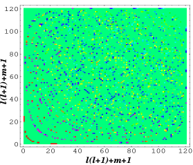
Figure 1: BipoSH coefficients are linear combinations of elements of the covariance matrix. Here $A^{2M}_{ll^{\prime}}$ (left) and $A^{4M}_{ll^{\prime}}$ (right) are plotted to show how BiPS covers the off-diagonal elements of the covariance matrix in harmonic space.

This means that $A^{\ell M}_{l_{1}l_{2}}$ completely represent the information of the covariance matrix. Fig. 1 shows how $A^{2M}_{l_{1}l_{2}}$ and $A^{4M}_{l_{1}l_{2}}$ combine the elements of the covariance matrix. When SI holds, the covariance matrix is diagonal and hence

$$A_{ll^{\prime}}^{\ell M}\, = \,(-1)^{l}C_{l}(2l+1)^{1/2}\,\delta_{ll^{\prime}}\,\delta_{\ell 0}\,\delta_{M0},$$ (23)

$$A^{00}_{l_{1}l_{2}}\, = \,(-1)^{l_{1}}\sqrt{2l_{1}+1}\,C_{l_{1}}\,\delta_{l_{1}l_{2}}.$$

BipoSH expansion is the most general way of studying two point correlation functions of CMB anisotropy. The well known angular power spectrum, $C_{l}$ is in fact a subset of BipoSH coefficients.

It is impossible to measure all $A^{\ell M}_{l_{1}l_{2}}$ individually because of cosmic variance. Combining BipoSH coefficients into Bipolar Power Spectrum reduces the cosmic variance. BiPS of CMB anisotropy is defined as a convenient contraction of the BipoSH coefficients

$$\kappa_{\ell}\,=\,\sum_{l,l^{\prime},M}|A_{ll^{\prime}}^{\ell M}|^{2}\geq 0.$$ (24)

The BiPS has interesting properties. It is orientation independent and is invariant under rotations of the sky. For models in which statistical isotropy is valid, BipoSH coefficients are given by eqn (23). And results in a null BiPS, i.e. $\kappa_{\ell}\,=\,0$ for every positive $\ell$,

$$\kappa_{\ell}\,=\,\kappa_{0}\delta_{\ell 0}.$$ (25)

So, non-zero components of BiPS imply the break down of statistical isotropy. And this introduces BiPS as a measure of statistical isotropy.

$${\mathrm{\Huge STATISTICAL\,\,\,\,ISOTROPY}}\,\,\,\,\,\,\,\Longrightarrow\,\,\,\,\,\,\,\kappa_{\ell}\,=\,0\,\,\,\,\,\,\,\forall\ell\neq 0.$$ (26)

3 BiPS Representation in Real Space

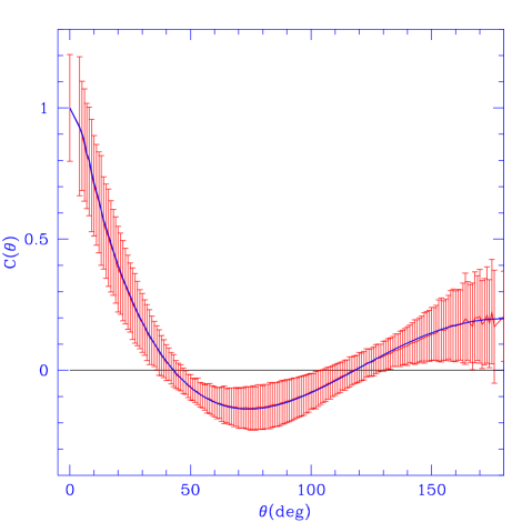
Figure 2: $C(\theta)$ ‘recovered’ from a map of a statistically isotropic model matches the original $C(\theta)$ shown as a solid line from which we made the map. The error bars shown are computed from 10 realizations. Note that the size of error bar depends on the size of $\theta$ bins.

Two point correlation of the CMB anisotropy is given by ensemble average over many universes (eqn.(6)). But in reality, there is only one universe and the ensemble average is meaningless unless the CMB sky is SI, where the two point correlation function $C(\theta)$ can be well estimated by the average product of temperature fluctuations in two directions $\hat{n}$ and $\hat{n}^{\prime}$ whose angular separation is $\theta$ (see Fig. 2), this can be written as

$$\tilde{C}(\theta)\,=\int{\frac{\mathrm{d}\Omega_{\hat{n}}}{4\pi}\int{\frac{\mathrm{d}\Omega_{\hat{n}^{\prime}}}{4\pi}\delta(\hat{n}\cdot\hat{n}^{\prime}-\cos{\theta})\Delta T(\hat{n})\Delta T(\hat{n}^{\prime})}}$$ (27)

If the statistical isotropy is violated the estimate of the correlation function from a sky map given by a single temperature product

$$\tilde{C}(\hat{n}_{1},\hat{n}_{2})\,=\,\Delta T(\hat{n}_{1})\Delta T(\hat{n}_{2})$$ (28)

is poorly determined.

Although it is not possible to estimate each element of the full correlation function $C(\hat{n}_{1},\hat{n}_{2})$, some measures of statistical isotropy of the CMB map can be estimated through suitably weighted angular averages of $\Delta T(\hat{n}_{1})\Delta T(\hat{n}_{2})$. The angular averaging procedure should be such that the measure involves averaging over sufficient number of independent measurements , but should ensure that the averaging does not erase all the signature of statistical anisotropy. Another important desirable property is that measure be independent of the overall orientation of the sky. Based on these considerations, we have proposed a set of measures of statistical isotropy Hajian & Souradeep 2003b which can be shown that is equivalent to the one in eqn.(24)

$$\kappa^{\ell}\,=\,(2l+1)^{2}\int d\Omega_{n_{1}}\int d\Omega_{n_{2}}\,[\frac{1}{8\pi^{2}}\int d{\mathcal{R}}\chi^{\ell}({\mathcal{R}})\,C({\mathcal{R}}\hat{n}_{1},\,{\mathcal{R}}\hat{n}_{2})]^{2}.$$ (29)

In the above expression, $C({\mathcal{R}}\hat{n}_{1},\,{\mathcal{R}}\hat{n}_{2})$ is the two point correlation at ${\mathcal{R}}\hat{n}_{1}\,$ and ${\mathcal{R}}\hat{n}_{2}$ which are the coordinates of the two pixels $\hat{n}_{1}\,$ and $\hat{n}_{2}$ after rotating the coordinate system through an angle $\omega$ where $(0\leq\omega\leq\pi)$ about the axis ${\bf n}(\Theta,\Phi)$. The direction of this rotation axis ${\bf n}$ is defined by the polar angles $\Theta$ where $(0\leq\Theta\leq\pi)$ and $\Phi$, where $(0\leq\Phi\leq 2\pi)$. $\chi^{\ell}$ is the trace of the finite rotation matrix in the $\ell M$-representation

$$\chi^{\ell}({\mathcal{R}})\,=\,\sum_{M=-\ell}^{\ell}D_{MM}^{\ell}({\mathcal{R}}),$$ (30)

which is called the characteristic function, or the character of the irreducible representation of rank $\ell$. It is invariant under rotations of the coordinate systems. Explicit forms of $\chi^{\ell}({\mathcal{R}})$ are simple when ${\mathcal{R}}$ is specified by $\omega,\,\Theta,\,\Phi$, then $\chi^{\ell}({\mathcal{R}})$ is completely determined by the rotation angle $\omega$ and it is independent of the rotation axis ${\bf n}(\Theta,\Phi)$,

$$\chi^{\ell}({\mathcal{R}})\, = \,\chi^{\ell}(\omega)\,$$

$$= \,\frac{\sin{[(2\ell+1)\omega/2]}}{\sin{[\omega/2]}}\,\,.$$

And finally $d{\mathcal{R}}$ in eqn(29) is the volume element of the three-dimensional rotation group and is given by

$$d{\mathcal{R}}\,=\,4\,\sin^{2}{\omega\over{2}}\,d\omega\,\sin{\Theta}\,d\Theta\,d\Phi\,\,.$$ (32)

As it is shown in Appendix (D), this expression for BiPS may be simplified further as

$$\kappa_{\ell}\,=\,\frac{2\ell+1}{8\pi^{2}}\int d\Omega_{1}\int d\Omega_{2}C(\hat{q}_{1},\hat{q}_{2})\int dR\chi_{\ell}(R)C(R\hat{q}_{1},R\hat{q}_{2})$$ (33)

For a statistically isotropic model $C(\hat{n}_{1},\,\hat{n}_{2})$ is invariant under rotation, and therefor $C({\mathcal{R}}\hat{n}_{1},\,{\mathcal{R}}\hat{n}_{2})\,=\,C(\hat{n}_{1},\,\hat{n}_{2})$. If we use this property to substitute in eqn.(33) for $C({\mathcal{R}}\hat{n}_{1},\,{\mathcal{R}}\hat{n}_{2})$, and if we use the orthonormality of $\chi^{\ell}(\omega)$ (see eqn. F7), we will recover the condition for SI,

$$\kappa^{\ell}\,=\,\kappa^{0}\delta_{\ell 0}.$$ (34)

The proof of equivalence of BiPS definition in eqns.(29) and (24) is as follows. In eqn.(29), we substitute (30) for $\chi^{\ell}({\mathcal{R}})$ and from

$$C({\mathcal{R}}\hat{n}_{1},\,{\mathcal{R}}\hat{n}_{2})\,=\,\sum_{l_{1}l_{2}}^{\ell M^{\prime}}A_{l_{1}l_{2}}^{\ell M^{\prime}}\sum_{M}D_{MM^{\prime}}^{\ell}({\mathcal{R}})\{Y_{l_{1}}(\hat{n}_{1})\otimes Y_{l_{2}}(\hat{n}_{2})\}_{\ell M},$$ (35)

we substitute for $C({\mathcal{R}}\hat{n}_{1},\,{\mathcal{R}}\hat{n}_{2})$ and use the orthonormality of $D_{MM}^{\ell}({\mathcal{R}})$ (see eqn.(F8)), we will obtain the eq.(24). Real-space representation of BiPS is very suitable for analytical compution of BiPS for theoretical models where we know the analytical expression for the two point correlation of the model, such as theoretical models in Hajian & Souradeep 2003a . This formalism would immensely simplify analytical calculations. On the other hand, the harmonic representation of BiPS allows computationally rapid methods for BiPS estimation from a given CMB map.

4 Unbiased Estimator of BiPS

In statistics, an estimator is a function of the known data that is used to estimate an unknown parameter; an estimate is the result from the actual application of the function to a particular set of data. Many different estimators may be possible for any given parameter. The above theory can be use to construct an estimator for measuring BipoSH coefficients from a given CMB map

$$\tilde{A}_{ll^{\prime}}^{\ell M}=\sum_{mm^{\prime}}\sqrt{W_{l}W_{l^{\prime}}}a_{lm}a_{l^{\prime}m^{\prime}}\,\,{\mathcal{C}}^{\ell M}_{lml^{\prime}m^{\prime}}\,\quad,$$ (36)

where $W_{l}$ is the Legendre transform of the window function. The above estimator is un-biased. Bias is the mismatch between ensemble average of the estimator and the true value. Bias for the BiPS is defined as ${\mathfrak{B}}_{\ell}=\langle\tilde{\kappa}_{\ell}\rangle-\kappa_{\ell}$ and is equal to

$${\mathfrak{B}}_{\ell}=\sum_{l_{1},l_{2}}W_{l_{1}}W_{l_{2}}\,\,\sum_{m_{1},m_{1}^{\prime}}\sum_{m_{2},m_{2}^{\prime}} \,\left[\langle a^{*}_{l_{1}m_{1}}a_{l_{1}m_{1}^{\prime}}\rangle\langle a^{*}_{l_{2}m_{2}}a_{l_{2}m_{2}^{\prime}}\rangle+\langle a^{*}_{l_{1}m_{1}}a_{l_{2}m_{2}^{\prime}}\rangle\langle a^{*}_{l_{2}m_{2}}a_{l_{1}m_{1}^{\prime}}\rangle\right]$$ (37)

$${}\times\sum_{M}\mathcal{C}^{\ell M}_{l_{1}m_{1}l_{2}m_{2}}\mathcal{C}^{\ell M}_{l_{1}m_{1}^{\prime}l_{2}m_{2}^{\prime}}\,.$$

Therefore an un-biased estimator of BiPS is given by

$$\tilde{\kappa}_{\ell}=\sum_{ll^{\prime}M}\left|\tilde{A}_{ll^{\prime}}^{\ell M}\right|^{2}-{\mathfrak{B}}_{\ell}\,,$$ (38)

The above expression for ${\mathfrak{B}}_{\ell}$ is obtained by assuming Gaussian statistics of the temperature fluctuations. The procedure is very similar to computing cosmic variance (which is discussed in the next section), but much simpler. However, we can not measure the ensemble average in the above expression and as a result, elements of the covariance matrix (obtained from a single map) are poorly determined due to the cosmic variance. The best we can do is to compute the bias for the SI component of a map

$${\mathfrak{B}}_{\ell}\equiv\langle\tilde{\kappa}_{\ell}^{B}\rangle_{{}_{\rm SI}}=(2\ell+1)\,\sum_{l_{1}}\sum_{l_{2}=|\ell-l_{1}|}^{\ell+l_{1}}C_{l_{1}}C_{l_{2}}W_{l_{1}}W_{l_{2}}\left[1+(-1)^{\ell}\,\delta_{l_{1}l_{2}}\right]\,.$$ (39)

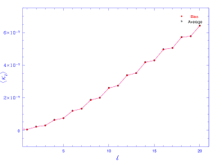
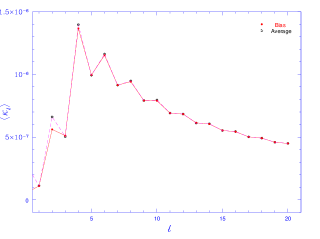
Figure 3: Analytical bias for (left) a two beam window function with $W_{l}^{S}(20,30)$ and (right) a Gaussian window function with $W_{l}^{G}(40)$ computed from the average $C_{l}$ from 1000 realizations of a SI CMB map compared with $\langle\kappa_{l}^{realization}\rangle$ (the average $\kappa_{l}$ from 1000 realizations). This shows that the theoretical bias is a very good estimation of the bias for a statistically isotropic map.

Note , the estimator $\tilde{\kappa}_{\ell}$ is unbiased, only for SI correlation,i.e., $\langle\tilde{\kappa}_{\ell}\rangle=0$. Consequently, for SI correlation, the measured $\tilde{\kappa}_{\ell}$ will be consistent with zero within the error bars given by $\sigma_{{}_{\rm SI}}$ Hajian & Souradeep 2003b . We simulated 1000 SI CMB maps and computed BiPS for them using different filters. The average BiPS of SI maps is an estimation of the bias which can be compared to our analytical estimation. Fig. 3 shows that the theoretical bias (computed from average $C_{l}$) match the numerical estimations of average $\kappa_{\ell}$ of the 1000 realizations of the SI maps.

It is important to note that bias cannot be correctly subtracted for non-SI maps. Non-zero $\tilde{\kappa}_{\ell}$ estimated from a non-SI map will have contribution from the non-SI terms in full bias given in eq. (37). It is not inconceivable that for strong SI violation, ${\mathfrak{B}}_{\ell}$ over-corrects for the bias leading to negative values of $\tilde{\kappa}_{\ell}$. What is important is whether measured $\tilde{\kappa}_{\ell}$ differs from zero at a statistically significant level.

5 Cosmic Variance

Cosmic variance is defined as the variance of the estimator of the BiPS

$$\sigma^{2}\,=\,<\tilde{\kappa}_{\ell}^{2}>-<\tilde{\kappa}_{\ell}>^{2}$$ (40)

We can analytically compute the variance of $\tilde{\kappa}^{\ell}$ using the Gaussianity of $\Delta T$. Looking back at the eq.(29) we can see, we will have to calculate the eighth moment of the field

$$\langle\Delta T(\hat{n}_{1})\Delta T(\hat{n}_{2})\Delta T(\hat{n}_{3})\Delta T(\hat{n}_{4})\Delta T(\hat{n}_{5})\Delta T(\hat{n}_{6})\Delta T(\hat{n}_{7})\Delta T(\hat{n}_{8})\rangle.$$ (41)

Assuming Gaussianity of the field we can rewrite the eight point correlation in terms of two point correlations. One can write a simple code to do that. This will give us $(8-1)!!=7\times 5\times 3=105$ terms. These 105 terms consist of terms like:

$$\langle\Delta T(\hat{n}_{1})\Delta T(\hat{n}_{2})\rangle\langle\Delta T(\hat{n}_{3})\Delta T(\hat{n}_{4})\rangle\langle\Delta T(\hat{n}_{5})\Delta T(\hat{n}_{6})\rangle\langle\Delta T(\hat{n}_{7})\Delta T(\hat{n}_{8})\rangle,$$ (42)

and all other permutations of them. On the other hand $\langle\tilde{\kappa}_{\ell}\rangle$ has a 4 point correlation in it which can also be expanded versus two point correlation functions. If we form $\langle\tilde{\kappa}_{\ell}^{2}\rangle-\langle\tilde{\kappa}_{\ell}\rangle^{2}$, only 96 terms will be left which are in the following form

$$(\frac{2\ell+1}{8\pi^{2}})^{2}\int d\Omega_{1}\cdots d\Omega_{4}\int dR\int dR^{\prime}\chi_{\ell}(R)\chi_{\ell}(R^{\prime})C(\hat{n}_{1},R^{\prime}\hat{n}_{4})C(\hat{n}_{2},R^{\prime}\hat{n}_{3})C(R\hat{n}_{1},\hat{n}_{4})C(R\hat{n}_{2},\hat{n}_{3})$$ (43)

and all other permutations. In Appendix E we explain how we can handle these 96 terms to compute the following analytical expression for cosmic variance

$$\sigma^{2}_{{}_{\rm SI}}(\tilde{\kappa}_{\ell})=\sum_{l:2l\geq\ell}\!\!4\,C_{l}^{4}W_{l}^{4}\left[2\frac{(2\ell+1)^{2}}{2l+1}+(-1)^{\ell}(2\ell+1)+(1+2(-1)^{\ell})F_{ll}^{\ell}\right]$$

$${}+\sum_{l_{1}}\sum_{l_{2}=|\ell-l_{1}|}^{\ell+l_{1}}\!\!\!4\,C_{l_{1}}^{2}\,C_{l_{2}}^{2}W_{l_{1}}^{2}\,W_{l_{2}}^{2}\left[(2\ell+1)+F_{l_{1}l_{2}}^{\ell}\right]$$

$$+\,8\sum_{l_{1}}\,\frac{(2\ell+1)^{2}}{2l_{1}+1}\,C_{l_{1}}^{2}W_{l_{1}}^{2}\left[\sum_{l_{2}=|\ell-l_{1}|}^{\ell+l_{1}}C_{l_{2}}W_{l_{2}}\right]^{2}$$

$${}+16\,(-1)^{\ell}\,\sum_{l_{1}:2l_{1}\geq\ell}\,\frac{(2\ell+1)^{2}}{2l_{1}+1}\,\sum_{l_{2}=|\ell-l_{1}|}^{\ell+l_{1}}C_{l_{1}}^{3}C_{l_{2}}\,W_{l_{1}}^{3}W_{l_{2}}.$$ (44)

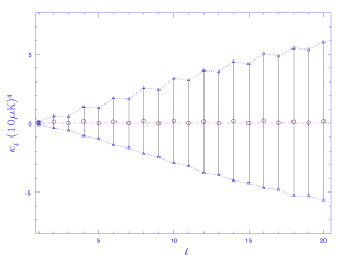
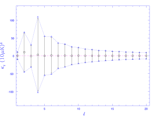
Figure 4: Bias corrected ‘measurement’ of BiPS, $\tilde{\kappa_{\ell}}$ for SI CMB maps with a best fit LCDM power spectrum smoothed by (left:) a two beam function $W_{l}^{S}(20,30)$ and (right:) a Gaussian beam $W_{l}^{G}(40)$. The cosmic error, $\sigma({\kappa_{\ell}})$, obtained using $1000$ independent realizations of CMB (full) sky map matches the analytical results shown by dotted curve with triangles . This shows a much better fit to the theoretical cosmic variance compared to what was obtained for $100$ realizations Hajian & Souradeep 2003b

Numerical computation of $\sigma^{2}_{{}_{\rm SI}}$ is fast. But the challenge is to compute Clebsch-Gordan coefficients for large quantum numbers. We use drc3j subroutine of netlib in order to compute the Clebsch-Gordan coefficients in our codes. Again we can check the accuracy of our analytical estimation of cosmic variance by comparing it against the standard deviation of BiPS of 1000 simulations of SI CMB sky. The result is shown in Fig. 4 and shows a very good agreement between the two.

6 Sources of Breakdown of Statistical Isotropy

An observed map of CMB anisotropy, $\Delta T^{obs}(\hat{n})$, is an $n$-dimensional vector ($n=12\,\times\,512^{2}$ for the WMAP data at HEALPix resolution $N_{\mathrm{s}ide}=512$). This observed map contains the true CMB temperature fluctuations, $\Delta T(\hat{n})$, convolved with the beam and buried into noise and foreground contaminations. The observed map is related to the true map through this relation

$${\mathbf{\Delta}T^{obs}}\,=\,B{\mathbf{\Delta}T}\,+\,\mathbf{n},$$ (45)

in which $B$ is a matrix that contains the information about the beam smoothing effect and $\mathbf{n}$ is the contribution from instrumental noise and foreground contamination. Hence, the observed map is a realization of a Gaussian process with covariance $C=C^{T}+C^{N}+C^{res}$ where $C^{T}$ is the theoretical covariance of the CMB temperature fluctuations, $C^{N}$ is the noise covariance matrix and $C^{res}$ is the covariance of residuals of foregrounds. Breakdown of statistical isotropy can occur in any of these parts. In general we can divide these effects into two kinds:

• Theoretical effects: These effects are theoretically motivated and are intrinsic to the true CMB sky, ${\Delta T}$. We discuss two examples of these effects, i.e. non-trivial cosmic topology and primordial magnetic fields, in the next sections.

• Observational artifacts: In an ideally cleaned CMB map, the true CMB temperature fluctuations are completely extracted from the observed map. But this is not always true. Sometimes there are some artifacts (related to $B$ or $\mathbf{n}$) left in the cleaned map which may in principle violate the SI. These effects are explained in section 6.3.

6.1 Signatures of Cosmic Topology

The question of size and the shape of our universe are very old problems that have received increasing attention over the past few years Ellis (1971); Lachieze-Rey & Luminet (1995); Levin et al. (1998); Bond,Pogosyan & Souradeep 1998, (2000); de Oliveira-Costa et al. (2003, 1996); Dineen et al. (2004); Copi et al. (2004). Although a multiply connected universe sounds non-trivial, but there are theoretical motivations Linde (2004); Levin (2002) to favor a spatially compact universe. One possibility to have a compact flat universe is the consideration of multiply connected (topologically nontrivial) spaces. The oldest way of searching for global structure of the universe is by identifying ghost images of local galaxies and clusters or quasars at higher redshifts Lachieze-Rey & Luminet (1995). This method can probe the topology of the universe only on scales substantially smaller than the apparent radius of the observable universe. Another method to search for the shape of the universe is through the effect on the power spectrum of cosmic density perturbation fields. In principle, this effect can be observed in the distribution of matter in the universe and the CMB anisotropy. Over the past few years, many independent methods have been proposed to search for evidence of a finite universe in CMB maps. These methods can be classified in three main groups.

• Using the angular power spectrum of CMB anisotropies to probe the topology of the Universe. The angular power spectrum, however, is inadequate to characterize the peculiar form of the anisotropy manifest in small universes of this type. It has been shown that a nontrivial topology breaks the SI down and as a result, there is more information in a map of temperature fluctuations than just the angular power spectrum Levin et al. (1998); Bond,Pogosyan & Souradeep 1998, (2000); Hajian & Souradeep 2003a .

• The second class of methods are direct methods which rely on multiple imaging of the CMB sky. The most well known methods amongst these methods are S-map statistics de Oliveira-Costa et al. (1996, 2003) and the search for circles-in-the-sky Cornish,Spergel & Starkman (1998).

• Third class of methods are indirect probes which deal with the correlation patterns of the CMB anisotropy field by using an appropriate combination of coefficients of the harmonic expansion of the field Dineen et al. (2004); Donoghue et al. (2004); Hajian & Souradeep 2003a ; Copi et al. (2004).

The BiPS method is one of the strategies for detecting observable signatures of a small compact universe. The BiPS method is essentially based on the search for correlation patterns in CMB. Using the fact that statistical isotropy is violated in compact spaces one could use the bipolar power spectrum as a probe to detect the topology of the universe. A simple example of application of BiPS in constraining topology of the universe is for a $T^{3}$ universe, where the correlation function is given by

$$C({\hat{q},\hat{q}^{\prime}})=L^{-3}\sum_{{\bf n}}P_{\Phi}(k_{\bf n})\,\,{\mathrm{e}}^{-i\pi(\epsilon_{\hat{q}}{\bf n}\cdot{\hat{q}}-\epsilon_{\hat{q}^{\prime}}{\bf n}\cdot{\hat{q}}^{\prime})},$$ (46)

in which, ${\bf n}$ is 3-tuple of integers (in order to avoid confusion, we use $\hat{q}$ to represent the direction instead of $\hat{n}$), the small parameter $\epsilon_{\hat{q}}\leq 1$ is the physical distance to the SLS along $\hat{q}$ in units of $L/2$ (more generally, $\bar{L}/2$ where $\bar{L}=(L_{1}L_{2}L_{3})^{1/3}$) and $L$ is the size of the Dirichlet domain (DD). When $\epsilon$ is a small constant, the leading order terms in the correlation function eq. (46) can be readily obtained in power series expansion in powers of $\epsilon$. For the lowest wavenumbers $|{\mathbf{n}}|^{2}=1$ in a cuboid torus

$$C({\hat{q},\hat{q}^{\prime}}) \approx 2\sum_{i}P_{\Phi}({2\pi}/{L_{i}})\cos(\pi\epsilon\beta_{i}\Delta q_{i})$$

$$\approx C_{0}\left[1-\epsilon^{2}\,|{\mathbf{\Delta}q}|^{2}+3\,\epsilon^{4}\,\sum_{i=1}^{3}(\Delta q_{i})^{4}\right],$$

where $\Delta q_{i}$ are the components of ${\mathbf{\Delta}q}=\hat{q}-\hat{q}^{\prime}$ along the three axes of the torus and $\beta_{i}=\bar{L}/L_{i}$. From this, the non-zero $\kappa_{\ell}$ can be analytically computed to be

$$\frac{\kappa_{0}}{C_{0}^{2}}\, = \,\pi^{2}(1-4\epsilon^{2}+\frac{368}{15}\epsilon^{4}-\frac{288}{5}\epsilon^{6}+\frac{20736}{125}\epsilon^{8})$$

$$\frac{\kappa_{4}}{C_{0}^{2}}\, = \,\frac{12288\pi^{2}}{875}\epsilon^{8}$$ (48)

$\kappa_{4}$ has the information of the relative size of the Dirichlet domain and one can use it to constrain the topology of the universe. A detailed description of determining the topology of the universe with BiPS is given in Hajian & Souradeep 2003a .

When CMB anisotropy is multiply imaged, the bipolar power spectrum corresponds to a correlation pattern of matched pairs of circles. Since it is orientation independent, the BiPS has to be computed only once for the CMB map irrespective of the orientation of the DD with respect to the sky. This method is very fast because there are fast spherical harmonic transform methods of the CMB sky maps. Using these methods it is very fast and efficient to compute the BiPS even for maps in WMAP resolution (HEALPix, $N_{side}=512$) in a few minutes on a single processor. We have used BiPS to put constraints on the topology of the Universe. The results are in preparation and will be reported soonHajian et al. (2004).

The $A^{\ell M}_{l_{1}l_{2}}$ signature, which is not discussed here, contains more details of orientation of the SI violation. It may be possible to detect the $A^{\ell M}_{l_{1}l_{2}}$ too for strong violation of SI.

6.2 Primordial Magnetic Fields

It has been shown that a cosmological magnetic field, generated during an early epoch of inflation Ratra (1992); Bamba et al. (2004), can generate CMB anisotropies Durrer et al. (1998). The presence of a preferred direction due to a homogeneous magnetic field background leads to non-zero off-diagonal elements in the covariance matrix Chen et al. (2004). This induces correlations between $a_{l+1,m}$ and $a_{l-1,m}$ multipole coefficients of the CMB temperature anisotropy field in the following manner

$$\langle a_{lm}a^{*}_{l^{\prime}m^{\prime}}\rangle\,=\,\delta_{m,m^{\prime}}[\delta_{l,l^{\prime}}C_{l}+(\delta_{l+1,l^{\prime}-1}+\delta_{l-1,l^{\prime}+1}D_{l})],$$ (49)

where $D_{l}$ is the power spectrum of off-diagonal elements of the covariance matrix. For a Harrison-Peebles-Yu-Zel’dovich scale-invariant spectrum, $D_{l}$ behaves as $l^{-2}$. More precisely, it is given by

$$D_{l}\,=\,4\times 10^{-16}l^{-2}(\frac{B}{1nG})^{4}.$$ (50)

This clearly violates the statistical isotropy. If we substitute the above $\langle a_{lm}a^{*}_{l^{\prime}m^{\prime}}\rangle$ into eqn. (22), we will get

$$A_{l_{1}l_{2}}^{{\ell}M} \,=\, \delta_{M,0}[(-1)^{l_{1}}\sqrt{(}2l_{1}+1)C_{l_{1}}\delta_{l_{1},l_{2}}\delta_{\ell,0}$$

$$\,+\, D_{l_{1}}\sum_{m1=-l1,l1}(-1)^{m_{1}}C_{l_{1}m_{1}l_{2}-m_{1}}^{{\ell}M}\delta_{l_{1+1},l_{2-1}}$$

$$\,+\, D_{l_{1}}\sum_{m1=-l1,l1}(-1)^{m_{1}}C_{l_{1}m_{1}l_{2}-m_{1}}^{{\ell}M}\delta_{l_{1-1},l_{2+1}}].$$

The first line is the statistically isotropic part and it just contributes to $\kappa_{0}$. But the interesting parts are the two other lines. We can substitute this expression into eqn. (24) and compute the BiPS predictions for magnetic fields. This work is still under process and will be reported in the near future Hajian et al. 2004b .

6.3 Observational Artifacts

Foregrounds and observational artifacts (such as non-circular beam, incomplete/non-uniform sky coverage and anisotropic noise) would also manifest themselves as violations of SI.

• Anisotropic noise : The CMB temperature measured by an instrument is a linear sum of the cosmological signal as well as instrumental noise. The two point correlation function then has two parts, one part comes from the signal and the other one comes from the noise

  $$C(\hat{n}_{1},\,\hat{n}_{2})\,=\,C^{S}(\hat{n}_{1},\,\hat{n}_{2})\,+\,C^{N}(\hat{n}_{1},\,\hat{n}_{2}).$$ (52)

  Both signal and noise should be statistically isotropic to have a statistically isotropic CMB map. So even for a statistically isotropic signal, if the noise fails to be statistically isotropic the resultant map will turn out to be anisotropic. The noise matrix can fail to be statistically isotropic due to non-uniform coverage. Also if the noise is correlated between different pixels the noise matrix could be statistically anisotropic. A simple example of this is the diagonal (but anisotropic) noise given by the following correlation

  $$C^{N}(\hat{n},\hat{n}^{\prime})=\sigma^{2}(\hat{n})\delta_{\hat{n}\hat{n}^{\prime}}.$$ (53)

  This noise clearly violates the SI and will result a non-zero BiPS given by

  $$\kappa_{\ell}=\sum_{m=-\ell}^{\ell}{|f_{\ell m}|^{2}},$$ (54)

  where $f_{\ell m}$ are spherical harmonic transform of the noise, $f_{\ell m}=\int{\mathrm{d}\Omega_{\hat{n}}Y_{\ell m}^{*}(\hat{n})\sigma^{2}(\hat{n})}$.

• The effect of non-circular beam : In practice when we deal with data, it is necessary to take into account the instrumental response. The instrumental response is nothing but the beams width and the form of the beam and can be taken into account by defining a beam profile function $B(\hat{n},\,\hat{n}^{\prime})$. Here $\hat{n}$ denotes the direction to the center of the beam and $\hat{n}^{\prime}$ denotes the direction of the incoming photon. The temperature measured by the instrument is given by

  $$\Delta\tilde{T}(\hat{n})\,=\,\int\Delta T(\hat{n}^{\prime})B(\hat{n},\,\hat{n}^{\prime})d\Omega_{\hat{n}^{\prime}}$$ (55)

  Using this relation to calculate the correlation function $\tilde{C}(\hat{n}_{1},\,\hat{n}_{2})\,=\,\langle\Delta\tilde{T}(\hat{n}_{1})\Delta\tilde{T}(\hat{n}_{2})\rangle$ one would get

  $$\tilde{C}(\hat{n}_{1},\,\hat{n}_{2})\, = \,\int d\Omega_{\hat{n}^{\prime}}\int d\Omega_{\hat{n}^{\prime\prime}}\langle\Delta T(\hat{n}^{\prime})\Delta T(\hat{n}^{\prime\prime})\rangle B(\hat{n}_{1},\,\hat{n}^{\prime})B(\hat{n}_{2},\,\hat{n}^{\prime\prime})$$

  $$= \,\int d\Omega_{\hat{n}^{\prime}}\int d\Omega_{\hat{n}^{\prime\prime}}C(\hat{n}^{\prime},\hat{n}^{\prime\prime})B(\hat{n}_{1},\,\hat{n}^{\prime})B(\hat{n}_{2},\,\hat{n}^{\prime\prime}).$$

  Only for a circular beam where $B(\hat{n},\,\hat{n}^{\prime})\,\equiv\,B(\hat{n}\cdot\hat{n}^{\prime})$, the correlation function is statistically isotropic, $\tilde{C}(\hat{n}_{1},\,\hat{n}_{2})\,\equiv\,\tilde{C}(\hat{n}_{1}\cdot\hat{n}_{2})$. Breakdown of SI is obvious since even $C_{l}$ get mixed for a non-circular beam, $\tilde{C}_{l}=\sum_{l^{\prime}}{A_{ll^{\prime}}C_{l^{\prime}}}$ Mitra et al. (2004). Non-circularity of the beam in CMB anisotropy experiments is becoming increasingly important as experiments go for higher resolution measurements at higher sensitivity.

• Mask effects : Many experiments map only a part of the sky. Even in the best case, contamination by galactic foreground residuals make parts of the sky unusable. The incomplete sky or mask effect is another source of breakdown of SI. But, this effect can be readily modeled out. The effect of a general mask on the temperature field is as follows

  $$\Delta T^{masked}(\hat{n})\,=\,\Delta T(\hat{n})W(\hat{n}),$$ (57)

  where $W(\hat{n})$ is the mask function. One can cut different parts of the sky by choosing appropriate mask functions. Masked $a_{lm}$ coefficients can be computed from the masked temperature field,

  $$a_{lm}^{masked}\, = \,\int{\Delta T^{masked}(\hat{n})Y_{lm}^{*}(\hat{n})d\Omega_{\hat{n}}}$$

  $$= \,\sum_{l_{1}m_{1}}{a_{l_{1}m_{1}}\int{Y_{l_{1}m_{1}}(\hat{n})Y_{lm}^{*}(\hat{n})W(\hat{n})d\Omega_{\hat{n}}}}.$$

  Where $a_{l_{1}m_{1}}$ are spherical harmonic transforms of the original temperature field. We can expand $W(\hat{n})$ in spherical harmonics as well

  $$W(\hat{n})\,=\,\sum_{lm}{w_{lm}Y_{lm}(\hat{n})},$$ (59)

  and after substituting this into eqn. (• ‣ 6.3) it is seen that the masked $a_{lm}$ is given by the effect of a kernel $K_{lm}^{l_{1}m_{1}}$ on original $a_{lm}$ Prunet et al. (2004)

  $$a_{lm}^{masked}\,=\,\sum_{l_{1}m_{1}}{a_{l_{1}m_{1}}K_{lm}^{l_{1}m_{1}}}.$$ (60)

  The kernel contains the information of our mask function and is defined by

  $$K_{lm}^{l_{1}m_{1}}\, = \,\sum_{l_{2}m_{2}}{w_{l_{2}m_{2}}\int{Y_{l_{1}m_{1}}(\hat{n})Y_{l_{2}m_{2}}(\hat{n})Y_{lm}^{*}(\hat{n})d\Omega_{\hat{n}}}}$$

  $$= \,\sum_{l_{2}m_{2}}{w_{l_{2}m_{2}}\sqrt{\frac{(2l_{1}+1)(2l_{2}+1)}{4\pi(2l+1)}}C_{l_{1}0l_{2}0}^{l0}C_{l_{1}m_{1}l_{2}m_{2}}^{lm}}.$$

  In the last step of the above expression we used rule F3 of spherical harmonics to simplify the expression. The covariance matrix of a masked sky will no longer have the diagonal form of eqn.(17) because of the action of the kernel

  $$\langle a^{masked}_{lm}a^{masked\,*}_{l^{\prime}m^{\prime}}\rangle\, = \,\langle a_{l_{1}m_{1}}a^{*}_{l^{\prime}_{1}m^{\prime}_{1}}\rangle K_{lm}^{l_{1}m_{1}}K_{l^{\prime}m^{\prime}}^{l^{\prime}_{1}m^{\prime}_{1}}$$ (62)

  $$= \,C_{l_{1}}\delta_{l_{1}l^{\prime}_{1}}\delta_{m_{1}m^{\prime}_{1}}K_{lm}^{l_{1}m_{1}}K_{l^{\prime}m^{\prime}}^{l^{\prime}_{1}m^{\prime}_{1}}$$

  $$= \,\sum_{l_{1},m_{1}}{C_{l_{1}}K_{lm}^{l_{1}m_{1}}K_{l^{\prime}m^{\prime}}^{l_{1}m_{1}}}.$$

  This clearly violates the SI and results a non-zero BiPS for masked CMB skies. In the next section we apply a galactic mask to ILC map and show that signature of this mask on BiPS is a rising tail at low $\ell,(\ell<20)$.

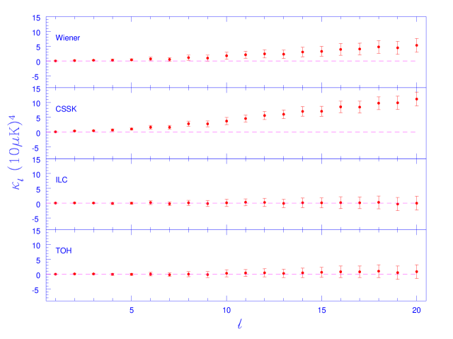
Figure 8: BiPS measured from 4 different WMAP maps filtered by $W_{l}^{S}(20,45)$. From bottom to up: TOH map, ILC map, CSSK foreground free map with a galactic cut, Wiener filtered map. We see that Wiener filtering has the similar effect as galactic cut. (But not exactly the same)

• Residuals from foreground removal : Besides the cosmological signal and instrumental noise, a CMB map also contains foreground emission such as galactic emission, etc. The foreground is usually modeled out using spectral information. However, residuals from foreground subtractions in the CMB map will violate SI. Interestingly, BiPS does sense the difference between maps with grossly different emphasis on the galactic foreground. As an example we compute BiPS of a Wiener filtered map in the next section to make this point clear (see Fig. 8). It shows a signal very similar to that of a galactic cut sky. This can be understood if one writes the effect of the Wiener filter as a weight on some regions of the map

  $$\Delta T^{W}(\hat{n})\,=\,\Delta T(\hat{n})(1+W(\hat{n})).$$ (63)

  This explains the similarity between a cut sky and a Wiener filtered map. The effect of foregrounds on BiPS still needs to be studied more carefully.

7 BiPS Results from WMAP

We carry out measurement of the BiPS, on the following CMB anisotropy maps

• a foreground cleaned map (denoted as ‘TOH’) Tegmark et al. (2004),

• the Internal Linear Combination map (denoted as ‘ILC’ in the figures) Bennett et al. (2003), and

• a customized linear combination of the QVW maps of WMAP with a galactic cut (denoted as ‘CSSK’).

Also for comparison, we measure the BiPS of

• a Wiener filtered map of WMAP data (denoted as ‘Wiener’) Tegmark et al. (2004), and

• the ILC map with a $10^{\circ}$ cut around the equator (denoted as ‘Gal. cut.’).

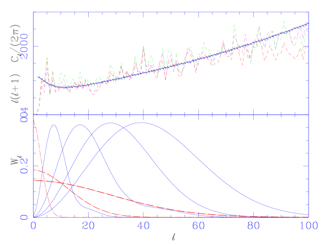
Figure 5: Top: $C_{\ell}$ of the two WMAP CMB anisotropy maps. The red, magenta and green curves correspond to map A, B and C, respectively. The black line is a ‘best fit’ WMAP theoretical $C_{\ell}$ used for simulating SI maps. Blue dots are the average $C_{l}$ recovered from $1000$ realizations. Bottom: These plots show the window functions used. The dashed curves with increasing $l$ coverage are ‘low-pass’ filter, $W_{l}^{G}(l_{s})$, with $l_{s}=4,18,40$, respectively. The solid lines are ‘band-pass’ filter $W^{S}_{l}(l_{t},l_{s})$ with $(l_{s},l_{t})=(13,2),(30,5),(30,20),(45,20)$, respectively.

Angular power spectra of these maps are shown in Fig. 5. The best fit theoretical power spectrum from the WMAP analysis   Spergel et al. (2003) is plotted on the same figure. $C_{l}$ from observed maps are consistent with the theoretical curve, $C_{l}^{T}$, (except for low multipoles. The bias and cosmic variance of BiPS depend on the total SI angular power spectrum of the signal and noise $C_{l}=C_{l}^{S}+C_{l}^{N}$. However, we have restricted our analysis to $l\mathrel{\hbox to0.0pt{\lower 4.0pt\hbox{\hskip 1.0pt$\sim$}\hss}\raise 1.0pt\hbox{$<$}}60$ where the errors in the WMAP power spectrum is dominated by cosmic variance. It is conceivable that the SI violation is limited to particular range of angular scales. Hence, multipole space windows that weigh down the contribution from the SI region of multipole space will enhance the signal relative to cosmic error, $\sigma_{{}_{\rm SI}}$. We use simple filter functions in $l$ space to isolate different ranges of angular scales; a low pass, Gaussian filter

$$W^{G}_{l}(l_{s})=\exp(-(l+1/2)^{2}/(l_{s}+1/2)^{2})$$ (64)

that cuts off power on small angular scales ($\mathrel{\hbox to0.0pt{\lower 4.0pt\hbox{\hskip 1.0pt$\sim$}\hss}\raise 1.0pt\hbox{$<$}}1/l_{s}$) and a band pass filter,

$$W^{S}_{l}(l_{t},l_{s})=\left[2(1-J_{0}((l+1/2)/(l_{t}+1/2)))\right]\,\exp(-(l+1/2)^{2}/(l_{s}+1/2)^{2})$$ (65)

that retains power within a range of multipoles set by $l_{t}$ and $l_{s}$. The windows are normalized such that $\sum_{l}(l+1/2)/(l(l+1))W_{l}=1$, i.e., unit rms for unit flat band power $C_{l}=1/(l(l+1))$. The window functions used in our work are plotted in figure 5. We use the $C_{l}^{T}$ to generate 1000 simulations of the SI CMB maps. $a_{lm}$’s are generated up to an $l_{max}$ of 1024 (corresponding to HEALPix resolution $N_{side}=512$). These are then multiplied by the window functions $W^{G}_{l}(l_{s})$ and $W^{S}_{l}(l_{t},l_{s})$. We compute the BiPS for each realization. Fig.5 shows that the average power spectrum obtained from the simulation matches the theoretical power spectrum, $C_{l}^{T}$, used to generate the realizations. We use $C_{l}^{T}$ to analytically compute bias and cosmic variance estimation for $\tilde{\kappa_{\ell}}$. This allows us to rapidly compute BiPS with $1\sigma$ error bars for different theoretical $C_{l}^{T}$.

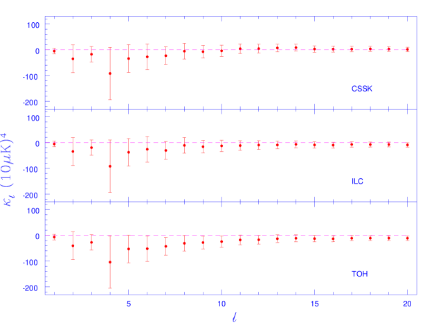
Figure 6: Figure shows the measured values of $\kappa_{\ell}$ for maps A, B and C filtered with a Gaussian window with $l_{s}=40$. Each map appears to show the violation of statistical isotropy for some $l$ at the level of $\sim 1\sigma$. However, this is because the PDF for these models are skewed with the maximum probability shifted away from the mean to negative values (see Fig. 9).

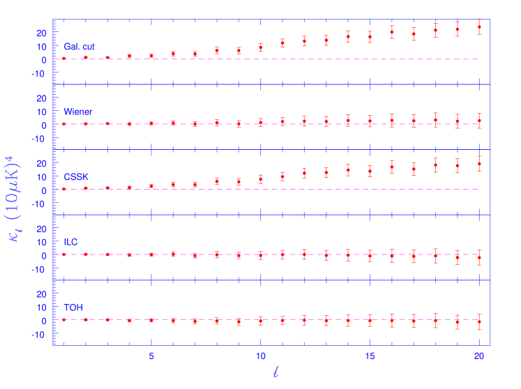
Figure 7: Measured BiPS for maps A, B and C filtered with a window with $l_{s}=30$, $l_{t}=20$. This is to check the statistical isotropy of the WMAP in the modest $20<l<40$ in the multipole space where certain anomalies have been reported. ILC with a 10-degree-cut (top) has the same BiPS as map C ($l_{s}=30$, $l_{t}=20$) which explains that the raising tail of CSSK map is because of the mask.

We use the estimator given in eqn.(36) to measure BiPS for the given CMB maps. We compute the BiPS for all window functions shown in Fig 5. Results for three of these windows are plotted in Figs. 6, 7, and 8. In the low-$l$ regime, where we have kept the low multipoles, BiPS for all three given maps are consistent with zero (Fig. 6). But in the intermediate-$l$ regime (Fig. 7), although BiPS of ILC and TOH maps are well consistent with zero, the CSSK map shows a rising tail in BiPS due to the galactic mask. To confirm it, we compute the BiPS for the ILC map with a 10-degree cut around the galactic plane (filtered with the same window function). The result is shown on the top panel of Fig. 7. Another interesting effect is seen when we apply a $W_{l}^{S}(20,45)$ filter, where Wiener filtered map has a non zero BiPS very similar to that of CSSK but weaker (Fig. 8). The reason is that Wiener filter takes out more modes from regions with more foregrounds since these are inconsistent with the theoretical model. As a result, a Wiener filtered map at $W_{l}^{s}(20,45)$ filter has a BiPS similar to a cut sky map. The fact that Wiener map has less power at the Galactic plane can even be seen by eye! Comparing Fig. 7 to Fig.8 we see that using different filters allows us to uncover different types of violation of SI in a CMB map. In our analysis we have used a set of filters which enables us to probe SI breakdown on angular scales $l\mathrel{\hbox to0.0pt{\lower 4.0pt\hbox{\hskip 1.0pt$\sim$}\hss}\raise 1.0pt\hbox{$<$}}60$.

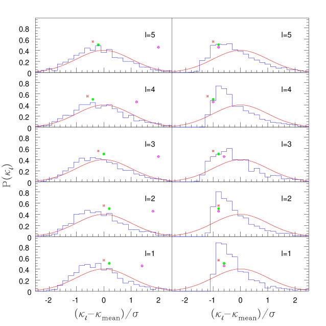
Figure 9: Probability distribution function for $\kappa_{1}$ to $\kappa_{5}$ constructed from $1000$ realizations. The left panel shows the PDF for the maps filtered with $W^{S}_{l}(20,30)$ (left panel) and $W^{G}_{l}(l_{s}=40)$ (right panel). The latter is more skewed, which explains the $\sim 1\sigma$ shift in $\kappa_{\ell}$ values shown in Fig. (6). The green, magenta and red (circular, pentagonal and rectangular) points represent ILC, CSSK and TOH maps, respectively. The smooth solid curves are Gaussian approximations.

The BiPS measured from $1000$ simulated SI realizations of $C_{l}^{T}$ is used to estimate the probability distribution functions (PDF), $p(\tilde{\kappa}_{\ell})$. A sample of the PDF for two windows is shown in Fig. 9. Measured values of BiPS for ILC, TOH and CSSK maps are plotted on the same plot. BiPS for ILC and TOH maps are located very close to the peak of the PDF. We compute the individual probabilities of the map being SI for each of the measured $\tilde{\kappa}_{\ell}$. This probability is obtained by integrating the PDF beyond the measured $\tilde{\kappa}_{\ell}$. To be precise, we compute

$$P(\tilde{\kappa}_{\ell}|{C_{l}^{T}}) = P(\kappa_{\ell}>\tilde{\kappa}_{\ell})=\int_{\tilde{\kappa}_{\ell}}^{\infty}d\kappa_{\ell}\,p(\kappa_{\ell}),\,\,\,\,\,\tilde{\kappa}_{\ell}>0,$$

$$= P(\kappa_{\ell}<\tilde{\kappa}_{\ell})=\int_{-\infty}^{\tilde{\kappa}_{\ell}}d\kappa_{\ell}\,p(\kappa_{\ell}),\,\,\,\,\,\tilde{\kappa}_{\ell}<0.$$

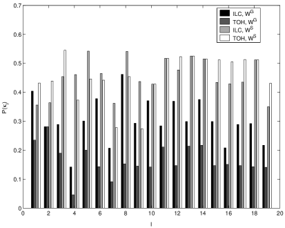
Figure 10: The probability of the two WMAP based CMB maps being SI when filtered by $W_{l}^{S}(20,30)$ and a Gaussian filter $W_{l}^{G}(40)$.

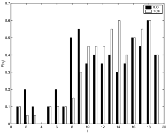
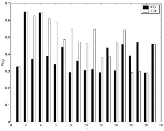
Figure 12: probability of the two WMAP based CMB maps being SI when filtered by $W_{l}^{G}(4)$ to only keep the lowest multipoles when assuming the WMAP theoretical spectrum, $C_{l}^{T}$ (left) and a model spectrum that matches the suppressed power at the lowest multipoles (right).

The probabilities obtained are shown in Figs. 10 and 12 for $W^{S}(20,30),W_{l}^{G}(40)$ and $W_{l}^{G}(4)$. The probabilities for the $W^{S}_{l}(20,30)$ window function are greater than $0.25$ and the minimum probability at $\sim 0.05$ occurs at $\kappa_{4}$ for $W^{G}(40)$. The reason for systematically lower SI probabilities for $W{{}_{l}}^{S}(20,30)$ as compared to $W{{}_{l}}^{G}(40)$ is simply due to lower cosmic variance of the former. The contribution to the cosmic variance of BiPS is dominated by the low spherical harmonic multipoles. Filters that suppress the $a_{lm}$ at low multipoles have a lower cosmic variance.

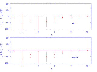
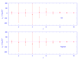
Figure 11: Figure compares the measured values of $\kappa_{\ell}$ for maps A and B filtered to retain power only on the lowest multipoles, $l=2$ and $l=3$ assuming the WMAP theoretical spectrum WMAPbf (left) and a model spectrum that matches the suppressed power at the lowest multipoles Shafieloo & Souradeep (2004). The non zero $\kappa_{\ell}$ ‘detections’ assuming the WMAP theoretical spectrum become consistent with zero for a $C_{l}^{T}$ that has power suppressed at low multipoles.

It is important to note that the above probability is a conditional probability of measured $\tilde{\kappa}_{\ell}$ being SI given the theoretical spectrum $C_{l}^{T}$ (used to estimate the bias). A final probability emerges as the Bayesian chain product with the probability of the theoretical $C_{l}^{T}$ used given data. Hence, small difference in these conditional probabilities for the two maps are perhaps not necessarily significant. Since the BiPS is close to zero, the computation of a probability marginalized over the $C_{l}^{T}$ may be possible using Gaussian (or, improved) approximation to the PDF of $\kappa_{\ell}$. The important role played by the choice of the theoretical model for the BiPS measurement is shown for a $W_{l}$ that retains power in the lowest multipoles, $l=2$ and $l=3$. Assuming $C_{l}^{T}$, there are hints of non-SI detections in the low $\ell$’s (left panel of Fig. 11). We also compute the BiPS using a $C_{l}^{T}$ for a model that accounts for suppressed quadrupole and octopole in the WMAP data Shafieloo & Souradeep (2004). The mild detections of a non zero BiPS vanish for this case (right panel of Fig. 11).

8 Discussion and Conclusion

The SI of the CMB anisotropy has been under scrutiny after the release of the first year of WMAP data. We use the BiPS which is sensitive to structures and patterns in the underlying total two-point correlation function as a statistical tool of searching for departures from SI. We carry out a BiPS analysis of WMAP full sky maps. We find no strong evidence for SI violation in the WMAP CMB anisotropy maps considered here. We have verified that our null results are consistent with measurements on simulated SI maps. The BiPS measurement reported here is a Bayesian estimate of the conditional probability of SI (for each $\kappa_{\ell}$ of the BiPS) given an underlying theoretical spectrum $C_{l}^{T}$. We point out that the excess power in the $C_{l}^{T}$ with respect to the measured $C_{l}$ from WMAP at the lowest multipoles tends to indicate mild deviations from SI. BiPS measurements are shown to be consistent with SI assuming an alternate model $C_{l}^{T}$ that is consistent with suppressed power on low multipoles. Note that it is possible to band together $\kappa_{\ell}$ measurements to tighten the error bars further. The full sky maps and the restriction to low $l<60$ (where instrumental noise is sub-dominant) permits the use of our analytical bias subtraction and error estimates. The excellent match with the results from numerical simulations is a strong verification of the numerical technique. This is an important check before using Monte-Carlo simulations in future work for computing BiPS from CMB anisotropy sky maps with a galactic mask and non uniform noise matrix.

There are strong theoretical motivations for hunting for SI violation in the CMB anisotropy. The possibility of non-trivial cosmic topology is a theoretically well motivated possibility that has also been observationally targeted Ellis (1971); Lachieze-Rey & Luminet (1995); Levin (2002); Linde (2004). The breakdown of statistical homogeneity and isotropy of cosmic perturbations is a generic feature of ultra large scale structure of the cosmos, in particular, of non trivial cosmic topology Bond,Pogosyan & Souradeep 1998, (2000). The underlying correlation patterns in the CMB anisotropy in a multiply connected universe is related to the symmetry of the Dirichlet domain. The BiPS expected in flat, toroidal models of the universe has been computed and shown to be related to the principle directions in the Dirichlet domain Hajian & Souradeep 2003a . As a tool for constraining cosmic topology, the BiPS has the advantage of being independent of the overall orientation of the Dirichlet domain with respect to the sky. Hence, the null result of BiPS can have important implication for cosmic topology. This approach complements direct search for signature of cosmic topology Cornish,Spergel & Starkman (1998); de Oliveira-Costa et al. (1996) and our results are consistent with the absence of the matched circles and the null S-map test of the WMAP CMB maps Cornish et al. (2003); de Oliveira-Costa et al. (2003). Full Bayesian likelihood comparison to the data of specific cosmic topology models is another approach that has applied to COBE-DMR data Bond,Pogosyan & Souradeep 1998, (2000). Work is in progress to carry out similar analysis on the large angle WMAP data. We defer to future publication, detailed analyzes and constraints on cosmic topology using null BiPS measurements, and the comparison to the results from complementary approaches. There are also other theoretical scenarios that predict breakdown of SI that can be probed using BiPS, e.g., primordial cosmological magnetic fields Durrer et al. (1998); Chen et al. (2004).

The null BiPS results also has implications for the observation and data analysis techniques used to create the CMB anisotropy maps. Observational artifacts such as non-circular beam, inhomogeneous noise correlation, residual stripping patterns, etc. are potential sources of SI breakdown. Our null BiPS results confirm that these artifacts do not significantly contribute to the maps studied here. Foreground residuals can also be sources of SI breakdown. The extent to which BiPS probes foreground residuals is yet to be fully studied and explored. We do not see any significant effect of the residual foregrounds in ILC and the TOH maps as it was mentioned by Eriksen et al. 2004c . This can not be necessarily called a discrepancy between the two results unless we know what should have been seen in the BiPS. The question is if the signal is strong enough and whether the effect smeared out in bipolar multipole space within our angular $l$-space window. On the other hand, the very fact that BiPS does show a strong signal for the Wiener filtered map, mean that at some level BiPS is sensitive to galactic residuals.

In summary, we study the Bipolar power spectrum (BiPS) of CMB which is a promising measure of SI. We find null measurements of the BiPS for a selection of full sky CMB anisotropy maps based on the first year of WMAP data. Our results rule out radical violation of statistical isotropy, and are consistent with null results for matched circles and the S-map tests of SI violation. Pending a more careful comparison, the results do not necessarily conflict with a number of other statistical tests, that hint at SI violation at low to modest statistical significance.

Appendix A More on Gaussianity

The temperature anisotropy at a given space-time point $({\mathbf{x}},\tau)$ can be written as a superposition of plane waves in $k$-space

$$\Delta T({\mathbf{x}},\hat{n},\tau)=\int{\mathrm{d}^{3}k\,e^{i{\mathbf{k}}\cdot{\mathbf{x}}}\,\Delta T({\mathbf{k}},\hat{n},\tau)}.$$ (A1)

As discussed in Ma & Bertschinger (1995), the dependence on $\hat{n}$ arises only through ${\mathbf{k}}\cdot\hat{n}$. Therefore $\Delta T({\mathbf{k}},\hat{n},\tau)$ may be represented as

$$\Delta T({\mathbf{k}},\hat{n},\tau)=\sum_{l=0}^{\infty}{(-i)^{l}(2l+1)\Delta T_{l}({\mathbf{k}},\tau)P_{l}({\mathbf{k}}\cdot\hat{n})}.$$ (A2)

The anisotropy coefficients $\Delta T_{l}({\mathbf{k}},\tau)$ are random variables whose amplitudes and phases depend on the initial perturbations and can be written as

$$\Delta T_{l}({\mathbf{k}},\tau)=\phi_{0}({\mathbf{k}})\Delta T_{l}(k,\tau),$$ (A3)

where $\phi_{0}({\mathbf{k}})$ is the initial potential perturbation and $\Delta T_{l}(k,\tau)$ is the photon transfer function, i.e. solution of Boltzmann equation with $\phi_{0}({\mathbf{k}})=1$. In general, $\Delta T_{l}(k,\tau)$ is given by the integral solution

$$\Delta T_{l}(\beta)=\int_{0}^{\tau_{0}}{\mathrm{d}\tau\Phi_{\beta}^{l}(\tau_{0}-\tau)S(\beta,\tau)},$$ (A4)

in which $S(\beta,\tau)$ is the source function, $\Phi_{\beta}^{l}$ is the ultra-spherical Bessel function and $\beta=k-K$, where $K=H_{0}^{2}(\Omega_{0}-1)$ is the curvature Zaldarriaga et al. (1998). In the flat case, the above expression has a very simple form

$$\Delta T(k)=\int_{0}^{\tau_{0}}{\mathrm{d}\tau\,e^{i\frac{{\mathbf{k}}\cdot\hat{n}}{k}(\tau-\tau_{0})}S(k,\tau)},$$ (A5)

and hence, the temperature anisotropies are given by

$$\Delta T({\mathbf{x}},\hat{n})=\int{\mathrm{d}^{3}k\,e^{i{\mathbf{k}}\cdot{\mathbf{x}}}\,\phi_{0}({\mathbf{k}})[\int_{0}^{\tau_{0}}{\mathrm{d}\tau\,e^{i\frac{{\mathbf{k}}\cdot\hat{n}}{k}(\tau-\tau_{0})}S(k,\tau)}]}.$$ (A6)

Equation (A6) clearly shows that Gaussian perturbations in primordial gravitational potential result a Gaussian CMB temperature anisotropy field.

Appendix B SI condition in harmonic space

We substitute the spherical harmonic coefficients, $a_{lm}$, from eqn. (8) in the covariance matrix to express it in terms of the two point correlation

$$\langle a_{lm}a^{*}_{l^{\prime}m^{\prime}}\rangle = \int{\int{\mathrm{d}\Omega_{\hat{n}}\mathrm{d}\Omega_{\hat{n}^{\prime}}Y_{lm}^{*}(\hat{n})Y_{l^{\prime}m^{\prime}}(\hat{n}^{\prime})\langle\Delta T(\hat{n})}\Delta T(\hat{n}^{\prime})}\rangle$$

$$= \int{\int{\mathrm{d}\Omega_{\hat{n}}\mathrm{d}\Omega_{\hat{n}^{\prime}}Y_{lm}^{*}(\hat{n})Y_{l^{\prime}m^{\prime}}(\hat{n}^{\prime})C(\hat{n},\hat{n}^{\prime})}}.$$

Under the condition of SI, eqn. (13), and after making use of the spherical harminc expansion of Legendre polynomials, eqn. (F6), in eqn. (14), the above expression will become

$$\langle a_{lm}a^{*}_{l^{\prime}m^{\prime}}\rangle = \int{\int{\mathrm{d}\Omega_{\hat{n}}\mathrm{d}\Omega_{\hat{n}^{\prime}}Y_{lm}^{*}(\hat{n})Y_{lm}(\hat{n}^{\prime})\sum_{l_{1}}{C_{l_{1}}\sum_{m_{1}}{Y_{l_{1}m_{1}}(\hat{n})Y_{l_{1}m_{1}}(\hat{n}^{\prime})}}}}$$

$$= \sum_{l_{1}}{C_{l_{1}}\sum_{m_{1}}{\delta_{ll_{1}}\delta_{l^{\prime}l_{1}}\delta_{mm_{1}}\delta_{m^{\prime}m_{1}}}}$$

$$= C_{l}\delta_{ll^{\prime}}\delta_{mm^{\prime}},$$

which is the SI condition in harmonic space, eqn. (17), and in the last line, the orthonormality relation of spherical harmonics, eqn. (F2) has been used.

Appendix C $A^{\ell M}_{l_{1}l_{2}}$ are linear combinations of $\langle a_{lm}a^{*}_{l^{\prime}m^{\prime}}\rangle$

The BiPoSH coefficients, $A^{\ell M}_{l_{1}l_{2}}$, are linear combinations $a_{lm}$. To see that, in the definition of two point correlation we can substitute for $\Delta T/T$ from eqn. (7), which will lead to the expansion of $C(\hat{n}_{1},\hat{n}_{2})$ in terms of spherical harmonics

$$C(\hat{n}_{1},\hat{n}_{2})\, = \,\langle\Delta T(\hat{n}_{1})\Delta T(\hat{n}_{2})\rangle$$ (C1)

$$= \,\sum_{lm}\sum_{l^{\prime}m^{\prime}}\langle a_{lm}a^{*}_{l^{\prime}m^{\prime}}\rangle Y_{lm}(\hat{n}_{1})Y^{*}_{l^{\prime}m^{\prime}}(\hat{n}_{2}).$$

This can be substituted in the definition of $A^{\ell M}_{l_{1}l_{2}}$ and eqn. (20) can be written as

$$A^{\ell M}_{l_{1}l_{2}}\, = \,\int d\Omega_{1}\int d\Omega_{2}C(\hat{n}_{1},\hat{n}_{2})\{{\boldmath{Y}}_{l_{1}}(\hat{n}_{1})\times Y_{l_{2}}(\hat{n}_{2})\}_{\ell M}^{*}$$ (C2)

$$= \,\int d\Omega_{1}\int d\Omega_{2}\sum_{lm}\sum_{l^{\prime}m^{\prime}}\langle a_{lm}a^{*}_{l^{\prime}m^{\prime}}\rangle Y_{lm}(\hat{n}_{1})Y^{*}_{l^{\prime}m^{\prime}}(\hat{n}_{2})\sum_{m_{1}m_{2}}C^{LM}_{l_{1}m_{1}l_{2}m_{2}}Y^{*}_{l_{1}m_{1}}(\hat{n}_{1})Y^{*}_{l_{2}m_{2}}(\hat{n}_{2})$$

$$= \,\int d\Omega_{1}\int d\Omega_{2}\sum_{lm}\sum_{l^{\prime}m^{\prime}}\langle a_{lm}a^{*}_{l^{\prime}m^{\prime}}\rangle Y_{lm}(\hat{n}_{1})Y^{*}_{l^{\prime}m^{\prime}}(\hat{n}_{2})\sum_{m_{1}m_{2}}C^{LM}_{l_{1}m_{1}l_{2}m_{2}}Y^{*}_{l_{1}m_{1}}(\hat{n}_{1})(-1)^{m_{2}}Y_{l_{2}-m_{2}}(\hat{n}_{2})$$

$$= \,\sum_{m_{1}m_{2}}(-1)^{m_{2}}\langle a_{l_{1}m_{1}}a^{*}_{l_{2}-m_{2}}\rangle C^{LM}_{l_{1}m_{1}l_{2}m_{2}}$$

By changing the dummy variable $m_{2}\to-m_{2}$ we will get

$$A^{\ell M}_{l_{1}l_{2}}\,=\,\sum_{m_{1}m_{2}}\langle a_{l_{1}m_{1}}a^{*}_{l_{2}m_{2}}\rangle(-1)^{m_{2}}C^{LM}_{l_{1}m_{1}l_{2}-m_{2}}.$$ (C3)

Appendix D Simplifying the real-space expression for BiPS

The BiPS in real-space is given by the following expression.

$$\kappa_{\ell}\,=\,(\frac{2\ell+1}{8\pi^{2}})^{2}\int d\Omega_{1}\int d\Omega_{2}\int dR_{1}\chi_{\ell}(R_{1})\int dR_{2}\chi_{\ell}(R_{2})C(R_{1}\hat{q}_{1},R_{1}\hat{q}_{2})C(R_{2}\hat{q}_{1},R_{2}\hat{q}_{2})$$ (D1)

Now if we change the variables in the following way

$$R_{1}\hat{q}_{1}=\hat{q}_{1}$$ (D2)

$$R_{1}\hat{q}_{2}=\hat{q}_{2}$$

We will have

$$\kappa_{\ell}\,=\,(\frac{2\ell+1}{8\pi^{2}})^{2}\int d\Omega_{1}\int d\Omega_{2}\int dR_{1}\chi_{\ell}(R_{1})\int dR_{2}\chi_{\ell}(R_{2})C(\hat{q}_{1},\hat{q}_{2})C(R_{2}R_{1}^{-1}\hat{q}_{1},R_{2}R_{1}^{-1}\hat{q}_{2}),$$ (D3)

and with

$$R=R_{2}R_{1}^{-1}$$ (D4)

we will get

$$\kappa_{\ell}\,=\,(\frac{2\ell+1}{8\pi^{2}})^{2}\int d\Omega_{1}\int d\Omega_{2}\int dR_{1}\chi_{\ell}(R_{1})\int dR\chi_{\ell}(RR_{1})C(\hat{q}_{1},\hat{q}_{2})C(R\hat{q}_{1},R\hat{q}_{2}).$$ (D5)

Using eqn. (F9) we can write

$$\int dR_{1}\chi_{\ell}(R_{1})\chi_{\ell}(RR_{1})\, = \,\sum_{m_{1}}\sum_{mm^{\prime}}\int dR_{1}D_{m_{1}m_{1}}^{*\ell}(R_{1})D_{mm^{\prime}}^{\ell}(R)D_{m^{\prime}m}^{\ell}(R_{1})$$ (D6)

$$= \,\sum_{m_{1}}\sum_{mm^{\prime}}D_{mm^{\prime}}^{\ell}(R)\frac{8\pi^{2}}{2\ell+1}\delta_{m_{1}m^{\prime}}\delta_{m_{1}m}$$

$$= \,\frac{8\pi^{2}}{2\ell+1}\sum_{m_{1}}D_{m_{1}m_{1}}^{\ell}(R)$$

$$= \,\frac{8\pi^{2}}{2\ell+1}\chi_{\ell}(R).$$

So, the $\kappa_{\ell}$ can be written in this form:

$$\kappa_{\ell}\,=\,\frac{2\ell+1}{8\pi^{2}}\int d\Omega_{1}\int d\Omega_{2}C(\hat{q}_{1},\hat{q}_{2})\int dR\chi_{\ell}(R)C(R\hat{q}_{1},R\hat{q}_{2}).$$ (D7)

Appendix E More on Cosmic Variance

The cosmic variance, $\langle\tilde{\kappa}_{\ell}^{2}\rangle-\langle\tilde{\kappa}_{\ell}\rangle^{2}$, has 96 terms similar to the one shown in eqn. (43) but with different combinations of $R$’s and $\hat{n}$’s. Among them, 40 terms contain at least one term like $C(R\hat{n}_{1},R\hat{n}_{2})$. These terms only contribute to $\kappa_{0}$ because when SI holds, $C(R\hat{n}_{1},R\hat{n}_{2})=C(\hat{n}_{1},\hat{n}_{2})$ and hence the integral in eqn. (D7) will be proportional to $\delta_{\ell 0}$, which is not in the interest of us. So, we can ignore them and we will be left with 56 terms. These terms, depending on the number of connected correlations in them, can be classified into 4 major groups:

1. One-loop terms, such as

   $$C(\hat{n}_{1},R^{\prime}\hat{n}_{3})C(\hat{n}_{3},R\hat{n}_{2})C(\hat{n}_{2},R^{\prime}\hat{n}_{4})C(\hat{n}_{4},R\hat{n}_{1}).$$ (E1)

   These terms get reduced to expressions with a $C_{l}^{4}$ factor and 4 Clebsch-Gordan coefficients (summation symbols are omitted for brevity),

   $$C_{l_{1}}^{4}C^{\ell M}_{l_{1}-m_{1}l_{1}-m_{3}}C^{\ell M}_{l_{1}m_{5}l_{1}m_{7}}C^{\ell M^{\prime}}_{l_{1}m_{7}l_{1}m_{5}}C^{\ell M^{\prime}}_{l_{1}-m_{1}l_{1}-m_{3}}.$$ (E2)

   There are 24 terms like this but with different combinations of indices.

2. Two-loop terms – type I, such as

   $$C(\hat{n}_{1},\hat{n}_{3})C(R^{\prime}\hat{n}_{3},R\hat{n}_{2})C(\hat{n}_{2},R\hat{n}_{1})C(\hat{n}_{4},R^{\prime}\hat{n_{4}}).$$ (E3)

   These terms get reduced to expressions with a $C_{l_{1}}^{3}C_{l_{2}}$ factor and 4 Clebsch-Gordan coefficients

   $$C_{l_{1}}^{3}C_{l_{7}}C^{\ell M}_{l_{1}-m_{1}l_{1}-m_{3}}C^{\ell M}_{l_{1}-m_{3}l_{1}m_{5}}C^{\ell M^{\prime}}_{l_{1}m_{1}l_{7}-m_{7}}C^{\ell M^{\prime}}_{l_{1}-m_{5}l_{7}-m_{7}}.$$ (E4)

   There are 16 terms like this but with different combinations of indices.

3. Two-loop terms – type II, such as

   $$C(\hat{n}_{1},R^{\prime}\hat{n}_{4})C(\hat{n}_{4},R\hat{n}_{1})C(\hat{n}_{2},R^{\prime}\hat{n}_{3})C(R\hat{n}_{2},\hat{n}_{3}).$$ (E5)

   These terms get reduced to expressions with a $C_{l_{1}}^{2}C_{l_{2}}^{2}$ factor and 4 Clebsch-Gordan coefficients

   $$C_{l_{1}}^{2}C_{l_{3}}^{2}C^{\ell M}_{l_{1}-m_{1}l_{3}-m_{3}}C^{\ell M}_{l_{1}m_{5}l_{3}m_{7}}C^{\ell M^{\prime}}_{l_{1}m_{5}l_{3}m_{7}}C^{\ell M^{\prime}}_{l_{1}-m_{1}l_{3}-m_{3}}.$$ (E6)

   There are 8 terms like this but with different combinations of indices.

4. Three-loop terms, such as

   $$C(\hat{n}_{1},\hat{n}_{3})C(R^{\prime}\hat{n}_{3},R\hat{n}_{1})C(\hat{n}_{2},R\hat{n}_{2})C(\hat{n}_{4},R^{\prime}\hat{n}_{4}).$$ (E7)

   These terms get reduced to expressions with a $C_{l_{1}}^{2}C_{l_{2}}C_{l_{3}}$ factor and 4 Clebsch-Gordan coefficients

   $$C_{l_{1}}^{2}C_{l_{3}}C_{l_{7}}C^{\ell M}_{l_{3}-m_{3}l_{1}-m_{1}}C^{\ell M}_{l_{3}-m_{3}l_{1}m_{5}}C^{\ell M^{\prime}}_{l_{1}m_{1}l_{7}-m_{7}}C^{\ell M^{\prime}}_{l_{1}-m_{5}l_{7}-m_{7}}.$$ (E8)

   There are 8 terms like this but with different combinations of indices.

Using symmetry properties of Clebsch-Gordan coefficients, eqn. (F10), and their summation rules, eqn. (F11), it is possible to simplify these 56 terms immensely. After tedious algebra we would obtain the final expression for the kernel of cosmic variance of the bipolar power spectrum:

$$4 \,C_{l_{1}}^{4}[2\frac{(2\ell+1)^{2}}{2l_{1}+1}+(-1)^{\ell}(2\ell+1)+(1+2(-1)^{\ell})F_{ll}^{\ell}]\,\{l_{1}l_{1}\ell\}+$$ (E9)

$$4 \,C_{l_{1}}^{2}C_{l_{2}}^{2}[(2\ell+1)+F_{l_{1}l_{2}}^{\ell}]\,\{l_{1}l_{2}\ell\}+$$

$$8 \,C_{l_{1}}^{2}C_{l_{2}}C_{l_{3}}\frac{(2\ell+1)^{2}}{2l_{1}+1}\,\{l_{1}l_{2}\ell\}\,\{l_{1}l_{3}\ell\}+$$

$$16 \,(-1)^{\ell}\,C_{l_{1}}^{3}C_{l_{3}}\frac{(2\ell+1)^{2}}{2l_{1}+1}\,\{l_{1}l_{1}\ell\}\,\{l_{1}l_{3}\ell\}$$

where the $3j$-symbol $\{l_{1}l_{2}\ell\}$ is given by

$$\{l_{1}l_{2}\ell\}=\left\{\begin{array}[]{ll}1&\textrm{if $l_{1}+l_{2}+\ell$ is integer and $|l_{1}-l_{2}|\leq\ell\leq(l_{1}+l_{2})$,}\\ 0&\textrm{otherwise,}\end{array}\right.$$

and $F_{l_{1}l_{3}}^{\ell}$ is defined as

$$F_{l_{1}l_{3}}^{\ell}=\!\!\!\!\sum_{m_{1}m_{2}=-l_{1}}^{l_{1}}\,\sum_{m_{3}m_{4}=-l_{3}}^{l_{3}}\sum_{M,M^{\prime}=-\ell}^{\ell}C^{\ell M}_{l_{1}-m_{1}l_{3}-m_{3}}C^{\ell M}_{l_{1}m_{2}l_{3}m_{4}}C^{\ell M^{\prime}}_{l_{3}m_{4}l_{1}m_{1}}C^{\ell M^{\prime}}_{l_{3}-m_{3}l_{1}-m_{2}}.$$ (E10)

This should be summed over all indices except $\ell$ to result the analytical expression for the cosmic variance given in eqn. (5).

Appendix F Useful Standard Integrals and Summation Rules

For completeness we list a set of standard integrals and summation rules which are needed in BiPS calculations. Orthonormality of spherical harmonics

$$\int d\Omega_{\hat{n}}\,Y_{\ell m}(\hat{n}) = \sqrt{4\pi}\delta_{\ell 0}\delta_{m0},$$ (F1)

$$\int d\Omega_{\hat{n}}\,Y_{l_{1}m_{1}}(\hat{n})Y_{l_{2}m_{2}}^{*}(\hat{n}) = \delta_{l_{1}l_{2}}\delta_{m_{1}m_{2}},$$ (F2)

$$\int d\Omega_{\hat{n}}Y_{l_{1}m_{1}}(\hat{n})Y_{l_{2}m_{2}}(\hat{n})Y_{\ell_{3}m_{3}}^{*}(\hat{n}) = \sqrt{\frac{(2l_{1}+1)(2l_{2}+1)}{4\pi(2\ell_{3}+1)}}C_{l_{1}0l_{2}0}^{\ell_{3}0}C_{l_{1}m_{1}l_{2}m_{2}}^{\ell_{3}m_{3}}.$$ (F3)

Symmetry property of spherical harmonics

$$Y_{lm}^{*}(\hat{n})=(-1)^{m}Y_{l-m}(\hat{n}).$$ (F5)

Spherical harmonic expansion of Legendre polynomials

$$P_{l}(\hat{n}\cdot\hat{n}^{\prime})=\frac{4\pi}{2l+1}\sum_{m=-l}^{l}{Y_{lm}^{*}(\hat{n})Y_{lm}(\hat{n}^{\prime})}.$$ (F6)

Orthonormality relation of $\chi^{\ell}(\omega)$

$$\int_{0}^{\pi}\chi^{\ell_{1}}(\omega)\chi^{\ell_{2}}(\omega)\sin^{2}{\omega\over{2}}d\omega\,=\,\frac{\pi}{2}\delta_{\ell_{1}\ell_{2}}.$$ (F7)

Orthonormality of $D_{MM}^{\ell}({\mathcal{R}})$

$$\int d{\mathcal{R}}D_{MM^{\prime}}^{*\ell}({\mathcal{R}})D_{mm^{\prime}}^{l}({\mathcal{R}})\,=\,\frac{8\pi^{2}}{2l+1}\,\delta_{l\ell}\delta_{mM}\delta_{m^{\prime}M^{\prime}},$$ (F8)

$$\sum_{mm^{\prime}}D_{mm^{\prime}}^{\ell}(R_{1})D_{m^{\prime}m}^{\ell}(R_{2})=\chi_{\ell}(R_{1}R_{2})$$ (F9)

Symmetry properties of Clebsch-Gordan coefficients

$$C_{a\alpha b\beta}^{c\gamma} = (-1)^{a+b-c}C_{b\beta a\alpha}^{c\gamma},$$ (F10)

$$C_{a\alpha b\beta}^{c\gamma} = (-1)^{a+b-c}C_{a-\alpha b-\beta}^{c-\gamma}.$$

Summation rules of Clebsch-Gordan coefficients

$$\sum_{\alpha\beta}C_{a\alpha b\beta}^{c\gamma}C_{a\alpha b\beta}^{c^{\prime}\gamma^{\prime}} = \delta_{cc^{\prime}}\delta_{\gamma\gamma^{\prime}}\{abc\}\{abc^{\prime}\}$$

$$\sum_{a\gamma}C_{a\alpha b\beta}^{c\gamma}C_{a\alpha b^{\prime}\beta^{\prime}}^{c\gamma} = \frac{2c+1}{2b+1}\delta_{bb^{\prime}}\delta_{\beta\beta^{\prime}}\{abc\}\{ab^{\prime}c\}$$

$$\sum_{c\gamma}C_{a\alpha b\beta}^{c\gamma}C_{a\alpha^{\prime}b\beta^{\prime}}^{c\gamma} = \delta_{\alpha\alpha^{\prime}}\delta_{\beta\beta^{\prime}}\{abc\}$$ (F11)

References

- Bamba et al. (2004) Bamba, K., Yokoyama, J., Phys.Rev. D69 (2004) 043507.
- Bardeen et al. (1983) Bardeen, J. M., Steinhardt, P. J. & Turner, M. S. 1983, Phys. Rev. D 28, 679.
- Bartolo et al. (2004) Bartolo, N., Komatsu, E., Matarrese, S., Riotto, A., preprint (astro-ph/0406398)
- Bennett et al. (2003) Bennett, C. L., et.al., 2003, Astrophys. J. Suppl., 148, 1.
- Bond (2004) Bond, J. R. et al. 2004, Int. J. Theor. Phys. 2004, ed. Verdaguer, E., ”The Early Universe: Confronting theory with observations” (June 21-27, 2003) (astro-ph/0406195).
- Bond,Pogosyan & Souradeep 1998, (2000) Bond, J. R., Pogosyan, D. & Souradeep,T. 1998, Class. Quant. Grav. 15, 2671; ibid. 2000, Phys. Rev. D 62,043005;2000, Phys. Rev. D 62,043006.
- Chen et al. (2004) Chen, G., Mukherjee, P., Kahniashvili, T., Ratra, B., Wang, Y., Astrophys.J. 611 (2004) 655.
- Coles (2003) Coles, P. et al. 2003, preprint (astro-ph/0310252).
- Copi et al. (2004) Copi, C. J., Huterer, D. & Starkman, G. D. 2004, Phys. Rev. D. in press, (astro-ph/0310511).
- Cornish,Spergel & Starkman (1998) Cornish, N.J., Spergel, D.N. & Starkman, G. D. 1998, Class. Quantum Grav., 15, 2657
- Cornish et al. (2003) Cornish, N. J., Spergel, D., Starkman, G. , Komatsu, E., 2004, Phys.Rev.Lett. 92, 201302.
- Cruz et al. (2004) Cruz, M., Martinez-Gonzalez, E., Vielva, P., Cayon, L., preprint (astro-ph/0405341).
- de Oliveira-Costa et al. (2003) de Oliveira-Costa, A., Tegmark, M., Zaldarriaga, M. & Hamilton, A. 2004, Phys. Rev.D69, 063516.
- de Oliveira-Costa et al. (1996) de Oliveira-Costa, A. Smoot, G. F., Starobinsky, A. A., 1996, ApJ 468, 457.
- Dineen et al. (2004) Dineen, P. , Rocha, G., Coles, P, preprint (astro-ph/0404356).
- Donoghue et al. (2004) Donoghue, E. P., and Donoghue, J. F., preprint (astro-ph/0411237).
- Durrer et al. (1998) Durrer, R., Kahniashvili, T. and Yates, A., 1998, Phys. Rev. D 58, 3004.
- Ellis (1971) Ellis, G. F. R. 1971, Gen. Rel. Grav. 2, 7.
- (19) Eriksen, H. K. et al., 2004, Astrophys. J 605, 14.
- (20) Eriksen, H. K. et al., 2004, Astrophys. J. 612, 64.
- (21) Eriksen, H. K. et al., 2004, Astrophys. J. 612, 633.
- Gaztanaga & Wagg (2003) Gaztanaga, E. & Wagg, J. 2003, Phys. Rev. D68 021302.
- Górski,Hivon & Wandelt (1999) Górski,K. M., Hivon, E., Wandelt, B. D. 1999, in ”Evolution of Large-Scale Structure”, eds. A.J. Banday, R.S. Sheth and L. Da Costa, PrintPartners Ipskamp, NL, pp. 37-42 (also astro-ph/9812350).
- Guth & Pi (1982) Guth, A. H. & Pi, S.-Y. 1982, Phys. Rev. Lett., 49, 1110.
- (25) Hajian, A. & Souradeep, T., 2003a preprint (astro-ph/0301590).
- (26) Hajian, A. and Souradeep, T., 2003b, ApJ 597, L5 (2003).
- Hajian & Souradeep (2004) Hajian, A. & Souradeep, T., 2005, ApJ 618, L63.
- Hajian et al. (2004) Hajian, A., Pogosyan, D. Souradeep, T., Contaldi, C., Bond, R., 2004 in preparation; Proc. 20th IAP Colloquium on Cosmic Microwave Background physics and observation, 2004.
- (29) Hajian, A., Chen, G., Souradeep, T., Kahniashvilli, T., Ratra, B., 2004 in preparation.
- Hansen et al. (2004) Hansen, F. K., Banday, A. J. & Gorski, K. M. 2004, preprint. (astro-ph/0404206)
- Hinshaw et al. (2003) G. Hinshaw, Astrophys. J. Suppl.,(2003) ,148, 135.
- Komatsu et al. (2003) Komatsu, E. et.al., 2003, ApJS, 148, 119.
- Kogut et al. (2003) Kogut A. et al., 2003, Astrophys. J. Suppl.,148, 161.
- Lachieze-Rey & Luminet (1995) Lachieze-Rey, M. and Luminet,J. -P. 1995, Phys. Rep. 25, 136.
- Larson & Wandelt (2004) Larson, D. L. & Wandelt, B. D. 2004, preprint, (astro-ph/0404037).
- Levin (2002) Levin, J. 2002, Phys. Rep. 365, 251.
- Levin et al. (1998) Levin J., Scannapieco E., Silk J., (1998), Class.Quant.Grav. 15, 2689.
- Linde (2004) Linde, A., (2004), JCAP 0410, 004, (astro-ph/0408164).
- Luminet et al. (2003) Luminet, J.-P. et al. 2003, Nature 425 593.
- Ma & Bertschinger (1995) Ma, C.-P., & Bertschinger, E. 1995, ApJ, 455, 7
- Mitra et al. (2004) Mitra, S., Sengupta, A., S., Souradeep, T.,preprint astro-ph/0405406
- Munshi et al. (1995) Munshi, D., Souradeep, T., and Starobinsky, A. A., (1995), Astrophys. J., 454, 552.
- Page et al. (2003) Page L. et al., 2003, Astrophys. J. Suppl.,148, 233.
- Naselsky et al. (2004) Naselsky et al, 2004, preprint, (astro-ph/0405523); ibid (astro-ph/0405181), 2003; ApJ,599,L53 and references therein.
- Park (2004) Park, C., 2004, Mon. Not. Roy. Astron. Soc. 349, 313.
- Peiris et al., (2003) Peiris H.V. et al., 2003, Astrophys. J. Suppl.,148, 213.
- Prunet et al. (2004) Prunet, S., Uzan, J., Bernardeau, F., Brunier, T., 2004, preprint (astro-ph/0406364).
- Ratra (1992) Ratra, B., (1992), Astrophys.J. 391, L1.
- Sachs and Wolfe, (1967) Sachs, R. K., and Wolfe, A. M. 1967, ApJ, 147, 73.
- Schwarz et al. (2004) Schwarz, D. J. et al., 2004, preprint (astro-ph/0403353).
- Shafieloo & Souradeep (2004) Shafieloo, A. & Souradeep, T., 2004, Phys. Rev. D, in press, (astro-ph/0312174).
- Souradeep (2000) Souradeep,T. 2000, in ‘The Universe’, eds. Dadhich, N. & Kembhavi, A., Kluwer.
- Souradeep & Hajian (2003) Souradeep, T. and Hajian, A., 2004, Pramana, 62, 793.
- Spergel et al. (2003) Spergel, D. et al., 2003, Astrophys. J. Suppl., 148, 175.
- Spergel et al. (1999) Spergel, D., and Goldberg, D. M., (1999), Phys.Rev. D59, 103001.
- Starkman (1998) Starkman, G. Class. 1998, Quantum Grav. 15, 2529.
- Starobinsky (1982) Starobinsky, A. A. 1982, Phys. Lett, 117B, 175.
- Tegmark et al. (2004) Tegmark, M., de Oliveira-Costa, A. & Hamilton, A., 2004, Phys.Rev. D68 123523.
- Varshalovich et al. (1988) Varshalovich, D. A., Moskalev, A. N., Khersonskii, V. K., 1988 Quantum Theory of Angular Momentum (World Scientific).
- Vielva et al. (2003) Vielva, P., Martinez-Gonzalez, E., Barreiro, R. B., Sanz, J. L., Cayon, L., 2003, preprint (astro-ph/0310273).
- Zaldarriaga et al. (1998) Zaldarriaga, M., Seljak, U., Bertschinger, E., 1998, Astrophys. J., 494, 491.