Influence of pump-field scattering to nonclassical-light generation in a photonic band-gap nonlinear planar waveguide

Abstract

Optical parametric process occurring in a nonlinear planar waveguide can serve as a source of light with nonclassical properties. Properties of the generated fields are substantially modified by scattering of the nonlinearly interacting fields in a photonic band-gap structure inside the waveguide. A quantum model of linear operator amplitude corrections to amplitude mean-values provides conditions for an efficient squeezed-light generation as well as generation of light with sub-Poissonian photon-number statistics. Destructive influence of phase mismatch of the nonlinear interaction can fully be compensated using a suitable photonic-band gap structure inside the waveguide. Also an increase of signal-to-noise ratio of an incident optical field can be reached in the waveguide.

I Introduction

Properties of linear photonic band-gap structures have been an object of intensive investigations in the last several years Bertolotti2001 ; Joannopoulos . The most typical characteristics of these structures are spatial localization of optical modes in confined regions of a given structure and high densities of these optical modes. Considering nonlinear materials, energy of an optical field is mainly contained in these localized modes and so a very strong and thus efficient nonlinear interaction can occur. For example, second harmonic and sub-harmonic generation in photonic band-gap structures has been an object of investigation in Scalora1997 ; Dumeige2001 . Phase-matching can be tailored in photonic band-gap structures so that fulfilment of phase-matching conditions for a given nonlinear process is reached and an efficient nonlinear process is guaranteed this way. In some cases the overlap of nonlinearly interacting optical fields and their mutual spatial phase relations determine the strength of nonlinear process and properties of light obtained in a nonlinear photonic band-gap structure.

These properties may also be suitable for the generation of light with nonclassical properties (squeezed light, light with sub-Poissonian photon-number statistics), as has been suggested in Sakoda2002 . Up to now, attention has been devoted to the generation of nonclassical light in nonlinear photonic band-gap waveguides. It has been shown that the process of second-harmonic generation in a planar nonlinear waveguide with a corrugation on the top can be used to control squeezing of the fundamental field Tricca2004a ; the corrugation reproduces a photonic band-gap structure. In Tricca2004a periodicity of the grating was selected to give rise to a longitudinal confinement of the pump field, phase matching of the nonlinear process was achieved introducing a spatial modulation of nonlinear susceptibility. Conditions for an efficient squeezed-light generation as well as generation of light with sub-Poissonian photon-number statistics have been analyzed in PerinaJr2004 for a nonlinear waveguide with optical parametric process; the photonic band-gap structure was set to assure longitudinal confinement of the down-converted fields.

In this contribution we extend the analysis given in PerinaJr2004 to account also for the pump-field longitudinal confinement. This confinement considerably changes amplitude and phase relations along the waveguide thus providing new possibilities for nonclassical-light generation. Optical fields participating in the nonlinear interaction are described using the generalized superposition of signal and noise.

A quantum derivation of the equations governing the evolution of the interacting optical fields is given in Sec. 2. In Sec. 3, conditions for squeezed-light generation are analyzed. Sec. 4 is devoted to photon-number statistics of the generated fields. Possibility to improve signal-to-noise ratio of an incident optical field is discussed in Sec. 5. Sec. 6 contains conclusions.

II Quantum description of the nonlinearly interacting fields

A quantum description of nonlinearly interacting optical modes requires the construction of an appropriate momentum operator $\hat{G}(z)$, which then determines Heisenberg equations of motion:

$$\frac{d\hat{X}}{dz}=-\frac{i}{\hbar}\left[\hat{G},\hat{X}\right];$$ (1)

$\hat{X}$ stands for an arbitrary operator, $\hbar$ is the reduced Planck constant, and $[\;,\;]$ means a commutator.

If a nonlinear interaction involves counter-propagating fields, we cannot straightforwardly assign any momentum operator $\hat{G}$ to the system of interacting optical fields. However, we can proceed as follows PerinaJr2000 . We assume the nonlinear interaction among all involved fields as if they co-propagate and write the momentum operator $\hat{G}(z)$ in the form:

$$\hat{G}(z)=\sum_{a=s_{F},i_{F},p_{F}}\hbar({\bf k}_{a})_{z}\hat{a}^{\dagger}_{a}\hat{a}_{a}+\sum_{a=s_{B},i_{B},p_{B}}\hbar({\bf k}_{a})_{z}\hat{a}^{\dagger}_{a}\hat{a}_{a}$$

$$\mbox{}+\left[\hbar K_{s}\exp(i\delta_{l}z)\hat{a}^{\dagger}_{s_{F}}\hat{a}_{s_{B}}+\hbar K_{i}\exp(i\delta_{l}z)\hat{a}^{\dagger}_{i_{F}}\hat{a}_{i_{B}}\right.$$

$$\mbox{}\left.+\hbar K_{p}\exp(2i\delta_{l}z)\hat{a}^{\dagger}_{p_{F}}\hat{a}_{p_{B}}+{\rm h.c.}\right]$$

$$\mbox{}-\left[2i\hbar K_{F}\hat{a}_{p_{F}}\hat{a}^{\dagger}_{s_{F}}\hat{a}^{\dagger}_{i_{F}}+2i\hbar K_{B}\hat{a}_{p_{B}}\hat{a}^{\dagger}_{s_{B}}\hat{a}^{\dagger}_{i_{B}}+{\rm h.c.}\right].$$

Symbol $\hat{a}_{a}$ ($\hat{a}_{a}^{\dagger}$) denotes an annihilation (creation) operator of mode $a$; $({\bf k}_{a})_{z}$ is the corresponding wave-vector of mode $a$ along $z-$axis. We consider six nonlinearly interacting optical modes in the investigated waveguide with optical parametric process; forward-propagating signal mode (denoted as $s_{F}$), backward-propagating signal mode ($s_{B}$), forward-propagating idler mode ($i_{F}$), backward-propagating idler mode ($i_{B}$), forward-propagating pump mode ($p_{F}$), and finally backward-propagating pump mode ($p_{B}$). Constants $K_{s}$, $K_{i}$, and $K_{p}$ describe a linear exchange of energy between forward- and backward-propagating signal, idler, and pump modes. This exchange of energy originates in scattering of fields in a photonic band-gap structure. Frequency $\delta_{l}$ determines periodicity of the corrugation on the top of the waveguide. Constants $K_{F}$ and $K_{B}$ stand for nonlinear coupling coefficients for forward- and backward-propagating fields. Values of these parameters are determined using simple expressions after a mode structure of the waveguide is found (see, e.g., in Yeh1988 ; Pezzetta2001 ). Scheme of the waveguide with the considered interactions among the involved optical fields is shown in Fig. 1.

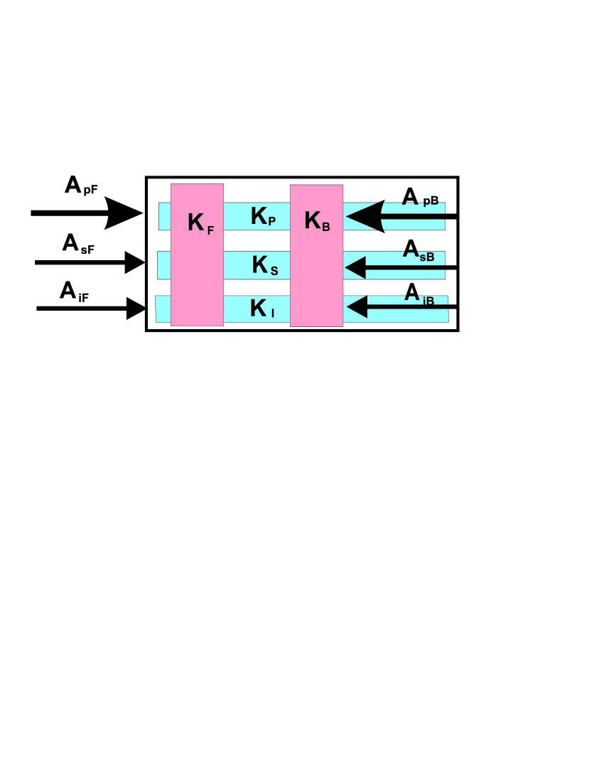
Figure 1: Scheme of the considered nonlinear planar photonic band-gap waveguide; $A_{pF}$, $A_{sF}$, and $A_{iF}$ [$A_{pB}$, $A_{sB}$, and $A_{iB}$] denote amplitudes of forward-propagating [backward-propagating] pump, signal, and idler fields; $K_{p}$, $K_{s}$, and $K_{i}$ are linear coupling constants between pump, signal, and idler fields, and $K_{F}$ ($K_{B}$) stands for a nonlinear coupling constant among forward- (backward-) propagating fields.

We now substitute creation operators ($\hat{a}^{\dagger}$) of the backward-propagating fields by newly introduced auxiliary annihilation operators ($\hat{b}$) and vice versa, i.e.

$$\hat{a}^{\dagger}_{s_{B}}\leftarrow\hat{b}_{s_{B}},\hat{a}^{\dagger}_{i_{B}}\leftarrow\hat{b}_{i_{B}},\hat{a}^{\dagger}_{p_{B}}\leftarrow\hat{b}_{p_{B}},$$

$$\hat{a}_{s_{B}}\leftarrow\hat{b}^{\dagger}_{s_{B}},\hat{a}_{i_{B}}\leftarrow\hat{b}^{\dagger}_{i_{B}},\hat{a}_{p_{B}}\leftarrow\hat{b}^{\dagger}_{p_{B}}.$$ (3)

Heisenberg equations in Eq. (1) then have the form:

$$\frac{d\hat{a}_{s_{F}}}{dz} = i({\bf k}_{s_{F}})_{z}\hat{a}_{s_{F}}+iK_{s}\exp(i\delta_{l}z)\hat{b}^{\dagger}_{s_{B}}$$

$$\mbox{}+2K_{F}\hat{a}_{p_{F}}\hat{a}^{\dagger}_{i_{F}},$$

$$\frac{d\hat{a}_{i_{F}}}{dz} = i({\bf k}_{i_{F}})_{z}\hat{a}_{i_{F}}+iK_{i}\exp(i\delta_{l}z)\hat{b}^{\dagger}_{i_{B}}$$

$$\mbox{}+2K_{F}\hat{a}_{p_{F}}\hat{a}^{\dagger}_{s_{F}},$$

$$\frac{d\hat{b}^{\dagger}_{s_{B}}}{dz} = -i({\bf k}_{s_{B}})_{z}\hat{b}^{\dagger}_{s_{B}}-iK^{*}_{s}\exp(-i\delta_{l}z)\hat{a}_{s_{F}}$$

$$\mbox{}-2K_{B}\hat{b}^{\dagger}_{p_{B}}\hat{b}_{i_{B}},$$

$$\frac{d\hat{b}^{\dagger}_{i_{B}}}{dz} = -i({\bf k}_{i_{B}})_{z}\hat{b}^{\dagger}_{i_{B}}-iK^{*}_{i}\exp(-i\delta_{l}z)\hat{a}_{i_{F}}$$

$$\mbox{}-2K_{B}\hat{b}^{\dagger}_{p_{B}}\hat{b}_{s_{B}},$$

$$\frac{d\hat{a}_{p_{F}}}{dz} = i({\bf k}_{p_{F}})_{z}\hat{a}_{p_{F}}+iK_{p}\exp(2i\delta_{l}z)\hat{b}^{\dagger}_{p_{B}}$$

$$\mbox{}-2K^{*}_{F}\hat{a}_{s_{F}}\hat{a}_{i_{F}},$$

$$\frac{d\hat{b}^{\dagger}_{p_{B}}}{dz} = -i({\bf k}_{p_{B}})_{z}\hat{b}^{\dagger}_{p_{B}}-iK_{p}^{*}\exp(-2i\delta_{l}z)\hat{a}_{p_{F}}$$ (4)

$$\mbox{}+2K^{*}_{B}\hat{b}^{\dagger}_{s_{B}}\hat{b}^{\dagger}_{i_{B}}.$$

To reach the final equations, we have to make the following steps: 1. Return to the original operators $\hat{a}^{\dagger}$, $\hat{a}$ in Eqs. (4) using the substitution in Eq. (3). 2. Transform Eqs. (4) into the interaction picture ($\hat{a}_{a}(z)=\hat{A}_{a}(z)\exp[i({\bf k}_{a})_{z}z]$). 3. Write operators $\hat{A}_{a}(z)$ in the interaction picture as $\hat{A}_{a}(z)=A_{a}(z)+\delta\hat{A}_{a}(z)$, where $A_{a}(z)$ is a classical amplitude mean-value and $\delta\hat{A}(z)$ is a small operator correction to this amplitude mean-value. This procedure results in a system of nonlinear differential equations for amplitude mean-values $A_{a}$ and a system of linear operator differential equations for small operator amplitude corrections $\delta\hat{A}_{a}$.

The system of nonlinear differential equations for classical amplitude mean-values $A_{a}$ is written as follows:

$$\frac{dA_{s_{F}}}{dz} = iK_{s}\exp(-i\delta_{s}z)A_{s_{B}}$$

$$\mbox{}+2K_{F}\exp(i\delta_{F}z)A_{p_{F}}A^{*}_{i_{F}},$$

$$\frac{dA_{i_{F}}}{dz} = iK_{i}\exp(-i\delta_{i}z)A_{i_{B}}$$

$$\mbox{}+2K_{F}\exp(i\delta_{F}z)A_{p_{F}}A^{*}_{s_{F}},$$

$$\frac{dA_{s_{B}}}{dz} = -iK^{*}_{s}\exp(i\delta_{s}z)A_{s_{F}}$$

$$\mbox{}-2K_{B}\exp(-i\delta_{B}z)A_{p_{B}}A^{*}_{i_{B}},$$

$$\frac{dA_{i_{B}}}{dz} = -iK^{*}_{i}\exp(i\delta_{i}z)A_{i_{F}}$$

$$\mbox{}-2K_{B}\exp(-i\delta_{B}z)A_{p_{B}}A^{*}_{s_{B}},$$

$$\frac{dA_{p_{F}}}{dz} = iK_{p}\exp(-i\delta_{p}z)A_{p_{B}}$$

$$\mbox{}-2K^{*}_{F}\exp(-i\delta_{F}z)A_{s_{F}}A_{i_{F}},$$

$$\frac{dA_{p_{B}}}{dz} = -iK^{*}_{p}\exp(i\delta_{p}z)A_{p_{F}}$$ (5)

$$\mbox{}+2K^{*}_{B}\exp(i\delta_{B}z)A_{s_{B}}A_{i_{B}},$$

and

$$\delta_{a} = |({\bf k}_{a_{F}})_{z}|+|({\bf k}_{a_{B}})_{z}|-\delta_{l},\hskip 14.22636pta=s,i,$$

$$\delta_{p} = |({\bf k}_{p_{F}})_{z}|+|({\bf k}_{p_{B}})_{z}|-2\delta_{l},$$

$$\delta_{b} = |({\bf k}_{p_{b}})_{z}|-|({\bf k}_{s_{b}})_{z}|-|({\bf k}_{i_{b}})_{z}|,\hskip 14.22636ptb=F,B.$$ (6)

Any solution of the system in Eqs. (5) obeys the following conservation law of energy (in quantum interpretation, “the overall number of virtual photons in the interaction” is conserved):

$$\frac{d}{dz}\left(|A_{s_{F}}|^{2}+|A_{i_{F}}|^{2}+2|A_{p_{F}}|^{2}\right.$$

$$\left.-|A_{s_{B}}|^{2}-|A_{i_{B}}|^{2}-2|A_{p_{B}}|^{2}\right)=0.$$ (7)

If the nonlinear terms in Eqs. (5) are omitted, the solution of Eqs. (5) can be written as:

$$A_{a_{F}}^{(0)} = \exp\left(-i\frac{\delta_{a}z}{2}\right)\left[B_{a}\cos(\Delta_{a}z)+\tilde{B_{a}}\sin(\Delta_{a}z)\right],$$

$$A_{a_{B}}^{(0)} = \exp\left(i\frac{\delta_{a}z}{2}\right)$$ (8)

$$\mbox{}\times\left[B_{a}\left(-\frac{\delta_{a}}{2K_{a}}\cos(\Delta_{a}z)+i\frac{\Delta_{a}}{K_{a}}\sin(\Delta_{a}z)\right)\right.$$

$$\mbox{}\left.+\tilde{B_{a}}\left(-\frac{\delta_{a}}{2K_{a}}\sin(\Delta_{a}z)-i\frac{\Delta_{a}}{K_{a}}\cos(\Delta_{a}z)\right)\right],$$

$$a=s,i,p$$

and

$$\Delta_{a}=\sqrt{\frac{\delta_{a}^{2}}{4}-|K_{a}|^{2}};\hskip 28.45274pta=s,i,p.$$ (9)

In Eqs. (8), constants $B_{s}$, $\tilde{B_{s}}$, $B_{i}$, $\tilde{B_{i}}$, $B_{p}$, and $\tilde{B_{p}}$ are set according to boundary conditions at both sides of the structure. The solution of the nonlinear set of equations written in Eqs. (5) is reached numerically using an iteration from the solution written in Eqs. (8). A finite difference method called BVP NumericalRecipes has been found to be suitable for this task.

The evolution of small operator amplitude corrections $\delta\hat{A}_{a}$ is governed by the following equations:

$$\frac{d\delta\hat{A}_{s_{F}}}{dz} = {\cal K}_{s}\delta\hat{A}_{s_{B}}+{\cal K}_{F}\left[A_{p_{F}}\delta\hat{A}^{\dagger}_{i_{F}}+A^{*}_{i_{F}}\delta\hat{A}_{p_{F}}\right],$$

$$\frac{d\delta\hat{A}_{i_{F}}}{dz} = {\cal K}_{i}\delta\hat{A}_{i_{B}}+{\cal K}_{F}\left[A_{p_{F}}\delta\hat{A}^{\dagger}_{s_{F}}+A^{*}_{s_{F}}\delta\hat{A}_{p_{F}}\right],$$

$$\frac{d\delta\hat{A}_{s_{B}}}{dz} = {\cal K}^{*}_{s}\delta\hat{A}_{s_{F}}-{\cal K}_{B}\left[A_{p_{B}}\delta\hat{A}^{*}_{i_{B}}+A^{*}_{i_{B}}\delta\hat{A}_{p_{B}}\right],$$

$$\frac{d\delta\hat{A}_{i_{B}}}{dz} = {\cal K}^{*}_{i}\delta\hat{A}_{i_{F}}-{\cal K}_{B}\left[A_{p_{B}}\delta\hat{A}^{\dagger}_{s_{B}}+A^{*}_{s_{B}}\delta\hat{A}_{p_{B}}\right],$$

$$\frac{d\delta\hat{A}_{p_{F}}}{dz} = {\cal K}_{p}\delta\hat{A}_{p_{B}}-{\cal K}^{*}_{F}\left[A_{s_{F}}\delta\hat{A}_{i_{F}}+A_{i_{F}}\delta\hat{A}_{s_{F}}\right],$$

$$\frac{d\delta\hat{A}_{p_{B}}}{dz} = {\cal K}^{*}_{p}\delta\hat{A}_{p_{F}}+{\cal K}^{*}_{B}\left[A_{s_{B}}\delta\hat{A}_{i_{B}}+A_{i_{B}}\delta\hat{A}_{s_{B}}\right].$$ (10)

Functions ${\cal K}_{s}$, ${\cal K}_{i}$, ${\cal K}_{p}$, ${\cal K}_{F}$, and ${\cal K}_{B}$ introduced in Eqs. (10) are defined as:

$${\cal K}_{a} = iK_{a}\exp(-i\delta_{a}z),\hskip 28.45274pta=s,i,p,$$

$${\cal K}_{F} = 2K_{F}\exp(i\delta_{F}z),$$

$${\cal K}_{B} = 2K_{B}\exp(-i\delta_{B}z).$$ (11)

The solution of the system of linear equations in Eqs. (10) for operator amplitude corrections $\delta\hat{A}_{a}$ can be found numerically and written in the following matrix form:

$$\pmatrix{\delta\hat{\cal A}_{F,\rm out}\cr\delta\hat{\cal A}_{B,\rm in}}=\pmatrix{{\cal U}_{FF}&{\cal U}_{FB}\cr{\cal U}_{BF}&{\cal U}_{BB}}\pmatrix{\delta\hat{\cal A}_{F,\rm in}\cr\delta\hat{\cal A}_{B,\rm out}},$$ (12)

where

$$\delta\hat{\cal A}_{F,\rm in}=\pmatrix{\delta\hat{A}_{s_{F}}(0)\cr\delta\hat{A}^{\dagger}_{s_{F}}(0)\cr\delta\hat{A}_{i_{F}}(0)\cr\delta\hat{A}^{\dagger}_{i_{F}}(0)\cr\delta\hat{A}_{p_{F}}(0)\cr\delta\hat{A}^{\dagger}_{p_{F}}(0)},\hskip 14.22636pt\delta\hat{\cal A}_{F,\rm out}=\pmatrix{\delta\hat{A}_{s_{F}}(L)\cr\delta\hat{A}^{\dagger}_{s_{F}}(L)\cr\delta\hat{A}_{i_{F}}(L)\cr\delta\hat{A}^{\dagger}_{i_{F}}(L)\cr\delta\hat{A}_{p_{F}}(L)\cr\delta\hat{A}^{\dagger}_{p_{F}}(L)},$$

$$\delta\hat{\cal A}_{B,\rm in}=\pmatrix{\delta\hat{A}_{s_{B}}(L)\cr\delta\hat{A}^{\dagger}_{s_{B}}(L)\cr\delta\hat{A}_{i_{B}}(L)\cr\delta\hat{A}^{\dagger}_{i_{B}}(L)\cr\delta\hat{A}_{p_{B}}(L)\cr\delta\hat{A}^{\dagger}_{p_{B}}(L)},\hskip 14.22636pt\delta\hat{\cal A}_{B,\rm out}=\pmatrix{\delta\hat{A}_{s_{B}}(0)\cr\delta\hat{A}^{\dagger}_{s_{B}}(0)\cr\delta\hat{A}_{i_{B}}(0)\cr\delta\hat{A}^{\dagger}_{i_{B}}(0)\cr\delta\hat{A}_{p_{B}}(0)\cr\delta\hat{A}^{\dagger}_{p_{B}}(0)}.$$ (13)

Matrices ${\cal U}_{FF}$, ${\cal U}_{FB}$, ${\cal U}_{BF}$, and ${\cal U}_{BB}$ characterize the solution of Eqs. (10).

Input-output relations among linear operator amplitude corrections $\delta\hat{A}_{a}$ can be found solving Eqs. (12) with respect to vectors $\delta\hat{\cal A}_{F,\rm out}$ and $\delta\hat{\cal A}_{B,\rm out}$:

$$\pmatrix{\delta\hat{A}_{F,\rm out}\cr\delta\hat{A}_{B,\rm out}} = \pmatrix{{\cal U}_{FF}-{\cal U}_{FB}{\cal U}^{-1}_{BB}{\cal U}_{BF}&{\cal U}_{FB}{\cal U}^{-1}_{BB}\cr-{\cal U}^{-1}_{BB}{\cal U}_{BF}&{\cal U}^{-1}_{BB}}$$ (14)

$$\mbox{}\times\pmatrix{\delta\hat{\cal A}_{F,\rm in}\cr\delta\hat{\cal A}_{B,\rm in}}$$

$$= {\cal U}\pmatrix{\delta\hat{\cal A}_{F,\rm in}\cr\delta\hat{\cal A}_{B,\rm in}}.$$ (15)

Matrix ${\cal U}$ defined in Eq. (15) describes input-output relations among the linear operator amplitude corrections $\delta\hat{A}_{a}$. The output linear operator amplitude corrections contained in vectors $\delta\hat{\cal A}_{F,\rm out}$ and $\delta\hat{\cal A}_{B,\rm out}$ obey boson commutation relations provided that the input linear operator amplitude corrections occurring in vectors $\delta\hat{\cal A}_{F,\rm in}$ and $\delta\hat{\cal A}_{B,\rm in}$ obey boson commutation relations. It has been shown in Luis1996 that this nontrivial property is fulfilled by any system described by a quadratic hamiltonian.

The method of derivation of the operator equations in Eqs. (10) through the set of operator equations written in Eqs. (4) reveals that the following “commutation relations” among the small operator amplitude corrections $\delta\hat{A}_{a}(L)$ are fulfilled:

$$[\delta\hat{A}_{i}(L),\delta\hat{A}_{k}(L)] = 0,$$

$${}[\delta\hat{A}_{i}(L),\delta\hat{A}^{\dagger}_{k}(L)] = \delta_{ik},$$

$${}[\delta\hat{A}_{i}(L),\delta\hat{A}^{\dagger}_{\bar{k}}(L)] = 0,$$

$${}[\delta\hat{A}_{i}(L),\delta\hat{A}_{\bar{k}}(L)] = 0,$$

$${}[\delta\hat{A}_{\bar{i}}(L),\delta\hat{A}^{\dagger}_{\bar{k}}(L)] = -\delta_{\bar{i}\bar{k}},$$

$${}[\delta\hat{A}_{\bar{i}}(L),\delta\hat{A}_{\bar{k}}(L)] = 0,$$ (16)

$$i,k=s_{F},i_{F},p_{F},\hskip 28.45274pt\bar{i},\bar{k}=s_{B},i_{B},p_{B}.$$

These relations have been found to be useful in controlling precision of the numerical solution.

We describe the interacting fields in the framework of the generalized superposition of signal and noise Perina1991 (coherent states, squeezed states as well as noise can be considered). Any state of a two-mode field is determined by values of parameters $B_{j}$, $C_{j}$, $D_{jk}$, and $\bar{D}_{jk}$ PerinaJr2000 :

$$B_{j} = \langle\Delta\hat{A}^{\dagger}_{j}\Delta\hat{A}_{j}\rangle,$$

$$C_{j} = \langle(\Delta\hat{A}_{j})^{2}\rangle,$$

$$D_{jk} = \langle\Delta\hat{A}_{j}\Delta\hat{A}_{k}\rangle,\hskip 28.45274ptj\neq k,$$

$$\bar{D}_{jk} = -\langle\Delta\hat{A}^{\dagger}_{j}\Delta\hat{A}_{k}\rangle,\hskip 28.45274ptj\neq k;$$ (17)

$\Delta\hat{A}_{j}=\hat{A}_{j}-\langle\hat{A}_{j}\rangle$. Symbol $\langle\;\;\rangle$ stands for a quantum statistical mean value. Coefficients $B_{j}$, $C_{j}$, $D_{jk}$, and $\bar{D}_{jk}$ can then be determined using matrix $\cal U$ introduced in Eq. (15) and incident values of $B_{j,\rm in,{\cal A}}$ and $C_{j,\rm in,{\cal A}}$ related to anti-normal ordering of field operators (for details, see PerinaJr2000 ):

$$B_{j,\rm in,{\cal A}} = \cosh^{2}(r_{j})+n_{ch,j},$$

$$C_{j,\rm in,{\cal A}} = \frac{1}{2}\exp(i\vartheta_{j})\sinh(2r_{j}).$$ (18)

Symbol $r_{j}$ denotes a squeeze parameter of the incident $j$-th mode, $\vartheta_{j}$ means a squeeze phase, and $n_{ch,j}$ stands for a mean number of incident chaotic photons. Coefficients $D_{jk,\rm in,{\cal A}}$ and $\bar{D}_{jk,\rm in,{\cal A}}$ for an incident field are set to zero because the incident fields are assumed to be statistically independent.

The expressions for coefficients $B_{j}$, $C_{j}$, $D_{jk}$, and $\bar{D}_{jk}$ can be written in terms of matrix elements of $\cal U$ as follows PerinaJr2000 :

$$B_{j} = \sum_{k=1}^{6}\Bigl{[}\left({\cal U}^{*}_{2j-1,2k-1}{\cal U}_{2j-1,2k}C^{*}_{k,\rm in,{\cal A}}+{\rm c.c.}\right)$$

$$\mbox{}+|{\cal U}_{2j-1,2k-1}|^{2}\left(B_{k,\rm in,{\cal A}}-1\right)+|{\cal U}_{2j-1,2k}|^{2}B_{k,\rm in,{\cal A}}\Bigr{]},$$

$$C_{j} = \sum_{k=1}^{6}\Bigl{[}{\cal U}^{2}_{2j-1,2k-1}C_{k,\rm in,{\cal A}}+{\cal U}^{2}_{2j-1,2k}C^{*}_{k,\rm in,{\cal A}}$$

$$\mbox{}+{\cal U}_{2j-1,2k-1}{\cal U}_{2j-1,2k}\left(2B_{k,\rm in,{\cal A}}-1\right)\Bigr{]},$$

$$D_{jk} = \sum_{l=1}^{6}\Bigl{[}{\cal U}_{2j-1,2l-1}{\cal U}_{2k-1,2l-1}C_{l,\rm in,{\cal A}}$$

$$\mbox{}+{\cal U}_{2j-1,2l}{\cal U}_{2k-1,2l}C^{*}_{l,\rm in,{\cal A}}$$

$$\mbox{}+{\cal U}_{2j-1,2l-1}{\cal U}_{2k-1,2l}B_{l,\rm in,{\cal A}}$$

$$\mbox{}+{\cal U}_{2j-1,2l}{\cal U}_{2k-1,2l-1}\left(B_{l,\rm in,{\cal A}}-1\right)\Bigr{]},\;\;j\neq k,$$

$$\bar{D}_{jk} = \sum_{l=1}^{6}\Bigl{[}-{\cal U}^{*}_{2j-1,2l}{\cal U}_{2k-1,2l-1}C_{l,\rm in,{\cal A}}$$ (19)

$$\mbox{}-{\cal U}^{*}_{2j-1,2l-1}{\cal U}_{2k-1,2l}C^{*}_{l,\rm in,{\cal A}}$$

$$\mbox{}-{\cal U}^{*}_{2j-1,2l-1}{\cal U}_{2k-1,2l-1}\left(B_{l,\rm in,{\cal A}}-1\right)$$

$$\mbox{}-{\cal U}^{*}_{2j-1,2l}{\cal U}_{2k-1,2l}B_{l,\rm in,{\cal A}}\Bigr{]},\;\;j\neq k;$$

${\rm c.c.}$ stands for complex conjugated terms.

III Squeezed-light generation

The level of noise present in quadrature components $\hat{q}_{j}$ [$\hat{q}_{j}=\hat{A}_{j}+\hat{A}^{\dagger}_{j}$, $\hat{A}_{j}$ stands for an electric-field-amplitude operator of mode $j$] and $\hat{p}_{j}$ [$\hat{p}_{j}=-i(\hat{A}_{j}-\hat{A}^{\dagger}_{j})$] appropriate for mode $j$ can be lower than the level of noise characterizing the vacuum field. Then we speak about squeezed light. In general, the maximum amount of available squeezing is reached under some chosen value of a local-oscillator phase in the homodyne-measurement scheme and the corresponding amount of squeezing is given in theory by principal squeeze variance $\lambda_{j}$ Luks1988 .

It is useful to combine some optical fields on a beam-splitter and to study properties of the output fields. Such fields can have a nonclassical character under certain conditions. For example, signal and idler fields generated in optical parametric process have this property, because one signal photon and one idler photon are created together in one elementary quantum event of the nonlinear process. We use the notation compound mode for this case and define the appropriate operators for quadrature components combining $j$-th and $k$-th modes; $\hat{q}_{jk}=\hat{q}_{j}+\hat{q}_{k}$ and $\hat{p}_{jk}=\hat{p}_{j}+\hat{p}_{k}$.

Using the parameters characterizing a state and determined in Eqs. (19), we obtain for single-mode principal squeeze variance $\lambda_{j}$ and compound-mode principal squeeze variance $\lambda_{ij}$ the following expressions PerinaJr2000 :

$$\lambda_{j} = 1+2[B_{j}-|C_{j}|],$$ (20)

$$\lambda_{jk} = 2\left[1+B_{j}+B_{k}-2{\rm Re}(\bar{D}_{jk})\right.$$ (21)

$$\mbox{}\left.-|C_{j}+C_{k}+2D_{jk}|\right].$$

Values of principal squeeze variance $\lambda_{j}$ less than one indicate squeezing in a single-mode case. Squeezed light is generated in a compound-mode (two-mode) case if values of principal squeeze variance $\lambda_{jk}$ are less than two.

Similarly as in PerinaJr2004 , assuming $K_{s}L$, $K_{i}L$, $K_{p}L$, $K_{F}AL$ ($A$ being a typical field amplitude), and $K_{B}AL$ being small, analytical expressions for principal squeeze variances can be found solving equations in Eqs. (10) iteratively. The obtained expressions for principal squeeze variances for single-mode and compound-mode cases are the same as those given in Eqs. (23) and (25) of PerinaJr2004 , where the system with $K_{p}=0$ is analyzed. Thus, no information about the influence of linear pump scattering on squeezed-light generation can be obtained.

In the following discussion a strong incident forward-propagating pump field and also nonzero incident forward-propagating signal and idler fields are considered. Squeezed light cannot be generated in single-mode cases. However, in general, compound modes ($s_{F},i_{F}$), ($s_{B},i_{B}$), and ($s_{F},i_{B}$) generate squeezed light under certain conditions. We note, that properties of the optical fields that follow from the symmetry between the signal and idler fields are not mentioned explicitly. For example, following the symmetry, also compound mode ($i_{F},s_{B}$) can be squeezed. It is interesting to note, that the analyzed waveguide behaves qualitatively similarly as a waveguide with two separated parts with optical parametric processes and with fields in different parts interacting linearly through evanescent waves. This waveguide with co-propagating fields has been analyzed in Herec1999 ; Mista1999 .

We first consider linear scattering only between the pump modes ($K_{p}\neq 0$). If there is phase matching of all interactions, the greater the value of $K_{p}$ the greater the values of principal squeeze variance $\lambda$ of mode ($s_{F},i_{F}$). This means that phases of the nonlinearly interacting optical fields along the structure are modified by nonzero values of $K_{p}$ in such a way that the amount of generated squeezing decreases. On the other hand, linear coupling given by nonzero values of $K_{p}$ transfers energy into mode $p_{B}$ and so squeezing can be observed also in mode ($s_{B},i_{B}$). However, greater values of $K_{p}$ suppress the amount of squeezing in this mode, as is shown in Fig. 2.

Figure 2: Principal squeeze variance $\lambda$ of mode ($s_{B},i_{B}$) as a function of forward-propagating pump amplitude $A_{p_{F}}$ and linear coupling constant $K_{p}$ between the pump modes; $K_{F}=K_{B}=5\times 10^{-2}$, $K_{s}=K_{i}=0$, $\delta_{s}=\delta_{i}=0$, $\delta_{p}=0$, $\delta_{F}=\delta_{B}=0$, $A_{s_{F}}=A_{i_{F}}=0.1$, $A_{p_{B}}=A_{s_{B}}=A_{i_{B}}=0$; incident coherent states are assumed. The following units are used for the considered physical quantities: $[K_{F}]=[K_{B}]=10^{-6}{\rm mm}^{-1}{\rm mV}^{-1},[K_{s}]=[K_{i}]=[K_{p}]={\rm mm}^{-1},[L]={\rm mm},[\delta_{s}]=[\delta_{i}]=[\delta_{p}]=[\delta_{F}]=[\delta_{B}]={\rm mm}^{-1},[A_{a}]=10^{6}{\rm Vm}^{-1}$.

In general, the greater the pump-field amplitude $A_{p_{F}}$ the lower the value of principal squeeze variance $\lambda$. Nonlinear coupling constants $K_{F}$ and $K_{B}$ behave in the same way. Also the dependence of principal squeeze variances $\lambda$ on length $L$ of the waveguide is similar, because “the overall amount of nonlinear interaction” is proportional to $L$.

If the waveguide is characterized by a greater value of $K_{p}$ then the value of $\lambda$ depends strongly on linear phase mismatch $\delta_{p}$ of the forward- and backward-propagating pump fields. A dramatic decrease of principal squeeze variance $\lambda$ in mode ($s_{F},i_{F}$) for $\delta_{p}>2|K_{p}|$ is shown in Fig. 3. As the approximate solution in Eqs. (8) for amplitude mean-values suggests, this region of parameters with low values of $\lambda$ can be characterized by an oscillating behavior of the amplitudes (as functions of the position in the waveguide). A similar decrease of $\lambda$ occurs also in mode ($s_{B},i_{B}$) as $\delta_{p}$ exceeds $2|K_{p}|$, but for greater values of $\delta_{p}$ an increase of values of $\lambda$ follows because transfer of energy to the backward-propagating pump field decreases.

Figure 3: Principal squeeze variance $\lambda$ of mode ($s_{F},i_{F}$) as a function of linear phase mismatch $\delta_{p}$ between the pump fields; $L=2$, $K_{p}=5$, $A_{p_{F}}=10$, and values of the other parameters are the same as in Fig. 2.

If the nonlinear interaction is not phase-matched ($\delta_{nl}=\delta_{F}=\delta_{B}\neq 0$), then the linear scattering of the pump field (described by $K_{p}$ and $\delta_{p}$) can compensate for nonzero values of nonlinear phase-mismatch $\delta_{nl}$ and enable better values of principal squeeze variances $\lambda$. If, for example, we consider $\delta_{nl}=5$ mm^-1 and values of the other parameters written in caption to Fig. 4, principal squeeze variance $\lambda$ of mode ($s_{F},i_{F}$) is greater than 0.8 assuming the waveguide without a photonic band-gap structure. Having a photonic band-gap structure with suitable values of parameters inside the waveguide, principal squeeze variance $\lambda$ can even reach the value 0.04 appropriate also for a phase-matched nonlinear interaction in the waveguide without a photonic band-gap structure. Suitable values of $K_{p}$ and $\delta_{p}$ lie typically around the curve $\delta_{p}=2|K_{p}|$, as can be seen in Fig. 4. Also greater values of $K_{p}$ are needed to have lower values of $\lambda$.

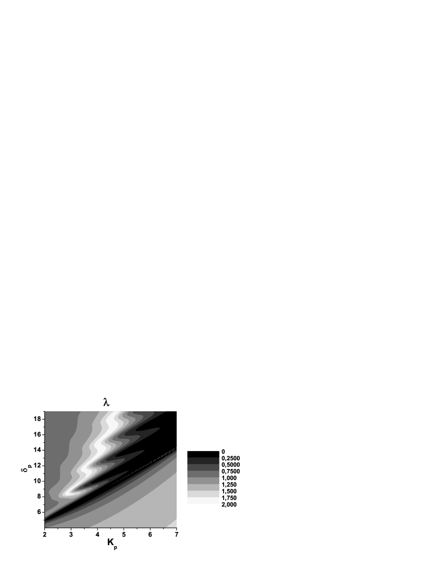
Figure 4: Topological graph of principal squeeze variance $\lambda$ in mode ($s_{F},i_{F}$) as it depends on linear coupling constant $K_{p}$ and linear phase mismatch $\delta_{p}$ between the pump fields; $L=2$, $A_{p_{F}}=10$, $\delta_{F}=\delta_{B}=5$, and values of the other parameters are the same as in Fig. 2.

The possibility to compensate for a nonlinear phase-mismatch using linear coupling between modes has been discussed in PoDong2004 from the point of view of efficiency of energy conversion.

Nonlinear phase mismatch $\delta_{nl}$ can be also compensated using nonzero incident amplitudes of the backward-propagating pump mode. We have found the optimum value of the phase difference between the forward-propagating pump amplitude and backward-propagating pump amplitude to be $3\pi/2$ [$\pi/2$] for mode ($s_{F},i_{F}$) [($s_{B},i_{B}$)] with respect to squeezed-light generation.

Now we assume linear scattering of pump, signal, and idler fields ($K_{p}\neq 0$, $K_{s}\neq 0$, $K_{i}\neq 0$). The analysis of squeezed-light generation is difficult under these conditions because every linear coupling constant introduces some phase changes along the waveguide that modify the nonlinear interaction. In general, squeezing can be observed in modes ($s_{F},i_{F}$), ($s_{B},i_{B}$), and ($s_{F},i_{B}$) under suitably chosen values of parameters. The occurrence of squeezing in mode ($s_{F},i_{B}$) originates in linear scattering of the down-converted fields.

Nonzero values of $K_{s}$ and $K_{i}$ support squeezed-light generation in mode ($s_{B},i_{B}$), because they transfer energy from modes $s_{F}$ and $i_{F}$ into modes $s_{B}$ and $i_{B}$ and so the nonlinear interaction among the backward-propagating fields can have also a strong stimulated part. A nonzero value of $K_{i}$ is also indispensable for observing squeezing in mode ($s_{F},i_{B}$), because “an already generated squeezed light in the nonlinear interaction among the forward-propagating fields has to be transferred into mode $i_{B}$”.

Being in non-oscillating regime of behavior of amplitude mean-values ($\delta_{p}<2|K_{p}|$, $\delta_{s}<2|K_{s}|$, $\delta_{i}<2|K_{i}|$) lower values of $\lambda$ can be reached in mode ($s_{B},i_{B}$) in comparison with those reached in mode ($s_{F},i_{F}$) probably because modes $s_{B}$ and $i_{B}$ begin the nonlinear interaction in the vacuum states and so phases of their amplitudes can be suitably set in the interaction. In general, the regime with the oscillating behavior of amplitude mean-values ($\delta_{p}>2|K_{p}|$, $\delta_{s}>2|K_{s}|$, $\delta_{i}>2|K_{i}|$) is better for squeezed-light generation and low values of principal squeeze variances $\lambda$ can be reached in this regime. Squeezing can be observed under a wide range of values of parameters in non-oscillating regime in modes ($s_{F},i_{F}$), ($s_{B},i_{B}$), and ($s_{F},i_{B}$). We note, that greater values of, e.g., $\delta_{i}$ effectively decrease the value of $K_{i}$ which acts against squeezed-light generation in mode ($s_{F},i_{B}$). A difference in the ability to generate squeezed-light in oscillating and non-oscillating regimes is clearly visible in Fig. 5, where principal squeeze variance $\lambda$ of mode ($s_{F},i_{B}$) is plotted as a function of linear phase mismatches $\delta_{s}$ and $\delta_{i}$.

Figure 5: Principal squeeze variance $\lambda$ of mode ($s_{F},i_{F}$) as a function of linear phase mismatches $\delta_{s}$ and $\delta_{i}$ between the signal and idler fields, respectively; $L=2$, $K_{p}=5$, $K_{s}=K_{i}=5$, $A_{p_{F}}=10$, and values of the other parameters are the same as in Fig. 2.

As can be shown directly by a suitable substitution into Eqs. (5) and (10), their solutions depend only on the overall phase $\psi=-\arg(K_{p})+\arg(K_{s})+\arg(K_{i})$ of the linear coupling constants. In our investigations, principal squeeze variances $\lambda$ in modes ($s_{F},i_{F}$) and ($s_{B},i_{B}$) had minimum values for $\psi=\pi/2$ and $\lambda$ in mode ($s_{F},i_{B}$) reached its lowest value for $\psi=3\pi/2$. Also the dependence of principal squeeze variances $\lambda$ on phases of the incident forward-propagating signal and idler fields have not been observed.

At the end of the discussion of squeezing we mention the case in which, e.g., the incident forward-propagating signal field is stronger than the incident forward-propagating pump field. We then have squeezing also in compound modes that combine one pump field with one down-converted field under suitably chosen values of parameters. In general, values of principal squeeze variances $\lambda$ are lower in these compound modes that contain a down-converted field with great values of amplitudes inside the structure.

IV Photon-number statistics

When a field is detected by a classical detector statistical properties of the incident field are suitably described by normally-ordered moments of integrated intensity $\hat{W}$ ($\hat{W}=\hat{A}^{\dagger}\hat{A}$):

$$\langle W^{k}\rangle_{\cal N}=\langle\hat{A}^{\dagger k}\hat{A}^{k}\rangle,\hskip 28.45274ptk=2,3,\ldots,$$ (22)

where $\hat{A}$ denotes an electric-field-amplitude operator of the incident optical field.

Type of a statistical distribution of photoelectrons emitted inside the detector can be determined using Fano factor $F_{n}$. Fano factor $F_{n}$ can be expressed in terms of normally-ordered moments of integrated intensity $\hat{W}$ as follows:

$$F_{n}=\frac{\langle(\Delta n)^{2}\rangle}{\langle n\rangle}=1+\frac{\langle(\Delta W)^{2}\rangle_{\cal N}}{\langle W\rangle_{\cal N}}.$$ (23)

Symbol $n$ denotes the number of photoelectrons, $\Delta n=n-\langle n\rangle$, and $\Delta W=W-\langle W\rangle_{\cal N}$. Intensity operator $\hat{W}_{ij}$ of a compound mode ($i,j$) is then determined along the relation $\hat{W}_{ij}=\hat{W}_{i}+\hat{W}_{j}$, where $\hat{W}_{i}$ ($\hat{W}_{j}$) stands for the intensity operator of mode $i$ ($j$). Classical fields obey the inequality $F_{n}\geq 1$. On the other hand values of Fano factor $F_{n}$ smaller than one can be reached considering nonclassical fields (sub-Poissonian light). The condition $F_{n}\leq 1$ means that fluctuations in the number of photoelectrons are suppressed below the classical limit that is given by the Poissonian photon-number statistics of a laser radiation.

Assuming that the outgoing fields can be described in the framework of the generalized superposition of signal and noise, moments of integrated intensity $\hat{W}$ can be written as:

$$\langle W_{j}\rangle_{\cal N} = B_{j}+|\xi_{j}|^{2},$$

$$\langle(\Delta W_{j})^{2}\rangle_{\cal N} = B_{j}^{2}+|C_{j}|^{2}+2B_{j}|\xi_{j}|^{2}+\left(C_{j}\xi_{j}^{*2}+{\rm c.c.}\right),$$

$$\langle\Delta W_{j}\Delta W_{k}\rangle_{\cal N} = |D_{jk}|^{2}+|\bar{D}_{jk}|^{2}$$ (24)

$$\mbox{}+\left(D_{jk}\xi_{j}^{*}\xi_{k}^{*}-\bar{D}_{jk}\xi_{j}\xi_{k}^{*}+{\rm c.c.}\right).$$

Coefficients $B_{j}$, $C_{j}$, $D_{jk}$, and $\bar{D}_{jk}$ are given in Eqs. (19). Symbol $\xi_{j}$ in Eqs. (24) denotes a coherent amplitude of the $j$th outgoing field. We note that photon-number distribution as well as moments of integrated intensity can be determined in general using an expansion into Laguerre polynomials (see, e.g., Perina1991 ; Perinova1981 ).

Nonclassical character of photon-number statistics occurs mostly at single-photon level. For this reason, we assume a regime in which the waveguide is pumped by a strong forward-propagating pump field and classical strong amplitude mean-values $A_{s_{F}}$, $A_{i_{F}}$, $A_{s_{B}}$, and $A_{i_{B}}$ are zero. Operator amplitudes $\hat{A}$ of the signal and idler fields are then given just by their linear operator amplitude corrections $\delta\hat{A}$. We also assume that the incident fields described only by linear operator amplitude corrections are coherent and denote their amplitudes by $\xi$.

Assuming $K_{s}L$, $K_{i}L$, $K_{p}L$, $K_{F}AL$ ($A$ being a typical field amplitude), and $K_{B}AL$ being small, expressions for first and second moments of integrated intensity $\hat{W}$ can be found as it was done in PerinaJr2004 . This approximation gives the same expressions as those published in Eqs. (30) and (31) in PerinaJr2004 for the case $K_{p}=0$; i.e. no conclusion about the influence of $K_{p}$ can be deduced.

We first consider a phase-matched nonlinear waveguide with no photonic band-gap structure ($K_{s}=K_{i}=K_{p}=0$). Sub-Poissonian light in mode ($s_{F},i_{F}$) can occur for a sufficiently strong pumping. However, as Fig. 6 shows, if the value of pump amplitude $A_{p_{F}}$ is too great, sub-Poissonian character of the generated light is lost.

Figure 6: Fano factor $F_{n}$ of mode ($s_{F},i_{F}$) as a function of forward-propagating pump amplitude $A_{p_{F}}$; input linear operator amplitude corrections $\delta\hat{A}$ are assumed to be in coherent states with amplitudes $\xi$, amplitudes $\xi$ are expressed in units of 10 Vm^-1 and so mean values of intensities are directly equal to mean photon numbers; $L=2$, $K_{F}=K_{B}=5\times 10^{-2}$, $K_{p}=K_{s}=K_{i}=0$, $\delta_{p}=\delta_{s}=\delta_{i}=0$, $\delta_{F}=\delta_{B}=0$, $A_{p_{F}}=10$, $A_{s_{F}}=A_{i_{F}}=0$, $A_{p_{B}}=A_{s_{B}}=A_{i_{B}}=0$; $\xi_{s_{F}}=-10$, $\xi_{i_{F}}=10$ $\xi_{p_{F}}=\xi_{s_{B}}=\xi_{i_{B}}=\xi_{p_{B}}=0$.

Suitable values of pump amplitude $A_{p_{F}}$ for sub-Poissonian-light generation depend on length $L$ of the waveguide. The longer the waveguide, the smaller the suitable values of pump amplitude $A_{p_{F}}$. A photonic band-gap structure with $K_{p}\neq 0$ (also $K_{s}=K_{i}=0$ is assumed) inside the waveguide in this case leads to a redistribution of energy in the pump modes in the way that enables again sub-Poissonian-light generation in mode ($s_{F},i_{F}$). For a given value of length $L$ and a given sufficiently great value of $A_{p_{F}}$ there is an optimum value of $K_{p}$ for which the value of Fano factor $F_{n}$ reaches a minimum value that is obtained also in the waveguide without a photonic band-gap structure ($F_{n}\approx 0.3$, see Fig. 7). If the value of pump amplitude $A_{p_{F}}$ is small, the greater the $K_{p}$ the greater the Fano factor $F_{n}$; i.e. a photonic band-gap structure does not support sub-Poissonian-light generation in this case.

Figure 7: Fano factor $F_{n}$ of mode ($s_{F},i_{F}$) as a function linear coupling constant $K_{p}$ between the pump fields; $A_{p_{F}}=10$ and values of the other parameters are the same as in Fig. 6.

Nonzero values of linear phase mismatch $\delta_{p}$ in this otherwise phase-matched interaction result in greater values of Fano factor $F_{n}$.

In order to obtain sub-Poissonian light in mode ($s_{F},i_{F}$), the nonlinear interaction has to be stimulated, i.e. the incident small amplitudes $\xi_{s_{F}}$ and $\xi_{i_{F}}$ have to be nonzero. Moreover, values of amplitudes $\xi_{s_{F}}$ and $\xi_{i_{F}}$ have to be nearly the same and their phases have to fulfill the condition $\arg(\xi_{s_{F}})+\arg(\xi_{i_{F}})\approx\pi$. Under these conditions Fano factor $F_{n}$ of mode ($s_{F},i_{F}$) decreases with increasing values of amplitudes $\xi_{s_{F}}$ and $\xi_{i_{F}}$. For a certain value of these amplitudes a minimum value of Fano factor $F_{n}$ is reached. In our case this occurs for approximately 100 incident photons in both forward-propagating signal and idler fields, as is shown in Fig. 8.

Figure 8: Fano factor $F_{n}$ of mode ($s_{F},i_{F}$) as a function of amplitude $\xi$: $\xi_{s_{F}}=-\xi$, $\xi_{i_{F}}=\xi$: $K_{p}=1.4$, $A_{p_{F}}=10$, and values of the other parameters are the same as in Fig. 6.

If the nonlinear interaction is not phase-matched ($\delta_{nl}=\delta_{F}=\delta_{B}\neq 0$) in the waveguide with no photonic band-gap structure ($K_{s}=K_{i}=K_{p}=0$) sub-Poissonian light in mode ($s_{F},i_{F}$) can still be obtained but greater values of Fano factor $F_{n}$ occur. Even values of Fano factor $F_{n}$ can monotonically increase as the value of pump amplitude $A_{p_{F}}$ increases in some cases. Then values of parameters of the photonic band-gap structure ($K_{p}\neq 0$, $\delta_{p}\neq 0$, $K_{s}=K_{i}=0$) can be set in such a way that the original low values of Fano factor $F_{n}$ are restored. If we consider $\delta_{nl}=5$ mm^-1 under the conditions specified in caption to Fig. 6, the lowest value of Fano factor $F_{n}$ is approximately 0.8. A suitable choice of values of $K_{p}$ and $\delta_{p}$ provides the original value of Fano factor $F_{n}$ being roughly 0.3, as is documented in Fig.9. According to our investigations, the region in $(K_{p},\delta_{p})$ space for which the influence of nonlinear phase mismatch $\delta_{nl}$ is compensated lies around $\delta_{p}\approx 2|K_{p}|$ and also greater values of $K_{p}$ are needed. As is seen from Fig. 9, the region where $\delta_{p}$ is greater than $2|K_{p}|$ is not suitable for the generation of sub-Poissonian light.

Figure 9: Topological graph of Fano factor $F_{n}$ of mode ($s_{F},i_{F}$) in dependence on linear coupling constant $K_{p}$ and linear phase mismatch $\delta_{p}$ between the pump fields; only values of $F_{n}$ lower than 1 are plotted; $L=1$, $\delta_{F}=\delta_{B}=5$, $A_{p_{F}}=10$, and values of the other parameters are the same as in Fig. 6.

A suitable choice of the incident phase $\varphi_{p_{F}}$ of the forward-propagating pump mode [$\varphi_{p_{F}}=\arg(A_{p_{F}})$] can be used as a final step to reach the lowest possible value of Fano factor $F_{n}$ that is allowed by a given set of values of waveguide parameters. We have observed a strong dependence of values of Fano factor $F_{n}$ on the value of phase $\varphi_{p_{F}}$.

Low values of Fano factor $F_{n}$ are usually reached when also integrated intensity $W$ of a given mode has low values.

We now consider the influence of photonic band-gap structure in its full complexity, i.e. also the signal and idler fields are linearly scattered ($K_{s}\neq 0$, $K_{i}\neq 0$). Under phase-matched conditions increasing values of $K_{s}$ and $K_{i}$ destroy sub-Poissonian photon-number statistics in mode ($s_{F},i_{F}$) (see Fig. 10).

Figure 10: Fano factor $F_{n}$ of mode ($s_{F},i_{F}$) in dependence on linear coupling constants $K_{s}$ and $K_{i}$ between the signal and idler fields; $K_{p}=1.4$, $A_{p_{F}}=10$, and values of the other parameters are the same as in Fig. 6.

On the other hand, they support sub-Poissonian-light generation in modes ($s_{B},i_{B}$) and ($s_{F},i_{B}$). Mode ($s_{F},i_{B}$) can have values of Fano factor $F_{n}$ less than one only for small values of $K_{s}$ and also a nonzero value of $K_{i}$ is required. In general, oscillating regime of behavior of field amplitudes ($\delta_{s}>2|K_{s}|$, $\delta_{i}>2|K_{i}|$, $\delta_{p}>2|K_{p}|$) is more convenient for sub-Poisonian-light generation.

Values of Fano factors $F_{n}$ in general depend only on the phase $\psi$ [$\psi=-\arg(K_{p})+\arg(K_{s})+\arg(K_{i})$] that combines phases of all linear coupling constants. The lowest value of Fano factor $F_{n}$ in mode ($s_{B},i_{B}$) is reached for $\psi=\pi/2$; $\psi=3\pi/2$ has been found to be optimum for mode ($s_{F},i_{B}$).

We note that a qualitative similarity can be found in the behavior of photon-number statistics between the investigated waveguide and that one composed of two separated nonlinear parts with co-propagating fields Mista1999 .

V Increase of intensity signal-to-noise ratio

The nonlinear waveguide can also be used for improving signal-to-noise ratio of an incident field. This effect can be explained claiming that the signal part and the noisy part of the incident field have different amplification coefficients in the nonlinear process. An average amplification coefficient of a field in a nonlinear process depends on a statistical distribution of incident-field phases; there exists one phase for which the amplification is maximum. If the central phase of the incident field (corresponding to a coherent signal amplitude) has the strongest amplification then the noisy part (with a blurred phase distribution) is less amplified on average and signal-to-noise ratio increases.

Similarly as for sub-Poissonian-light generation, the best conditions for the reduction of noise-to-signal ratio can be found in a phase-matched waveguide without a photonic band-gap structure. If nonlinear phase-matching cannot be reached, a suitable photonic band-gap structure inside the waveguide compensates for nonlinear phase-mismatch and gives similar conditions for the reduction of noise-to-signal ratio as those found in the perfectly phase-matched waveguide. For a given value of nonlinear phase mismatch $\delta_{nl}$ ($\delta_{nl}=\delta_{F}=\delta_{B}$), there are regions in space $(K_{p},\delta_{p})$ where the optimum conditions for the reduction of noise-to-signal ratio are found. These regions lie around the line $\delta_{p}=2|K_{p}|$ and also values of $K_{p}$ have to be greater. Second reduced moment of integrated intensity $R_{W}$ [$R_{W}=\langle W^{2}\rangle_{\cal N}/\langle W\rangle_{\cal N}^{2}$] for mode $s_{F}$ having incident $R_{W}=1.75$ (100 incident signal photons, 100 incident noisy photons) is plotted in Fig. 11 assuming $\delta_{nl}=5$ mm^-1. Regions suitable for the reduction of noise-to-signal ratio are visible in Fig. 11; the lowest achieved value of $R_{W}$ is 1.36.

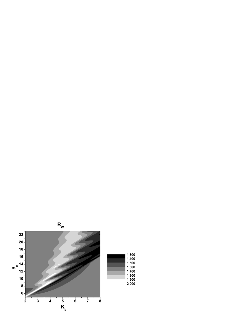
Figure 11: Topological graph of second reduced moment $R_{W}$ of integrated intensity in mode $s_{F}$ as a function of linear coupling constant $K_{p}$ and linear phase mismatch $\delta_{p}$ between the pump fields; an incident value of $R_{W}$ equals 1.75; $A_{p_{F}}=10$, $\delta_{F}=\delta_{B}=5$, $\xi_{s_{F}}=\xi_{i_{F}}=10$, $n_{{\rm ch},s_{F}}=100$, $n_{{\rm ch},i_{F}}=0$, and values of the other parameters are the same as in Fig. 6.

Capability to reduce noise-to-signal ratio increases with the increasing forward-propagating pump amplitude $A_{p_{F}}$ (see Fig. 12). This monotonous behavior clearly shows that the nonlinear interaction is responsible for this effect. The strength of the effect also depends on the amount of incident noise. As demonstrated in Fig. 12 for mode $s_{F}$, an optimum value of the number of incident noisy photons exists for which the reduction of noise-to-signal ratio is the best.

Figure 12: Relative second reduced moment $T_{W}$ of integrated intensity in mode $s_{F}$ as a function of forward-propagating pump amplitude $A_{p_{F}}$ and number $n_{{\rm ch},s_{F}}$ of incident chaotic photons in this mode; $T_{W}=R_{W}^{\rm out}/R_{W}^{\rm in}$ where $R_{W}^{\rm in}$ ($R_{W}^{\rm out}$) characterizes the incident (outgoing) field; $K_{p}=8$, $\delta_{p}=20$, $\delta_{F}=\delta_{B}=5$, $\xi_{s_{F}}=\xi_{i_{F}}=10$, $n_{{\rm ch},i_{F}}=0$, and values of the other parameters are the same as in Fig. 6.

VI Conclusions

A planar nonlinear photonic band-gap waveguide with optical parametric process has been analyzed from the point of view of generation of squeezed light and light with sub-Poissonian photon-number statistics. It has been shown that squeezed light as well as sub-Poissonian light can be generated in compound modes composed of one signal and one idler field; both forward- and backward-propagating fields can be successfully combined. The waveguide with a photonic band-gap structure cannot provide better values of principal squeeze variance and Fano factor in comparison with the waveguide with no photonic band-gap structure and having the nonlinear interaction phase-matched. However, if the nonlinear interaction in a waveguide cannot be phase-matched for some reason, inclusion of a photonic band-gap structure such as to compensate for phase mismatch leads to values of principal squeeze variances and Fano factors that are found assuming perfect phase-matching. This property makes nonlinear photonic band-gap waveguides promising as sources of light with nonclassical properties. Moreover, if a noisy light is incident on the waveguide its signal-to-noise ratio can be improved as the light propagates in the waveguide.

- (1) M. Bertolotti, C.M. Bowden, and C. Sibilia, Nanoscale Linear and Nonlinear Optics, AIP Vol. 560 (AIP, Melville, 2001).
- (2) J.D. Joannopoulos, R.D. Meade, and J.N. Winn, Photonic Crystals: Molding the Flow of Light (Princeton University Press, Princeton, 1995).
- (3) M. Scalora, M.J. Bloemer, A.S. Manka, J.P. Dowling, C.M. Bowden, R. Viswanathan, and J.W. Haus, Phys. Rev. A 56, 3166 (1997).
- (4) Y. Dumeige, P. Vidakovic, S. Sauvage, I. Sagnes, J.A. Levenson, C. Sibilia, M. Centini, G. D’Aguanno, and M. Scalora, Appl. Phys. Lett. 78, 3021 (2001).
- (5) K. Sakoda, J. Opt. Soc. Am. B 19, 2060 (2002).
- (6) D. Tricca, C. Sibilia, S. Severini, M. Bertolotti, M. Scalora, C.M. Bowden, and K. Sakoda, J. Opt. Soc. Am. B 21, 671 (2004).
- (7) J. Peřina Jr., C. Sibilia, D. Tricca, and M. Bertolotti, Phys. Rev. A 70, 043816 (2004); quant-ph/0405051.
- (8) J. Peřina Jr. and J. Peřina, Progress in Optics 41, Ed. E. Wolf, (Elsevier Science, Amsterdam, 2000), p. 362.
- (9) P. Yeh, Optical Waves in Layered Media (Wiley, New York, 1988).
- (10) D. Pezzetta, C. Sibilia, M. Bertolotti, J.W. Haus, M. Scalora, M.J. Bloemer, and C.M. Bowden, J. Opt. Soc. Am. B 18, 1326 (2001).
- (11) W.H. Press, S.A. Teukolsky, W.T. Vetterling, and B.P. Flannery, Numerical Recipes (Cambridge University Press, Cambridge, 1996).
- (12) A. Luis and J. Peřina, Quantum Semiclass. Opt. 8, 39 (1996).
- (13) J. Peřina, Quantum Statistics of Linear and Nonlinear Optical Phenomena (Kluwer, Dordrecht, 1991).
- (14) A. Lukš, V. Peřinová, and J. Peřina, Opt. Commun. 67, 149 (1988).
- (15) J. Herec, Acta Phys. Slovaka 49, 731 (1999).
- (16) L. Mišta Jr., Acta Phys. Slovaka 49, 737 (1999).
- (17) P. Dong and A.G. Kirk, Phys. Rev. Lett. 93, 133901 (2004).
- (18) V. Peřinová, Optica Acta 28, 747 (1981); V. Peřinová and J. Peřina, Optica Acta 28, 769 (1981).