Exploring a New Post-Selection Condition for Efficient Linear Optics Quantum Computation

Abstract

Recently, it was shown that fundamental gates for theoretically efficient quantum information processing can be realized by using single photon sources, linear optics and quantum counters. One of these fundamental gates is the NS-gate, that is, the one-mode non-linear sign shift. In this work, firstly, we prove by a new rigorous proof that the upper bound of success probability of NS-gates with only one helper photon and an undefined number of ancillary modes is bounded by $0.25$. Secondly, we explore the upper bound of success probability of NS-gate with a new post-selection measurement. The idea behind this new post-selection measurement is to condition the success of NS-gate transformation to the observation of only one helper photon in whichever of the output modes.

1 Introduction to Conditional Operations

Linear optical passive (LOP) transformations are defined as the class of linear optical transformations that act on the system of $N$ optical modes leaving unchanged the total number of photons in the process. With every LOP one can associate three mathematical objects: the $N\times N$ unitary matrix $\underline{U}$ describing the transformation on the field operators of the $N$ optical modes, the unitary operator $U$ acting by similarity on the field operators, and the unitary infinite matrix $\overline{U}$ representing $U$ on the Fock space of the optical modes.

In the context of quantum computing and quantum information processing, several conditional schemes have been proposed [1, 2, 3, 4, 5, 6, 7] to perform a wider class of transformations. It is still an open problem the complete classification of this wider class [8, 9, 10]. However, the general scheme has a conceptually simple two step structure. At first, one couples the $N$ mode system with $k$ ancillary modes and let the two transform under a global LOP, corresponding to a unitary evolution of the bipartite system. Then one performs a measurement on the ancillae and selects the output state of the system only when a predefined result is obtained: thisi is called post selection. This procedure in general will transform the state of the system as a completely positive map (CP).

These schemes are referred to as conditional because the implemented transformations are conditioned by a predefined measurement outcome. Moreover, these schemes are referred to as non-deterministic because there is some probability that a different outcome is obtained (i.e. the schemes implement a transformation that is not the desired one).

We start introducing some notation: let us denote with $\mathscr{H}_{S}$ the Hilbert space on which the logical system is encoded. Indeed, logical states can be encoded in a subspace of the $N$ mode Fock space or more in general in the direct sum of several such subspaces. So we can write: $\mathscr{H}_{S}=\bigoplus_{n}\mathscr{H}_{n_{S}}^{(N)}$, where we denote by $\mathscr{H}_{n_{S}}^{(N)}$ the space spanned by the states of $n_{S}$ photons distributed on the $N$ modes.

Let $\rho$ be the input state of the system, i.e. a density matrix on $\mathscr{H}_{S}$, and $\sigma$ the ancilla input state, and we assume that $\sigma$ is a pure Fock state with exactly $n_{A}$ photons, i.e. a rank $1$ projector on the Hilbert space: $\mathscr{H}_{A}=\mathscr{H}_{n_{A}}^{(k)}$. If the ancilla and the system do not interact during their preparation, the global input state is not an entangled one, so that we can write it as: $\rho\otimes\sigma$.

The effect on the system of the global LOP can be described by the expression $U(\rho\otimes\sigma)U^{{\dagger}}$, which corresponds a mixed output with respect to the system S: $\rho^{{}^{\prime}}=\textrm{tr}_{A}(U(\rho\otimes\sigma)U^{{\dagger}})$. It is well known that this transformation can be described by a trace preserving CP map $\tau$ for which one can always find a operator sum representation:

$$\rho^{{}^{\prime}}=\tau(\rho)=\sum_{\mu}M_{\mu}\rho M_{\mu}^{{\dagger}}$$

$$\sum_{\mu}M_{\mu}^{{\dagger}}M_{\mu}=\mathbb{I}$$ (1)

After a suitable relabeling of $\mathscr{H}_{S}$ and $\mathscr{H}_{A}$, denoting with $\{|\alpha\rangle_{S}\}$ and $\{|\nu\rangle_{A}\}$ their respective basis, $\rho$ and $\sigma$ can be decomposed as:

$$\left\{\begin{array}[]{ccc}\rho&=&\sum_{\alpha,\beta}\rho_{\alpha\beta}|\alpha\rangle_{S}\langle\beta|\\ \sigma&=&|\nu\rangle_{A}\langle\nu|\end{array}\right.$$ (2)

Using these expressions we can explicitly evaluate the partial trace obtaining the output density matrix of the system S,

$$\rho^{{}^{\prime}}_{\gamma\delta} = \sum_{\mu}\sum_{\alpha,\beta}(\langle\mu^{{}^{\prime}}|\otimes\langle\gamma^{{}^{\prime}}|U|\alpha\rangle\otimes|\nu\rangle)$$ (3)

$$\rho_{\alpha\beta}(\langle\nu|\otimes\langle\beta|U^{{\dagger}}|\delta^{{}^{\prime}}\rangle\otimes|\mu^{{}^{\prime}}\rangle)$$

and so the matrix elements of $M_{\mu}$ are given by:

$$(M_{\mu}^{(\nu)})_{\gamma}^{\alpha}=\langle\mu^{{}^{\prime}}|\otimes\langle\gamma^{{}^{\prime}}|U|\alpha\rangle\otimes|\nu\rangle$$ (4)

where index $\nu$ is fixed by the ancilla input, index $\mu$ is related to the post-selection condition, and $\gamma,\alpha$ run through matrix elements. It is easy to verify that unitarity of $U$ guarantees condition 1.

We consider the case in which this is described by a Projective Valued Measure (PVM) associated to the basis $\{|\mu^{{}^{\prime}}\rangle\}$, namely by rank $r$ projectors:

$$P_{\mu}=\mathbb{I}_{S}\otimes\sum_{\mu}s_{\mu}|\mu^{{}^{\prime}}\rangle\langle\mu^{{}^{\prime}}|$$ (5)

with exactly $r$ terms in which $s_{\mu}=1$, and all the others with $s_{\mu}=0$.

Now, the conditional (unnormalized) output state is:

$$\bar{\rho}=\textrm{tr}_{A}(P_{\mu}U(\rho\otimes\sigma)U^{{\dagger}}P_{\mu})=M_{\mu}\rho M_{\mu}^{{\dagger}}$$ (6)

with probability

$$p_{\mu}=\textrm{tr}_{S}\textrm{tr}_{A}(U(\rho\otimes\sigma)U^{{\dagger}}P_{\mu})=\textrm{tr}_{\bar{S}}(M_{\mu}\rho M_{\mu}^{{\dagger}})$$ (7)

Of course the normalized output state is given by $\bar{\rho}_{\textrm{\footnotesize{norm}}}=\frac{\bar{\rho}}{p_{\mu}}$.

2 Non-Linear Sign-Shift Gate

2.1 Gate Operation

Now, we are interested in analyzing the implementation of the one-mode non-linear sign-shift (NS) on the 2-photons Fock state:

$$|\psi\rangle=\alpha|0\rangle+\beta|1\rangle+\gamma|2\rangle\longrightarrow|\psi^{{}^{\prime}}\rangle=\alpha|0\rangle+\beta|1\rangle-\gamma|2\rangle$$ (8)

as a conditional operation. This transformation is not realizable as a one-mode LOP (hence the name non-linear). So we consider the conditional scheme proposed by KLM uses two ancillary modes prepared in the state, $\sigma=|10\rangle_{A}\langle 10|$, and the post-selection condition described by the rank-1 projector, $P_{10}=\mathbb{I}_{S}\otimes|10\rangle_{A}\langle 10|$. The corresponding non-unitary operator is represented by the matrix:

$$(M_{10}^{(10)})_{n^{{}^{\prime}}}^{n}={}_{A}\langle 10|\otimes{}_{S}\langle n^{{}^{\prime}}|U|n\rangle_{S}\otimes|10\rangle_{A}$$ (9)

where $|n\rangle_{S}$ is the $n$-photon Fock state. The conservation of the total number of photons implies that $M_{10}^{(10)}$ should be a diagonal matrix, since non-vanishing terms are those with $n=n^{{}^{\prime}}$, and by a straightforward calculation one finds:

$$(M_{10}^{(10)})_{0}^{0}= \overline{U}_{010}^{010} =\underline{U}_{22}$$

$$(M_{10}^{(10)})_{1}^{1}= \overline{U}_{110}^{110} =\underline{U}_{11}\underline{U}_{22}+\underline{U}_{12}\underline{U}_{21}$$

$$(M_{10}^{(10)})_{2}^{2}= \overline{U}_{210}^{210} =\underline{U}_{11}(\underline{U}_{11}\underline{U}_{22}+2\underline{U}_{12}\underline{U}_{21})$$ (10)

For the operation to implement the desired sign-shift, one must ask that $\underline{U}$ is such that:

$$(M_{10}^{(10)})_{0}^{0}=(M_{10}^{(10)})_{1}^{1}=-(M_{10}^{(10)})_{2}^{2}$$ (11)

which means that,

$$\underline{U}_{11} = 1-\sqrt{2}$$

$$\underline{U}_{22} = \frac{\underline{U}_{12}\underline{U}_{21}}{1-\underline{U}_{11}}$$ (12)

The success probability is obtained simply applying (7):

$$p_{10}=|(M_{10}^{(10)})_{0}^{0}|^{2}=|\underline{U}_{22}|^{2}$$ (13)

and it is maximum when $\underline{U}_{12}=\underline{U}_{21}=2^{-\frac{1}{4}}$, which gives $p_{10}=\frac{1}{4}$.

Two possible circuits implementing this operation are shown in [1, 3].

2.2 General Bound with One Ancillary Photon

In this section we show that the maximum value for $p_{\mu}$ when only one ancillary photon is present at the input cannot be increased by adding any arbitrary number of ancillary modes prepared in the vacuum state.

Let us suppose that we have a $k$-modes initial ancillary state, $\sigma_{i}=|\mathbf{i}\rangle_{A}\langle\mathbf{i}|$, where $|\mathbf{i}\rangle_{A}$ is the state with one photon injected in the $i$-th mode, and a post-selection condition, $P_{j}=\mathbb{I}_{S}\otimes|\mathbf{j}\rangle_{A}\langle\mathbf{j}|$.

It should be clear that whichever input state $\sigma_{l}$ is related to $\sigma_{i}$ by a simple permutation, namely a swapping of two modes that can be done deterministically, and the same holds for any post-selection condition $P_{l}$. From a mathematical viewpoint, it simply consists in the exchange of two rows, or two columns of $\underline{U}$.

We first impose the functioning conditions, and then study the probability under the request that the matrix $\underline{U}$ should be unitary in order to be implementable by a LOP circuit. It is simple to show that the $(k+1)\times(k+1)$ matrix $\underline{U}$ must satisfy the same conditions as in (2.1), but with column index $2$ replaced by $i$ and row index $2$ replaced by $j$. Thus one can write:

$$\left(\begin{array}[]{cccc}1-\sqrt{2}&\ldots&\underline{U}_{1,i}&\ldots\\ \vdots&{}\hfil&\vdots&{}\hfil\\ \underline{U}_{j,1}&\ldots&\frac{\underline{U}_{1,i}\underline{U}_{j,1}}{\sqrt{2}}&\ldots\\ \vdots&{}\hfil&\vdots&\ddots\end{array}\right)$$ (14)

Now, the probability is equal to $\frac{\underline{U}_{1,i}\underline{U}_{j,1}}{\sqrt{2}}$, and it has to be maximized under the condition that $\underline{U}$ be unitary. We note that it suffices to impose that the first and the $j$-th row are mutually orthogonal, and that they are normalizable together with the first and the $i$-th column, namely:

$$\sum_{l}\underline{U}_{1,l}=1=\sum_{l}\underline{U}_{j,l}\quad\sum_{l}\underline{U}_{l,1}=1=\sum_{l}\underline{U}_{l,i}\quad$$ (15)

When one has two orthonormal rows, the whole matrix can be constructed simply by completing the set of orthonormal vectors arbitrarily, since all other matrix elements do not enter into the functioning conditions. Normalizability is expressed by:

$$\left\{\begin{array}[]{ccc}\textrm{row}\quad 1&\rightarrow&|U_{1,i}|^{2}\leq 2(\sqrt{2}-1)\\ \textrm{row}\quad j&\rightarrow&|U_{j,1}|^{2}\leq\left(1+\frac{|U_{1,i}|^{2}}{2}\right)^{-1}\\ \textrm{column}\quad 1&\rightarrow&|U_{j,1}|^{2}\leq 2(\sqrt{2}-1)\\ \textrm{column}\quad i&\rightarrow&|U_{1,i}|^{2}\leq\left(1+\frac{|U_{j,1}|^{2}}{2}\right)^{-1}\end{array}\right.$$ (17)

and this furnishes a limitation for the region in which $|U_{1,i}|$ and $|U_{j,1}|$ can take values (see fig.1).

To impose orthogonality of two rows of arbitrary length, we define the two $(k-1)$-components complex vectors $\vec{v}_{(1)},\vec{v}_{(j)}$:

$$\vec{v}_{(1)}^{\top} = (U_{1,2},\ldots,U_{1,i-1},U_{1,i+1},\ldots,U_{1,k+1})$$ (18)

$$\vec{v}_{(j)}^{\top} = (U_{j,2},\ldots,U_{j,i-1},U_{j,i+1},\ldots,U_{j,k+1})$$ (19)

such that normalization of the rows is completed

$$\left\{\begin{array}[]{c}|\vec{v}_{(1)}|^{2}=2(\sqrt{2}-1)-|U_{1,i}|^{2}\\ |\vec{v}_{(j)}|^{2}=1-|U_{j,1}|^{2}\left(1+\frac{|U_{1,i}|^{2}}{2}\right)\end{array}\right.$$ (20)

and orthogonality is satisfied

$$\vec{v}_{(1)}^{{\dagger}}\cdot\vec{v}_{(j)}=-U_{j,1}\left(1-\sqrt{2}+\frac{|U_{1,i}|^{2}}{\sqrt{2}}\right)$$ (21)

Here $\vec{v}_{(1)}^{{\dagger}}$ denotes the hermitian conjugate of $\vec{v}_{(1)}$, namely the row whose elements are the complex conjugate of those of $\vec{v}_{(1)}$. Now, we notice that in a complex vector space, making use of the Schwartz inequality, the scalar product can be written as:

$$\vec{v}_{(1)}^{{\dagger}}\cdot\vec{v}_{(j)}=e^{i\phi}|\vec{v}_{(1)}||\vec{v}_{(j)}|\cos\alpha_{1j}$$ (22)

and upon substitution $U_{j,1}=e^{i\phi_{j1}}|U_{j,1}|$, we can separate eq. (21) in phase and modulus:

$$\left\{\begin{array}[]{c}\phi=\phi_{j1}\pm\pi\\ |\vec{v}_{(1)}^{{\dagger}}\cdot\vec{v}_{(j)}|=|U_{j,1}|\left|\left(1-\sqrt{2}+\frac{|U_{1,i}|^{2}}{\sqrt{2}}\right)\right|\end{array}\right.$$ (23)

After some substitutions, one gets:

$$|\cos\alpha_{1j}|=\frac{|U_{j,1}||(1-\sqrt{2})+\frac{|U_{1,i}|^{2}}{\sqrt{2}}|}{\sqrt{(2(\sqrt{2}-1)-|U_{1,i}|^{2})(1-|U_{j,1}|^{2}(1+\frac{|U_{1,i}|^{2}}{2}))}}$$ (24)

this means that the required vectors $\vec{v}_{(1)},\vec{v}_{(j)}$ exist only within the region where the r.h.s. of (24) is bounded by $1$. To simplify the notation, we make the following substitutions:

$$x\doteq|U_{1,i}|\quad y\doteq|U_{j,1}|$$ (25)

$$\left\{\begin{array}[]{c}A=|(1-\sqrt{2})+\frac{x^{2}}{\sqrt{2}}|\\ B=2(\sqrt{2}-1)-x^{2}\\ C=1+\frac{x^{2}}{2}\end{array}\right.$$ (29)

We find that the l.h.s. in (24) takes its maximum acceptable value, namely $1$, on the boundary of the region depicted in fig. 1,

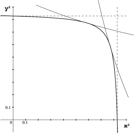
Figure 1: Domain limitations for $x^{2}$ and $y^{2}$.

which is described by the following equation,

$$y^{2}=\frac{B}{A^{2}+BC}=\frac{2(\sqrt{2}-1)-x^{2}}{|(1-\sqrt{2})+\frac{x^{2}}{\sqrt{2}}|^{2}+(2(\sqrt{2}-1)-x^{2})(1+\frac{x^{2}}{2})}$$ (30)

Now the problem of maximizing the probability $p_{j}$ becomes trivial, because $p_{j}=\frac{x^{2}y^{2}}{2}$ and one can simply substitute $y^{2}$ with the value it takes along the curve (30), and maximize $p_{j}$ as a function of only one variable $x^{2}$,

$$p_{j}=\frac{x^{2}}{2}\cdot\frac{2(\sqrt{2}-1)-x^{2}}{|(1-\sqrt{2})+\frac{x^{2}}{\sqrt{2}}|^{2}+(2(\sqrt{2}-1)-x^{2})(1+\frac{x^{2}}{2})}$$ (31)

This takes its maximum value in $x^{2}=y^{2}=\frac{1}{\sqrt{2}}$, which is (see fig. 2), $p_{j}=0.25$.

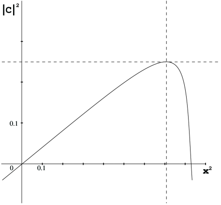
Figure 2: Limitations on success probability of NS-gate: the maximum value is $0.25$.

2.3 Generalizing the Input State

When adding $k$ ancillary modes to the system, we are considering a much more general situation than that described by input $\sigma_{i}$: actually, we are considering the simplest case in which the ancillary Hilbert space is enlarged to an arbitrary dimensionality $k$. This is because the state $|\mathbf{i}\rangle_{A}$ can be transformed in reversible deterministic way to any normalized one-photon state, $|\chi\rangle_{A}=\sum_{i=2}^{k+1}\gamma_{i}a^{{\dagger}}_{i}|0\ldots 0\rangle_{A}$, by a LOP acting only on the $k$ ancillary modes, that we denote by $V=\mathbb{I}_{S}\otimes V_{A}$. Therefore, any circuit acting on $|\psi\rangle_{S}\otimes|\chi\rangle_{A}$ as $U$ can be reduced to one acting on $|\psi\rangle_{S}\otimes|\mathbf{i}\rangle_{A}$ denoted by $U^{{}^{\prime}}=UV$,

$$U(|\psi\rangle_{S}\otimes|\chi\rangle_{A})=U(V(|\psi\rangle_{S}\otimes|\mathbf{i}))=U^{{}^{\prime}}(|\psi\rangle_{S}\otimes|\mathbf{i}\rangle_{A})$$ (32)

and the result of the previous section is still valid with general one-photon input state.

2.4 Generalizing Post-Selection Condition

Further generalization is obtained considering the possibility of implementing the following transformation,

$$|\psi\rangle_{S}\otimes|\mathbf{i}\rangle_{A}\longrightarrow|\psi^{{}^{\prime}}\rangle_{S}\otimes\sum_{j=2}^{s+1}\gamma_{j}a^{{\dagger}}_{j}|0\ldots 0\rangle_{A}$$ (33)

Notice that here the ancillary state is not normalized, due to non-unit probability of success. Even if in this case amplitudes $\gamma_{j}$ cannot be summed, every time the photon is observed in the $j$-th output mode the desired NS-gate transform is obtained, and this happens with probability $p_{j}=|\gamma_{j}|^{2}$.

We are in the situation of a rank-$s$ post-selection condition,

$$P_{s}=\mathbb{I}_{S}\otimes\sum_{j=2}^{s+1}|\mathbf{j}\rangle_{A}\langle\mathbf{j}|$$ (34)

corresponding to the observation of only one photon in whichever of the output modes. Then the total probability of success is, $p_{\textrm{\small{tot}}}=\sum_{j}p_{j}$.

As the simplest example, one could consider the case where $\sigma=|10\rangle_{A}\langle 10|$ and $P=\mathbb{I}_{S}\otimes(|10\rangle_{A}\langle 10|+|01\rangle_{A}\langle 01|)$, and find the following equations for the gate functioning,

$$\underline{U}_{11} = 1-\sqrt{2}$$

$$\underline{U}_{22} = \frac{\underline{U}_{12}\underline{U}_{21}}{1-\underline{U}_{11}}$$

$$\underline{U}_{32} = \frac{\underline{U}_{12}\underline{U}_{31}}{1-\underline{U}_{11}}$$ (35)

so that

$$p_{\textrm{\small{tot}}}=\frac{|\underline{U}_{12}|^{2}}{2}(|\underline{U}_{21}|^{2}|\underline{U}_{31}|^{2})$$ (36)

In general, one has $k=s+m$ ancillary modes, being the photon injected in mode $i\leq s$. The additional $m$ modes are needed to guarantee that the circuit can be implemented as a LOP, namely to make the $\underline{U}$ matrix indeed unitary.

Functioning conditions constrain $\underline{U}$ to be in the form:

$$\left(\begin{array}[]{cccc}1-\sqrt{2}&\ldots&\underline{U}_{1,i}&\ldots\\ \underline{U}_{2,1}&\ldots&\frac{\underline{U}_{2,1}\underline{U}_{1,i}}{\sqrt{2}}&\ldots\\ \vdots&{}\hfil&\vdots&{}\hfil\\ \underline{U}_{s+1,1}&\ldots&\frac{\underline{U}_{s+1,1}U_{1,i}}{\sqrt{2}}&\ldots\\ \underline{U}_{s+2,1}&\ldots&\underline{U}_{s+2,i}&\ldots\\ \vdots&{}\hfil&\vdots&\ddots\end{array}\right)$$ (37)

In this case, the success probability of NS-gate has the following form:

$$p_{\textrm{\small{tot}}}=\frac{|\underline{U}_{1i}|^{2}}{2}\sum_{j=2}^{s+1}|\underline{U}_{j1}|^{2}$$ (38)

Following the lines of the subsection 2.2 one finds that all the calculations are still valid in this case, and $p_{\textrm{\small{tot}}}$ has to be maximized along the curve in fig. 2 with the replacement $x^{2}=\sum_{j=2}^{s+1}|\underline{U}_{j1}|^{2}$. The result is that the same upper bound holds, namely $p_{\textrm{\small{tot}}}\leq 0.25$.

One could have also argued this result, by observing that the global LOP transformation in this case gives:

$$U(|\psi\rangle_{S}\otimes|\mathbf{i}\rangle_{A}) \!\!\!\!=\!\!\!\! |\psi_{+}\rangle_{S}\otimes\gamma_{0}|0\ldots 0\rangle_{A}+|\psi^{{}^{\prime}}\rangle_{S}\otimes\sum_{l=1}^{s+1}\gamma_{l}a^{{\dagger}}_{l}|0\ldots 0\rangle_{A}+$$ (39)

$$\!\!\!\!\!\!\!\!\!\!\!\!\!\!\!\!\!\!\!\!\!\!\!\!\!\!\!\!\!\!\!\!\!\!\!\!\!\!\!\!\!\!\!\!\!\!\!\!\!\!\!\!\!\!\!\!\!\!\!\!\!\!\!\!\!\!\!\!\!\!\!\!\!\!\!\!\!\!\!\!\!\!\!\!\!\!\!\!\!\!\!\!\!\!\!\!\!\!\!\!+ \!\!\!\!\!\!\!\!\!\!\!\!\!\!\!\!\!\!\!\!\!\!\!\!\!\!\!\!\!\!\!\!\!\!\!\!\!\!\!\!\!\!\!\!\!\!\!\!\!\!|\psi_{-}\rangle_{S}\otimes\sum_{l,m=1}^{s+1}\gamma_{lm}a^{{\dagger}}_{l}a^{{\dagger}}_{m}|0\ldots 0\rangle_{A}+|\psi_{--}\rangle_{S}\otimes\sum_{l,m,n=1}^{s+1}\gamma_{lmn}a^{{\dagger}}_{l}a^{{\dagger}}_{m}a^{{\dagger}}_{n}|0\ldots 0\rangle_{A}$$

where indices $+,-$ denote states of the system S with one photon added or subtracted, and $|\psi_{--}\rangle_{S}=|0\rangle_{S}$ necessarily.

The point here is that a subsequent LOP $V$ acting only on modes from $2$ to $s$ before post-selection measurement would leave invariant the subspaces of the ancillary Fock space with any fixed number of photons. Thus, one can always find a suitable $V$ that maps reversibly and deterministically the state (39) to another one of the form:

$$U(|\psi\rangle_{S}\otimes|\mathbf{i}\rangle_{A}) \!\!\!\!=\!\!\!\! |\psi_{+}\rangle_{S}\otimes\gamma_{0}|0\ldots 0\rangle_{A}+|\psi^{{}^{\prime}}\rangle_{S}\otimes|\mathbf{j}\rangle_{A}+$$ (40)

$$\!\!\!\!\!\!\!\!\!\!\!\!\!\!\!\!\!\!\!\!\!\!\!\!\!\!\!\!\!\!\!\!\!\!\!\!\!\!\!\!\!\!\!\!\!\!\!\!\!\!\!\!\!\!\!\!\!\!\!\!\!\!\!\!\!\!\!\!\!\!\!\!\!\!\!\!\!\!\!\!\!\!\!\!\!\!\!\!\!\!\!\!\!\!\!\!\!\!\!\!+ \!\!\!\!\!\!\!\!\!\!\!\!\!\!\!\!\!\!\!\!\!\!\!\!\!\!\!\!\!\!\!\!\!\!\!\!\!\!\!\!\!\!\!\!\!\!\!\!\!\!|\psi_{-}\rangle_{S}\otimes\sum_{l,m=1}^{s+1}\gamma_{lm}a^{{\dagger}}_{l}a^{{\dagger}}_{m}|0\ldots 0\rangle_{A}+|\psi_{--}\rangle_{S}\otimes\sum_{l,m,n=1}^{s+1}\gamma_{lmn}a^{{\dagger}}_{l}a^{{\dagger}}_{m}a^{{\dagger}}_{n}|0\ldots 0\rangle_{A}$$

Once again, the transformation can be brought in the form analyzed in the subsection $2.2$, that is, $V(U(|\psi\rangle_{S}\otimes|\mathbf{i}))=U^{{}^{\prime\prime}}(|\psi\rangle_{S}\otimes|\mathbf{i}\rangle_{A})$

3 Conclusions

In the present paper, we addressed the issue of the maximum success probability of the post-selected NS-gate. Up to now, this problem has no general solution: that is, no upper bound which is both strict and independent of the ancillary resources. Our strategy was to restrict ancillary resources to only one photon and arbitrary number of vacuum states. This has reduced the problem to a mathematically soluble one, still general enough. In fact, we showed that under these conditions the upper bound is $0.25$, it is strict, and it is independent of the dimension of the Hilbert space spanned by the ancillary states. Furthermore, we have considered generalized post-selection conditions, namely those described by rank-r projectors, with $r>1$, so that the problem has been fully solved for the case of a single ancillary photon.

References

• [1] E. Knill, R. Laflamme, and G. Milburn, Nature (London) 409, 46 (2001).
• [2] T.B. Pittman, B.C. Jacobs, and J.D. Franson, Phys.Rev. A 64, 062311 (2001).
• [3] T.C. Ralph, A.G. White, W.J. Munro, and G.J. Milburn, Phys.Rev. A 65, 012314 (2001).
• [4] T.C. Ralph, Langford, T.B. Bell, and A.G. White, Phys.Rev. A 65, 062324 (2002).
• [5] A.P. Lund, and T.C. Ralph, Phys.Rev. A 66, 032327 (2002).
• [6] J.L. Dodd, T.C. Ralph, and G.J. Milburn, Phys.Rev. A 68, 042328 (2003).
• [7] G.L.. Giorgi, F. de Pasquale, and S. Paganelli, Phys.Rev. A 70, 022319 (2004).
• [8] S. Scheel, K. Nemoto, W.J. Munro, and P.L. Knight, Phys.Rev. A 68 032310 (2003).
• [9] G.G. Lapaire, P. Kok, J.P. Dowling, and J.E. Sipe, Phys.Rev. A 68 042314 (2003).
• [10] J. Clausen, L. Knoll, and D.G. Welsch, Phys.Rev. A 68 043822 (2003).
• [11] E. Knill, Phys.Rev. A 66, 052306 (2002).
• [12] E. Knill, quant-ph/0307015.
• [13] S. Scheel, and N. Lutkenhaus, New J. Phys. 6, 51 (2004).